
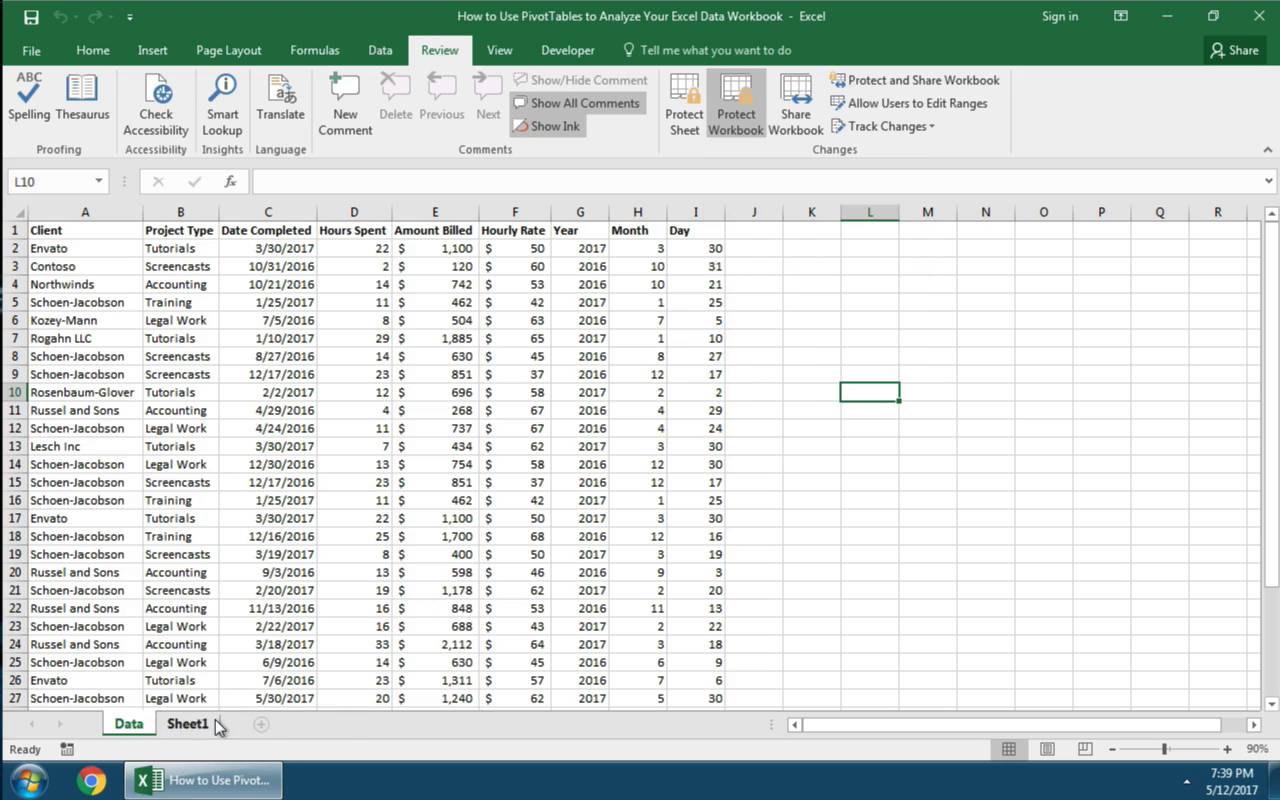
To prevent other users from accidentally or deliberately changing, moving, or deleting data in a worksheet, you can lock the cells on your Excel worksheet and then protect the sheet with a password. Say you own the team status report worksheet, where you want team members to add data in specific cells only and not be able to modify anything else. With worksheet protection, you can make only certain parts of the sheet editable and users will not be able to modify data in any other region in the sheet.
Important: Worksheet level protection is not intended as a security feature. It simply prevents users from modifying locked cells within the worksheet. Protecting a worksheet is not the same as protecting an Excel file or a workbook with a password. See below for more information:
-
To lock your file so that other users can’t open it, see Protect an Excel file.
-
To prevent users from adding, modifying, moving, copying, or hiding/unhiding sheets within a workbook, see Protect a workbook.
-
To know the difference between protecting your Excel file, workbook, or a worksheet see Protection and security in Excel.
The following sections describe how to protect and unprotect a worksheet in Excel for Windows.
Here’s what you can lock in an unprotected sheet:
-
Formulas: If you don’t want other users to see your formulas, you can hide them from being seen in cells or the Formula bar. For more information, see Display or hide formulas.
-
Ranges: You can enable users to work in specific ranges within a protected sheet. For more information, see Lock or unlock specific areas of a protected worksheet.
Note: ActiveX controls, form controls, shapes, charts, SmartArt, Sparklines, Slicers, Timelines, to name a few, are already locked when you add them to a spreadsheet. But the lock will work only when you enable sheet protection. See the subsequent section for more information on how to enable sheet protection.
Worksheet protection is a two-step process: the first step is to unlock cells that others can edit, and then you can protect the worksheet with or without a password.
Step 1: Unlock any cells that needs to be editable
-
In your Excel file, select the worksheet tab that you want to protect.
-
Select the cells that others can edit.
Tip: You can select multiple, non-contiguous cells by pressing Ctrl+Left-Click.
-
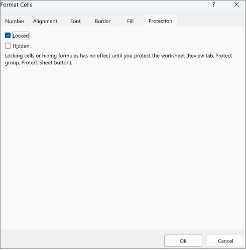
Right-click anywhere in the sheet and select Format Cells (or use Ctrl+1, or Command+1 on the Mac), and then go to the Protection tab and clear Locked.

Step 2: Protect the worksheet
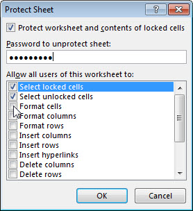
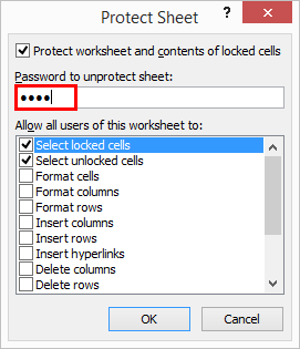
Next, select the actions that users should be allowed to take on the sheet, such as insert or delete columns or rows, edit objects, sort, or use AutoFilter, to name a few. Additionally, you can also specify a password to lock your worksheet. A password prevents other people from removing the worksheet protection—it needs to be entered to unprotect the sheet.
Given below are the steps to protect your sheet.
-
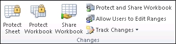
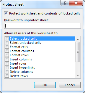
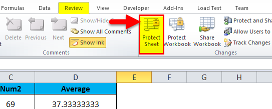
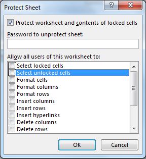
On the Review tab, click Protect Sheet.
-
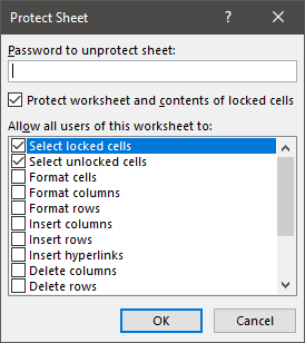
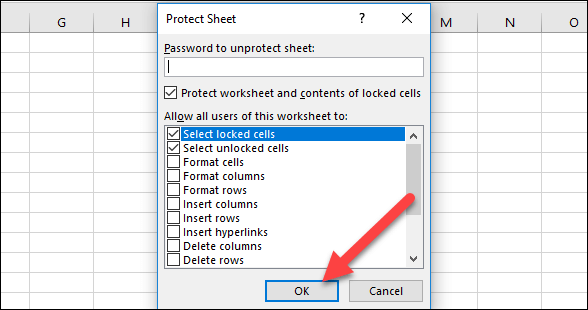
In the Allow all users of this worksheet to list, select the elements you want people to be able to change.
Option
Allows users to
Select locked cells
Move the pointer to cells for which the Locked box is checked on the Protection tab of the Format Cells dialog box. By default, users are allowed to select locked cells.
Select unlocked cells
Move the pointer to cells for which the Locked box is unchecked on the Protection tab of the Format Cells dialog box. By default, users can select unlocked cells, and they can press the TAB key to move between the unlocked cells on a protected worksheet.
Format cells
Change any of the options in the Format Cells or Conditional Formatting dialog boxes. If you applied conditional formatting before you protected the worksheet, the formatting continues to change when a user enters a value that satisfies a different condition.
Format columns
Use any of the column formatting commands, including changing column width or hiding columns (Home tab, Cells group, Format button).
Format rows
Use any of the row formatting commands, including changing row height or hiding rows (Home tab, Cells group, Format button).
Insert columns
Insert columns.
Insert rows
Insert rows.
Insert hyperlinks
Insert new hyperlinks, even in unlocked cells.
Delete columns
Delete columns.
Note: If Delete columns is protected and Insert columns is not protected, a user can insert columns but cannot delete them.
Delete rows
Delete rows.
Note: If Delete rows is protected and Insert rows is not protected, a user can insert rows but cannot delete them.
Sort
Use any commands to sort data (Data tab, Sort & Filter group).
Note: Users can’t sort ranges that contain locked cells on a protected worksheet, regardless of this setting.
Use AutoFilter
Use the drop-down arrows to change the filter on ranges when AutoFilters are applied.
Note: Users cannot apply or remove AutoFilter on a protected worksheet, regardless of this setting.
Use PivotTable reports
Format, change the layout, refresh, or otherwise modify PivotTable reports, or create new reports.
Edit objects
Doing any of the following:
-
Make changes to graphic objects including maps, embedded charts, shapes, text boxes, and controls that you did not unlock before you protected the worksheet. For example, if a worksheet has a button that runs a macro, you can click the button to run the macro, but you cannot delete the button.
-
Make any changes, such as formatting, to an embedded chart. The chart continues to be updated when you change its source data.
-
Add or edit notes.
Edit scenarios
View scenarios that you have hidden, making changes to scenarios that you have prevented changes to, and deleting these scenarios. Users can change the values in the changing cells, if the cells are not protected, and add new scenarios.
-
-
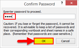
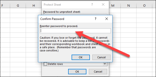
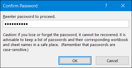
Optionally, enter a password in the Password to unprotect sheet box and click OK. Reenter the password in the Confirm Password dialog box and click OK.
Important:
-
Use strong passwords that combine uppercase and lowercase letters, numbers, and symbols. Weak passwords don’t mix these elements. Passwords should be 8 or more characters in length. A passphrase that uses 14 or more characters is better.
-
It is critical that you remember your password. If you forget your password, Microsoft cannot retrieve it.
-
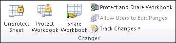
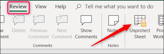
The Protect Sheet option on the ribbon changes to Unprotect Sheet when a sheet is protected. To view this option, click the Review tab on the ribbon, and in Changes, see Unprotect Sheet.
To unprotect a sheet, follow these steps:
-
Go to the worksheet you want to unprotect.
-
Go to File > Info > Protect > Unprotect Sheet, or from the Review tab > Changes > Unprotect Sheet.
-
If the sheet is protected with a password, then enter the password in the Unprotect Sheet dialog box and click OK.
The following sections describe how to protect and unprotect a worksheet in Excel for the Web.
-
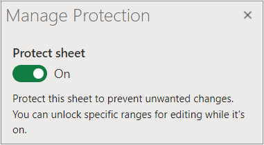
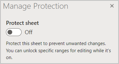
Select Review > Manage Protection.
-
To turn on protection, in the Manage Protection task pane, select Protect sheet.
Note Although you can selectively protect parts of the sheet by setting various options in the Options section, these settings only apply when the Protect sheet setting is on.
-
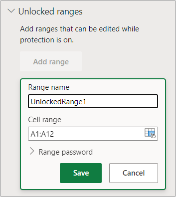
By default, the entire sheet is locked and protected. To unlock specific ranges, select Unlocked ranges, and then enter a range name and cell range. You can add more than one range.
-
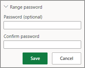
Optionally, to require a password to edit a range, select Range password, enter and confirm the password, and then select Save. Make sure sheet protection is turned on.
-
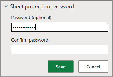
Optionally, to control the ability to edit protections for the entire sheet with a password, select Sheet protection password, enter and confirm the password, and then select Save.
Important-
Use strong passwords that combine uppercase and lowercase letters, numbers, and symbols. Weak passwords don’t mix these elements. Passwords should be 8 or more characters in length. Make sure the CAPS LOCK key is off and use correct capitalization. Passwords are case-sensitive.
-
It is critical that you remember your password. If you forget your password, Microsoft cannot retrieve it.
-
-
Optionally, if you want to selectively enable and disable specific sheet elements, select the Options section, and then select one or more options.
Option
Allows users to
Select locked cells
Move the pointer to cells for which the Locked box is checked on the Protection tab of the Format Cells dialog box. By default, users are allowed to select locked cells.
Select unlocked cells
Move the pointer to cells for which the Locked box is unchecked on the Protection tab of the Format Cells dialog box. By default, users can select unlocked cells, and they can press the TAB key to move between the unlocked cells on a protected worksheet.
Format cells
Change any of the options in the Font and Alignment groups of the Home tab.
Note If cell formatting and hidden properties were previously protected by using the Format Cells or Conditional Formatting dialog boxes, they remain protected, but you can only modify options in these dialog boxes by using Excel for Windows. If you applied conditional formatting before you protected the worksheet, the formatting continues to change when a user enters a value that satisfies a different condition.
Format columns
Use any of the column formatting commands, including changing column width or hiding columns (Home tab, Cells group, Format button).
Format rows
Use any of the row formatting commands, including changing row height or hiding rows (Home tab, Cells group, Format button).
Insert columns
Insert columns.
Insert rows
Insert rows.
Insert hyperlinks
Insert new hyperlinks, even in unlocked cells.
Delete columns
Delete columns.
Note: If Delete columns is protected and Insert columns is not protected, a user can insert columns but cannot delete them.
Delete rows
Delete rows.
Note: If Delete rows is protected and Insert rows is not protected, a user can insert rows but cannot delete them.
Sort
Use any commands to sort data (Data tab, Sort & Filter group).
Note: Users can’t sort ranges that contain locked cells on a protected worksheet, regardless of this setting.
Use AutoFilter
Use the drop-down arrows to change the filter on ranges when AutoFilters are applied.
Note: Users cannot apply or remove AutoFilter on a protected worksheet, regardless of this setting.
Use PivotTable reports
Format, change the layout, refresh, or otherwise modify PivotTable reports, or create new reports.
Edit objects
Doing any of the following:
-
Make changes to graphic objects including maps, embedded charts, shapes, text boxes, and controls that you did not unlock before you protected the worksheet. For example, if a worksheet has a button that runs a macro, you can click the button to run the macro, but you cannot delete the button.
-
Make any changes, such as formatting, to an embedded chart. The chart continues to be updated when you change its source data.
-
Add or edit notes.
Edit scenarios
View scenarios that you have hidden, making changes to scenarios that you have prevented changes to, and deleting these scenarios. Users can change the values in the changing cells, if the cells are not protected, and add new scenarios.
Notes
-
If you don’t want other users to see your formulas, you can hide them from being seen in cells or the Formula bar. For more information, see Display or hide formulas.
-
ActiveX controls, form controls, shapes, charts, SmartArt, Sparklines, Slicers, Timelines, and so on, are already locked when you add them to a spreadsheet. But the lock works only when you enable sheet protection. For more information, see Protect controls and linked cells on a worksheet.
-
There are two ways to unprotect a sheet, disable it or pause it.
Disable protection
-
Select Review > Manage Protection.
-
To turn off protection, In the Manage Protection task pane, turn off Protect sheet.
Pause protection
Pausing protection turns off protection for the current editing session while maintaining the protection for other users in the workbook. For example, you can pause protection to edit a locked range but maintain protection for other users.
-
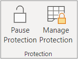
To pause sheet protection, select Review > Pause Protection.
Note If the sheet has a protection password, you must enter that password to pause protection.
-
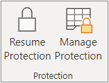
To resume sheet protection, select Review > Resume Protection.
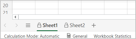
At the bottom of the sheet, the sheet tab displays a locked icon if the sheet is protected (Sheet1), and an unlocked icon if it is paused (Sheet2).
See Also
Protection and security in Excel
Protect an Excel file
Protect a workbook
Lock or unlock specific areas of a protected worksheet
Lock cells to protect them
Display or hide formulas
Protect controls and linked cells on a worksheet
Copy and paste in a protected worksheet
Video: Password protect workbooks and worksheets (Excel 2013)
When it comes time to send your Excel spreadsheet, it’s important to protect the data that you’re sharing. You might want to share your data, but that doesn’t mean it should be changed by someone else.
Spreadsheets often contain essential data that shouldn’t be modified or removed by the recipient. Luckily, Excel has built-in features to protect your spreadsheets.
In this tutorial, I’ll help you make sure that your Excel workbooks maintain data integrity. Here are three key techniques you’ll learn in this tutorial:
- Password protect entire workbooks to prevent them from being opened by unauthorized users.
- Protect individual sheets and the workbook structure, to prevent the insertion or deletion of sheets in the workbook.
- Protect cells, to specifically allow or disallow changes to key cells or formulas in your Excel spreadsheets.
Even users with the best intentions may accidentally break an important or complex formula. The best thing to do is remove the option to change your spreadsheets altogether.
How to Protect Excel: Cells, Sheets, & Workbooks (Watch & Learn)
In the screencast below, you’ll see me work through several important types of protection in Excel. We’ll protect an entire workbook, a single spreadsheet, and more.
Want a step-by-step walkthrough? Check out my steps below to find out how to use these techniques. You’ll learn how to protect your workbook in Excel, as well as protecting individual worksheets, cells, and how to work with advanced settings.
We start with broader worksheet protections, then work down to narrower targeted protections you can apply in Excel. Let’s get started learning how to protect your spreadsheet data:
1. Password Protect an Excel Workbook File
Let’s start off by protecting an entire Excel file (or workbook) with a password to prevent others from opening it.
This is a breeze to do. While working in Excel, navigate to the File tab choose the Info tab. Click on the Protect Workbook dropdown option and choose Encrypt with Password.
As is the case with any password, choose a strong and secure combination of letters, numbers, and characters, bearing in mind that passwords are case-sensitive.


It’s important to note that Microsoft has really beefed up the seriousness of their password protection in Excel. In prior versions, there were easy workarounds to bypass password protection of Excel workbooks, but not in newer versions.


In Excel 2013 and beyond, the password implementation will prevent these traditional methods to bypass it. Make sure that you store your passwords carefully and safely or you risk permanently losing access to your crucial workbooks.
Excel Workbook — Mark as Final
If you want to be a bit less forceful with your spreadsheets, consider using the Mark as Final feature. When you mark an Excel file as the final version, it switches the file to read-only mode, and the user will have to re-enable editing.
To change a file to read-only mode, return to the File > Info button, and click on Protect Workbook again. Click on Mark as Final and confirm that you want to mark the document as a final version.


Marking a file as the final version will add a soft warning to the top of the file. Anyone who opens the file after it has been marked as final will see a notice, warning them that the file is finalized.


Marking a file as the final version is a less formal way of signaling that a file shouldn’t be changed further. The recipient still has the ability to click Edit Anyway and modify the spreadsheet. Marking a file as the final edition is more like a suggestion, but it’s a great approach if you trust the other file users.
2. Password Protect Your Excel Sheet Structure
Next up, let’s learn how to protect the structure of an Excel workbook. This option will ensure that no sheets are deleted, added, or re-arranged inside of the workbook.
If you want everyone to be able to access the workbook, but limit the changes they can make to a file, this is a great start. This protects the structure of the workbook, and limits how the user can change the sheets inside of it.
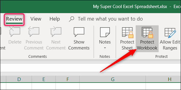
To turn on this protection, go to the Review tab on Excel’s ribbon and click on Protect Workbook.


Once this option is turned on, the following will go into effect:
- No new sheets can be added to the workbook.
- No sheets can be deleted from the workbook.
- Sheets can no longer be hidden or unhidden from the user’s view.
- The user can no longer drag and drop the sheet tabs to reorder them in the workbook.
Of course, trusted users can be given the password to unprotect the workbook and modify it. To unprotect a workbook, simply click on the Protect Workbook button again and input the password to unprotect the Excel workbook.


3. How to Protect Cells in Excel
Now, let’s get down to really detailed methods for protecting a spreadsheet. So far, we’ve been password protecting an entire workbook or the structure of an Excel file. In this section, we dig into how to protect your cells in Excel with specific settings you can apply. We cover how to allow or block certain types of changes to be made to parts of your spreadsheet.
To get started, find Excel’s Review tab, and click on Protect Sheet. On the pop-up window, you’ll see a huge set of options. This window allows you to fine-tune how you want to protect the cells in your Excel spreadsheet. For now, let’s leave the settings at their default.


This option allows for very specific protections of your spreadsheet. By default, the options will almost totally lock down the spreadsheet. Let’s add a password so that the sheet is protected. If you press OK at this point, let’s see what happens when you attempt to change a cell.


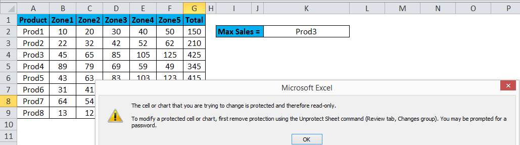
Excel throws off an error that the cell is protected, which is exactly what we wanted.
Basically, this option is crucial if you want to ensure that your spreadsheet isn’t changed by others who have access to the file. Using the protect sheet feature is a way that you can selectively protect the spreadsheet.
To unprotect the sheet, simply click on the Protect Sheet button and re-enter the password to remove the protections added to the sheet.
Specific Protections in Excel
Let’s take a second look at the options that show when you start to protect a sheet in Excel workbooks.

The Protect Sheet menu lets you refine the options for sheet protection. Each of the boxes on this menu lets the user change slightly more inside of a protected worksheet.
To remove a protection, check the respective box in the list. For example, you could allow the spreadsheet user to Format cells by checking the corresponding box.
Here are two ideas on how you could selectively allow the user to change the spreadsheet:
- Check the Format cells, columns, and rows boxes to let the user change the visual appearance of cells without modifying the original data.
- Insert columns and rows could be checked so that the user can add more data, while protecting the original cells.
The important box to leave checked is the Protect worksheet and contents of locked cells box. This protects the data inside of cells.
When you’re working with crucial financial data or formulas that will be used in making decisions, you have to maintain control of the data and ensure that it doesn’t change. Using these types of targeted protections is an important Excel skill to master.
Recap and Keep Learning More About Excel
Locking up a spreadsheet before you send it is crucial to protecting your valuable data and making sure that it’s not misused. The tips I shared in this tutorial help you maintain control of that data even after your Excel spreadsheet is forwarded and shared.
All of these tips are additional tools and steps to becoming an advanced Excel user. Protecting your workbooks is a specific skill, but there are lots of ways to improve your performance. As always, there’s room to grow your Excel skills further. Here are some helpful Excel tutorials with important skills to master next:
- PivotTables are a great tool for working with spreadsheet data. Here’s 5 Advanced Excel Pivot Table Techniques to learn now.
- ExcelZoo has a listing of additional tutorials for protecting your workbooks, sheets, and cells.
- Condition formatting changes how a cell looks based on what’s inside of it. Here’s a comprehensive Excel tutorial on How to Use Conditional Formatting.
How do you protect your important business data when sharing it? Let me know in the comments section if you use these protection tools or others I may not know about.
Did you find this post useful?

I believe that life is too short to do just one thing. In college, I studied Accounting and Finance but continue to scratch my creative itch with my work for Envato Tuts+ and other clients. By day, I enjoy my career in corporate finance, using data and analysis to make decisions.
I cover a variety of topics for Tuts+, including photo editing software like Adobe Lightroom, PowerPoint, Keynote, and more. What I enjoy most is teaching people to use software to solve everyday problems, excel in their career, and complete work efficiently. Feel free to reach out to me on my website.
Protecting Excel Sheet
Protect worksheet is a feature in Excel when we do not want any other user to make changes to our worksheet. It is available in the “Review” tab of Excel. It has various features where we can allow users to perform some tasks but not make changes, such as they can select cells to use an AutoFilter but cannot make any changes to the structure. Also, it is recommended to protect a worksheet with a password.
An Excel worksheet that is protected using a password and/or has the cells in the worksheet locked to prevent any changes is known as a “Protect Sheet.”
Purpose of a Protecting sheet with a password
To prevent the unknown users from accidentally or purposely changing, editing, moving, or deleting data in a worksheet, you can lock the cells in the Excel worksheet and then protect an Excel sheet with a password.
Table of contents
- Protecting Excel Sheet
- #1 How to Protect a Sheet in Excel?
- #2 How to Protect Cells in an Excel Worksheet?
- #3 How to Hide the Formula Associated with a Cell?
- Pros
- Cons
- Things to Remember
- Recommended Articles
#1 How to Protect a Sheet in Excel?
Below are the steps for protecting the sheet in Excel:
- First, open the worksheet you wish to save. Then, right-click the worksheet or go to “Review” and “Protect Sheet.” The option lies in the “Changes” group, then click on “Protect Sheet” from the list of options displayed.

- It will prompt you to enter a password.

- Insert the password as per choice.
- The section below displays a list of options you can allow the users of the worksheet to perform. Every action has a checkbox. Check those actions you wish to enable the worksheet users to complete.
- If no action is checked, the users may only VIEW the file and not perform any updates by default. Click on “OK.”
- Re-enter the password as prompted on the second screen. Then, click on “OK.”


#2 How to Protect Cells in an Excel Worksheet?
To protect cells in Excel, follow the steps given below:
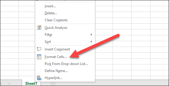
- Step 1: Right, click on the Excel cell you wish to protect. Then, select “Format Cells” from the menu displayed.
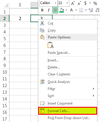
- Step 2: Go to the tab named “Protection.”

- Step 3: Check “Locked” if you wish to lock the cell in Excel. It will prevent the cell from editing, and we can only view the content. Check “Hidden” if you wish to hide the cell. It will hide the cell and so the content.

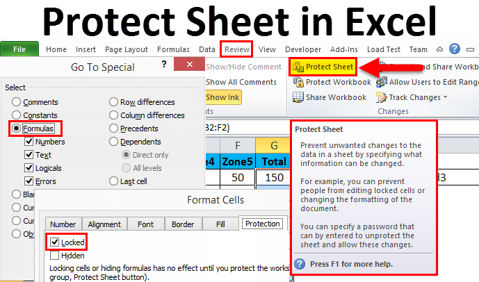
#3 How to Hide the Formula Associated with a Cell?
- Step 1: As shown below, cell F2 has a formula: D2+E2 = F2.

- Step 2: Below shows that the Excel cell is protected as “Locked” and “Hidden” as both the options are checked.

- Step 3: As a result, the formula is hidden / not visible in the formula bar, as shown below.

- Step 4: Upon unprotecting the sheet, the formula also starts appearing in the formula bar, as shown below.

Pros
- A protected Excel sheet with a password is used to secure sensitive information from unwanted changes done by unauthorized entities.
- Excel worksheet cell actions are access controlled. It means they can be configured to be available for some users and not others.
Cons
- If you protect an Excel sheet with a password, and if it is forgotten, it is non-recoverable. It means there is no automated or manual way of resetting or recovering the old password. It can cause data loss.
Things to Remember
- The password of the protected sheet is case-sensitive.
- The password of the protected sheet is non-recoverable.
- If no actions are checked in the “Protect Sheet” dialog window, the default accessibility is “View.” It means the others can view the protected worksheet and cannot add new data or make any changes to the cells in the worksheet.
- Protecting the sheet is mandatory if one wishes to protect the cells as locked or hidden.
- If the sheet is unprotected in ExcelOnce the workbook has been password-protected, one must input the exact password that was entered while protecting the workbook in order to unprotect it.read more, all the formatting/locking associated with the cells would be overridden/gone.
- Locking a cell in Excel prevents it from making any changes.
- Hiding a cell hides the formula associated with it, making it invisible in the formula bar.
Recommended Articles
This article is a guide to Protect Sheet in Excel. We discuss how to protect sheets in Excel, practical examples, and downloadable Excel templates. You may learn more about Excel from the following articles: –
- VBA UnProtect Sheet
- Vba Protect SheetVBA Protect Sheet is an In-built function that protects the worksheet with a password & prohibits the users from editing, deleting, or moving the contained data. read more
- Scroll Lock in ExcelWhen we press the down arrow key from any cell, it normally moves us to the next cell below it, but when we have scroll lock turned on, it drags the worksheet down while the cursor stays in the same cell.read more
- Lock Cells in ExcelIn Excel, cells are locked to protect them from unwanted editing, deleting, and overwriting. Locking cells is specifically beneficial in cases where an excel worksheet needs to be shared with several colleagues.read more
- Split Panes in ExcelSplitting panes in excel means splitting a workbook in different parts, this technique is available in the windows section of the View tab, panes can be split in horizontal or vertical way or it can be a cross split, the horizontal and vertical split can be seen in the mid-section of the worksheet however cross split can be done by dragging the panes.read more
Reader Interactions
Excel Protect Sheet (Table of Contents)
- Introduction to Protect Sheet
- How to Protect (Lock) Cells in Excel?
Introduction to Protect Sheet in Excel
Protect Sheet in Excel is used to protect and safeguard the data in any workbook and worksheet with the help of setting up a password in it. There are 2 ways to protect the sheet. One is by selecting the Protect Sheet option from the right-click menu list on Sheet’s name, and the other is choosing the Protect Sheet option, which is in the Review menu option under the Changes section. Once we click on it, we will get a protect sheet box that has all the possible options to lock the sheet. We can lock any row, column, cells by sorting. Choose an option as we choose and then enter the password to protect the sheet. And there is no limit to password characters.
How to Protect (Lock) Cells in Excel?
It is very simple and easy to protect cells in Excel. Let’s understand the working of protecting cells in excel with some examples.
You can download this Print Gridlines Excel Template here – Print Gridlines Excel Template
Example #1
Suppose we have an Excel with three different values. Our objective is to calculate their average.
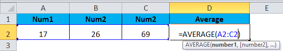
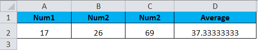
As we can see from the screenshot above, we have three values in cell A2, B2, and C2. We calculate the average of these numbers in cell D2. Now we wish to lock the cell D2, which contains the formula, so that it doesn’t get accidentally altered when the excel is passed from one person to another.
Now, since all cells are locked in Excel by default, let us first unlock them. To do this, we first need to select all the cells by pressing Ctrl+A or Command+A. Next, open the Format Cells dialog box by pressing Ctrl+1.
Now we will need to go to the “Protection” tab.

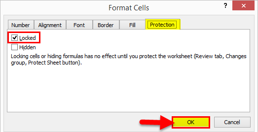
Now under the “Protection” tab, we will need to untick the “Locked” option and click OK. All the cells in the worksheet will then be unlocked.
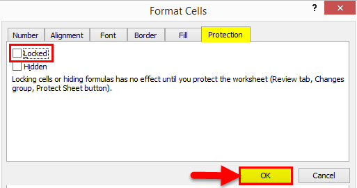
Now, we will need to select the cell that contains the formula, i.e. cell D2. We will now press Ctrl+1. This will once again open the Format Cells dialog box. We will navigate to the Protection tab.

This will lock the cell formula. Now, we have to protect the formula. To do this, we will need to navigate to the “Review” tab and click on the “Protect Sheet” option.

This will open up the next dialog box, as shown below.
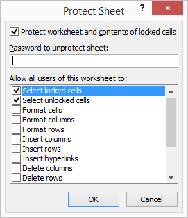
It is also possible to provide a password to protect the sheet. This will result in Excel asking for a password when a user tries to access this Excel sheet.

At this point, Excel will prompt to ask you to re-enter your password just to make sure that there are no mistakes with the password.
After this, the cell will be locked, and it will no longer allow any further modifications to be made. If we click on this cell and try to press any keys in order to modify the formula, we will get the following pop up message.
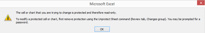
It is interesting to note that only this particular cell is protected, and no other cell will result in a similar pop up upon modification. A locked cell does not guarantee that the underlying formula will be protected from modifications. Therefore, it is vital to protect the formula after locking the cell. Thus, we will need to unlock all the cells first and then lock the formula cell and then protect the formula. This will prevent the formula cell from any accidental modifications, while all the other cells are open to modifications.
Example #2
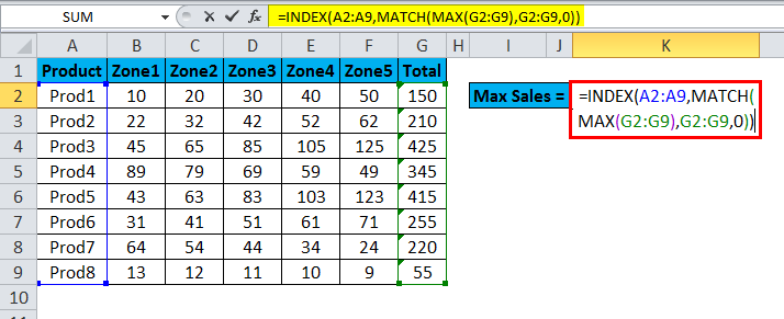
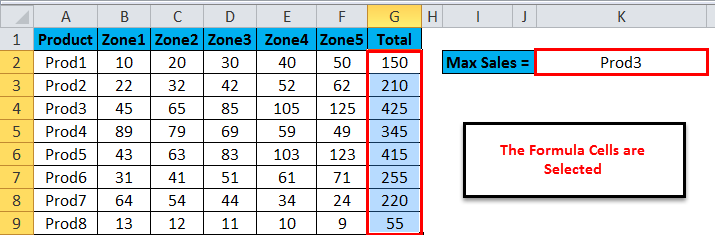
Now, let us suppose that we have sales data for several products in different zones. Our objective is to calculate the total sales for each product separately and then identify the product with the highest sales. We need to lock the cell with the formula to calculate the highest sales and protect it from modifications. However, the cells with the summation formula and the sales data itself should be modifiable.
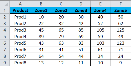
We will first calculate the total sales for each product.
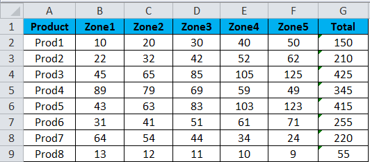
So, to do this, we applied the SUM () function, passed the array for the first row, and then dragged the formula to the remaining rows since the column range for summation for all rows is the same.
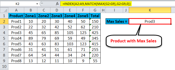
Next, we will find the max sales. Adjacent to this table, we will select a cell and key in the index-match formula to find the product with the max sales.
Now, we need to lock and protect the cell with the formula for Max Sales. Since all cells are locked in Excel by default, let us first unlock them. To do this, we first need to select all the cells by pressing Ctrl+A or Command+A. Next, open the Format Cells dialog box by pressing Ctrl+1.
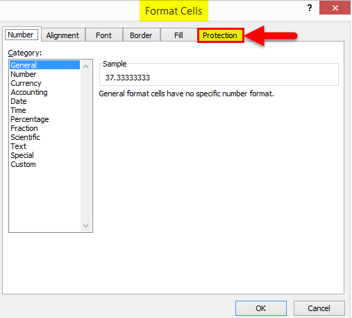
Now we will need to go to the “Protection” tab.
Now under the “Protection” tab, we will need to untick the “Locked” option and click OK. All the cells in the worksheet will then be unlocked.

Now, we will need to select the cell that contains the formula, i.e. cell D2. We will now press Ctrl+1. This will once again open the Format Cells dialog box. We will navigate to the Protection tab.
This will lock the cell formula. Now, we have to protect the formula. To do this, we will need to navigate to the “Review” tab and click on the “Protect Sheet” option.
This will open up the next dialog box, as shown below.

It is also possible to provide a password to protect the sheet. This will result in Excel asking for a password when a user tries to access this Excel sheet.
At this point, Excel will prompt to ask you to re-enter your password just to make sure that there are no mistakes with the password.

After this, the cell will be locked, and it will no longer allow any further modifications. If we click on this cell and try to press any keys in order to modify the formula, we will get the following pop up message.
Alternatively, after unlocking all cells in the worksheet, we can go to the “Home” tab and then navigate to the “Editing” section and select “Find & Select”, and from the dropdown, we can select “Go To Special”.
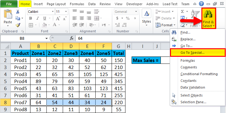
- Excel would then open up the “Go To Special” dialog box, and we would then need to select “Formula” and click on OK. This would then select all the cells which have the formula in their contents.
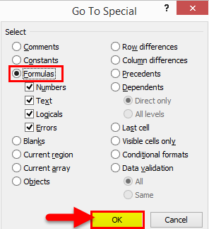
- We can now repeat the process of locking the formula cells and then protecting the formula.
Things to Remember About Protect Sheet in Excel
- Simply locking the cells in Excel does not guarantee protection from accidental modifications.
- We will need to both locks the cells and protect the formulae to completely make them tamper-proof.
- By default, all cells in the workbook are locked.
- Like the first point, simply protecting the formula cells without locking them first would not guarantee accidental modifications.
Recommended Articles
This has been a guide to Protect Sheet in Excel. Here we discuss how to Protect the Sheet in Excel along with practical examples and a downloadable excel template. You can also go through our other suggested articles-
- VBA Protect Sheet
- Unprotect Excel Workbook
- Excel Unprotect Sheet
- Worksheets in Excel
Protecting and unprotecting sheets is a common action for an Excel user. There is nothing worse than when somebody, who doesn’t know what they’re doing, overtypes essential formulas and cell values. It’s even worse when that person happens to be us; all it takes is one accidental keypress, and suddenly the entire worksheet is filled with errors. In this post, we explore using VBA to protect and unprotect sheets.
Protection is not foolproof but prevents accidental alteration by an unknowing user.
Sheet protection is particularly frustrating as it has to be applied one sheet at a time. If we only need to protect a single sheet, that’s fine. But if we have more than 5 sheets, it is going to take a while. This is why so many people turn to a VBA solution.
The VBA Code Snippets below show how to do most activities related to protecting and unprotecting sheets.
Download the example file: Click the link below to download the example file used for this post:
Adapting the code for your purposes
Unless stated otherwise, every example below is based on one specific worksheet. Each code includes Sheets(“Sheet1”)., this means the action will be applied to that specific sheet. For example, the following protects Sheet1.
Sheets("Sheet1").ProtectBut there are lots of ways to reference sheets for protecting or unprotecting. Therefore we can change the syntax to use one of the methods shown below.
Using the active sheet
The active sheet is whichever sheet is currently being used within the Excel window.
ActiveSheet.ProtectApplying a sheet to a variable
If we want to apply protection to a sheet stored as a variable, we could use the following.
Dim ws As Worksheet

Set ws = Sheets("Sheet1")

ws.Protect
Later in the post, we look at code examples to loop through each sheet and apply protection quickly.
Let’s begin with some simple examples to protect and unprotect sheets in Excel.
Protect a sheet without a password
Sub ProtectSheet()

'Protect a worksheet
Sheets("Sheet1").Protect

End Sub
Unprotect a sheet (no password)
Sub UnProtectSheet()

'Unprotect a worksheet
Sheets("Sheet1").Unprotect

End Sub
Protecting and unprotecting with a password
Adding a password to give an extra layer of protection is easy enough with VBA. The password in these examples is hardcoded into the macro; this may not be the best for your scenario. It may be better to apply using a string variable, or capturing user passwords with an InputBox.
VBA Protect sheet with password
Sub ProtectSheetWithPassword()

'Protect worksheet with a password
Sheets("Sheet1").Protect Password:="myPassword"

End Sub
VBA Unprotect sheet with a password
Sub UnProtectSheetWithPassword()

'Unprotect a worksheet with a password
Sheets("Sheet1").Unprotect Password:="myPassword"

End Sub
NOTE – It is not necessary to unprotect, then re-protect a sheet to change the settings. Instead, just protect again with the new settings.
Using a password based on user input
Using a password that is included in the code may partly defeat the benefit of having a password. Therefore, the codes in this section provide examples of using VBA to protect and unprotect based on user input. In both scenarios, clicking Cancel is equivalent to entering no password.
Protect with a user-input password
Sub ProtectSheetWithPasswordFromUser()

'Protect worksheet with a password
Sheets("Sheet1").Protect Password:=InputBox("Enter a protection password:")

End Sub
Unprotect with a user-input password
Sub UnProtectSheetWithPasswordFromUser()

'Protect worksheet with a password
Sheets("Sheet1").Unprotect _
    Password:=InputBox("Enter a protection password:")

End Sub
Catching errors when incorrect password entered
If an incorrect password is provided, the following error message displays.
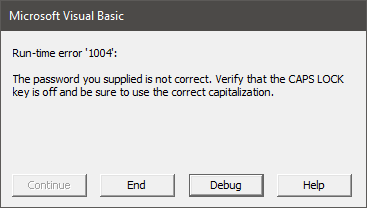
The code below catches the error and provides a custom message.
Sub CatchErrorForWrongPassword()

'Keep going even if error found
On Error Resume Next

'Apply the wrong password
Sheets("Sheet1").Unprotect Password:="incorrectPassword"

'Check if an error has occured
If Err.Number <> 0 Then
    MsgBox "The Password Provided is incorrect"
    Exit Sub
End If

'Reset to show normal error messages
On Error GoTo 0

End Sub
If you forget a password, don’t worry, the protection is easy to remove.
Applying protection to different parts of the worksheet
VBA provides the ability to protect 3 aspects of the worksheet:
- Contents – what you see on the grid
- Objects – the shapes and charts which are on the face of the grid
- Scenarios – the scenarios contained in the What If Analysis section of the Ribbon
By default, the standard protect feature will apply all three types of protection at the same time. However, we can be specific about which elements of the worksheet are protected.
Protect contents
Sub ProtectSheetContents()

'Apply worksheet contents protection only
Sheets("Sheet1").Protect Password:="myPassword", _
    DrawingObjects:=False, _
    Contents:=True, _
    Scenarios:=False

End Sub
Protect objects
Sub ProtectSheetObjects()

'Apply worksheet objects protection only
Sheets("Sheet1").Protect Password:="myPassword", _
    DrawingObjects:=True, _
    Contents:=False, _
    Scenarios:=False

End Sub
Protect scenarios
Sub ProtectSheetScenarios()

'Apply worksheet scenario protection only
Sheets("Sheet1").Protect Password:="myPassword", _
    DrawingObjects:=False, _
    Contents:=False, _
    Scenarios:=True

End Sub
Protect contents, objects and scenarios
Sub ProtectSheetAll()

'Apply worksheet protection to contents, objects and scenarios
Sheets("Sheet1").Protect Password:="myPassword", _
    DrawingObjects:=True, _
    Contents:=True, _
    Scenarios:=True

End Sub
Applying protection to multiple sheets
As we have seen, protection is applied one sheet at a time. Therefore, looping is an excellent way to apply settings to a lot of sheets quickly. The examples in this section don’t just apply to Sheet1, as the previous examples have, but include all worksheets or all selected worksheets.
Protect all worksheets in the active workbook
Sub ProtectAllWorksheets()

'Create a variable to hold worksheets
Dim ws As Worksheet

'Loop through each worksheet in the active workbook
For Each ws In ActiveWorkbook.Worksheets

    'Protect each worksheet
    ws.Protect Password:="myPassword"

Next ws

End Sub
Protect the selected sheets in the active workbook
Sub ProtectSelectedWorksheets()

Dim ws As Worksheet
Dim sheetArray As Variant

'Capture the selected sheets
Set sheetArray = ActiveWindow.SelectedSheets

'Loop through each worksheet in the active workbook
For Each ws In sheetArray

    On Error Resume Next

    'Select the worksheet
    ws.Select

    'Protect each worksheet
    ws.Protect Password:="myPassword"

    On Error GoTo 0

Next ws

sheetArray.Select

End Sub
Unprotect all sheets in active workbook
Sub UnprotectAllWorksheets()

'Create a variable to hold worksheets
Dim ws As Worksheet

'Loop through each worksheet in the active workbook
For Each ws In ActiveWorkbook.Worksheets

'Unprotect each worksheet
ws.Unprotect Password:="myPassword"

Next ws

End Sub
Checking if a worksheet is protected
The codes in this section check if each type of protection has been applied.
Check if Sheet contents is protected
Sub CheckIfSheetContentsProtected()

'Check if worksheets contents is protected
If Sheets("Sheet1").ProtectContents Then MsgBox "Protected Contents"

End Sub
Check if Sheet objects are protected
Sub CheckIfSheetObjectsProtected()

'Check if worksheet objects are protected
If Sheets("Sheet1").ProtectDrawingObjects Then MsgBox "Protected Objects"

End Sub
Check if Sheet scenarios are protected
Sub CheckIfSheetScenariosProtected()

'Check if worksheet scenarios are protected
If Sheets("Sheet1").ProtectScenarios Then MsgBox "Protected Scenarios"

End Sub
Changing the locked or unlocked status of cells, objects and scenarios
When a sheet is protected, unlocked items can still be edited. The following codes demonstrate how to lock and unlock ranges, cells, charts, shapes and scenarios.
When the sheet is unprotected, the lock setting has no impact. Each object becomes locked on protection.
All the examples in this section set each object/item to lock when protected. To set as unlocked, change the value to False.
Lock a cell
Sub LockACell()

'Changing the options to lock or unlock cells
Sheets("Sheet1").Range("A1").Locked = True

End Sub
Lock all cells
Sub LockAllCells()

'Changing the options to lock or unlock cells all cells
Sheets("Sheet1").Cells.Locked = True

End Sub
Lock a chart
Sub LockAChart()

'Changing the options to lock or unlock charts
Sheets("Sheet1").ChartObjects("Chart 1").Locked = True

End Sub
Lock a shape
Sub LockAShape()

'Changing the option to lock or unlock shapes
Sheets("Sheet1").Shapes("Rectangle 1").Locked = True

End Sub
Lock a Scenario
Sub LockAScenario()

'Changing the option to lock or unlock a scenario
Sheets("Sheet1").Scenarios("scenarioName").Locked = True

End Sub
Allowing actions to be performed even when protected
Even when protected, we can allow specific operations, such as inserting rows, formatting cells, sorting, etc. These are the same options as found when manually protecting the sheet.
Allow sheet actions when protected
Sub AllowSheetActionsWhenProtected()

'Allowing certain actions even if the worksheet is protected
Sheets("Sheet1").Protect Password:="myPassword", _
    DrawingObjects:=False, _
    Contents:=True, _
    Scenarios:=False, _
    AllowFormattingCells:=True, _
    AllowFormattingColumns:=True, _
    AllowFormattingRows:=True, _
    AllowInsertingColumns:=False, _
    AllowInsertingRows:=False, _
    AllowInsertingHyperlinks:=False, _
    AllowDeletingColumns:=True, _
    AllowDeletingRows:=True, _
    AllowSorting:=False, _
    AllowFiltering:=False, _
    AllowUsingPivotTables:=False

End Sub
Allow selection of any cells
Sub AllowSelectionAnyCells()

'Allowing selection of locked or unlocked cells
Sheets("Sheet1").EnableSelection = xlNoRestrictions

End Sub
Allow selection of unlocked cells
Sub AllowSelectionUnlockedCells()

'Allowing selection of unlocked cells only
Sheets("Sheet1").EnableSelection = xlUnlockedCells

End Sub
Don’t allow selection of any cells
Sub NoSelectionAllowed()

'Do not allow selection of any cells
Sheets("Sheet1").EnableSelection = xlNoSelection

End Sub
Allowing VBA code to make changes, even when protected
Even when protected, we still want our macros to make changes to the sheet. The following VBA code changes the setting to allow macros to make changes to a protected sheet.
Sub AllowVBAChangesOnProtectedSheet()

'Enable changes to worksheet by VBA code, even if protected
Sheets("Sheet1").Protect Password:="myPassword", _
    UserInterfaceOnly:=True

End Sub
Unfortunately, this setting is not saved within the workbook. It needs to be run every time the workbook opens. Therefore, calling the code in the Workbook_Open event of the Workbook module is probably the best option.
Allowing the use of the Group and Ungroup feature
To enable users to make use of the Group and Ungroup feature of protected sheets, we need to allow changes to the user interface and enable outlining.
Sub AllowGroupingAndUngroupOnProtectedSheet()

'Allow user to group and ungroup whilst protected
Sheets("Sheet1").Protect Password:="myPassword", _
    UserInterfaceOnly:=True

Sheets("Sheets1").EnableOutlining = True

End Sub
As noted above the UserInterfaceOnly setting is not stored in the workbook; therefore, it needs to be run every time the workbook opens.
Conclusion
Wow! That was a lot of code examples; hopefully, this covers everything you would ever need for using VBA to protect and unprotect sheets.
Related posts:
- Office Scripts – Workbook & worksheet protection
- VBA Code to Password Protect an Excel file
- VBA code to Protect and Unprotect Workbooks

About the author
Hey, I’m Mark, and I run Excel Off The Grid.
My parents tell me that at the age of 7 I declared I was going to become a qualified accountant. I was either psychic or had no imagination, as that is exactly what happened. However, it wasn’t until I was 35 that my journey really began.
In 2015, I started a new job, for which I was regularly working after 10pm. As a result, I rarely saw my children during the week. So, I started searching for the secrets to automating Excel. I discovered that by building a small number of simple tools, I could combine them together in different ways to automate nearly all my regular tasks. This meant I could work less hours (and I got pay raises!). Today, I teach these techniques to other professionals in our training program so they too can spend less time at work (and more time with their children and doing the things they love).
Do you need help adapting this post to your needs?
I’m guessing the examples in this post don’t exactly match your situation. We all use Excel differently, so it’s impossible to write a post that will meet everybody’s needs. By taking the time to understand the techniques and principles in this post (and elsewhere on this site), you should be able to adapt it to your needs.
But, if you’re still struggling you should:
- Read other blogs, or watch YouTube videos on the same topic. You will benefit much more by discovering your own solutions.
- Ask the ‘Excel Ninja’ in your office. It’s amazing what things other people know.
- Ask a question in a forum like Mr Excel, or the Microsoft Answers Community. Remember, the people on these forums are generally giving their time for free. So take care to craft your question, make sure it’s clear and concise. List all the things you’ve tried, and provide screenshots, code segments and example workbooks.
- Use Excel Rescue, who are my consultancy partner. They help by providing solutions to smaller Excel problems.
What next?
Don’t go yet, there is plenty more to learn on Excel Off The Grid. Check out the latest posts:
Wants to prevent your Excel data from being modified by any other user but don’t know how to protect Excel workbook from editing?
Well, we all have this fear of Excel data mess up before giving our Excel workbook to anyone. Right…?
Fortunately, Excel offers its user with some amazing built-in utilities to prevent Excel workbook editing.
Today, you will get to know about all such smart tricks to protect Excel workbook from editing through this post.
What’s The Need For Protecting Excel Workbook?
The very important reason for protecting Excel file from editing is to prevent users from deliberately or accidentally making changes in the worksheet.
Let’s understand this more clearly with an example:
Suppose you have maintained a report of team status in your worksheet. In which you want that your team member will add data only in specific cells and won’t modify any other data of your worksheet.
In such cases, Excel worksheet protection will only make certain parts of your sheets editable. Thus none of the users will be able to make changes in any other regions of the worksheet.
To repair corrupt Excel workbook, we recommend this tool:
This software will prevent Excel workbook data such as BI data, financial reports & other analytical information from corruption and data loss. With this software you can rebuild corrupt Excel files and restore every single visual representation & dataset to its original, intact state in 3 easy steps:
- Download Excel File Repair Tool rated Excellent by Softpedia, Softonic & CNET.
- Select the corrupt Excel file (XLS, XLSX) & click Repair to initiate the repair process.
- Preview the repaired files and click Save File to save the files at desired location.
There are various ways to protect Excel workbook from editing. But it’s up to you whether you want to apply security to your Excel workbook, file, Worksheet, or in specific cells.
- Protect Excel File From Editing
- Protect Excel Workbook From Editing
- Protect Excel Worksheet From Editing
- Protect Excel Workbook’s Structure From Editing
- Protect Excel Cells From Editing
Trick 1# Protect Excel File From Editing
“Mark As Final” Excel option is used for Protecting Excel File From Editing by another user. It’s like a reminder more than protecting Excel by turning OFF the typing-editing commands.
One can easily identify that the Excel file is protected from editing by seeing the marked as final icon which appears on the status bar.
Steps to apply Mark As Final for protecting Excel File from editing:
- Just open the Excel file in which you want to apply this mark as final option.
- Tap to the following: file > Info > Protect Workbook > Mark as Final options.

- Hit the ok button to save and apply the changes.
Trick 2# Protect Excel Workbook From Editing
If you want to protect the complete of your workbook from editing then you have two options to perform.
- Encrypting your Excel Workbook with the Password
- Making your workbook read-only
1. Encrypt Excel Workbook With A Password
To protect Excel Workbook from editing the very first option is to encrypt the workbook with some password.
So that whenever anyone else tries to open your Excel workbook, firstly they need to enter the password.
Note: try you need to set some tough Password that no one can guess.
Steps to encrypt Excel workbook with a password:
- Open your Excel file and click on the following options: File>info>Protect Workbook.
- From the Protect Workbook drop-down options choose the “Encrypt with Password”.
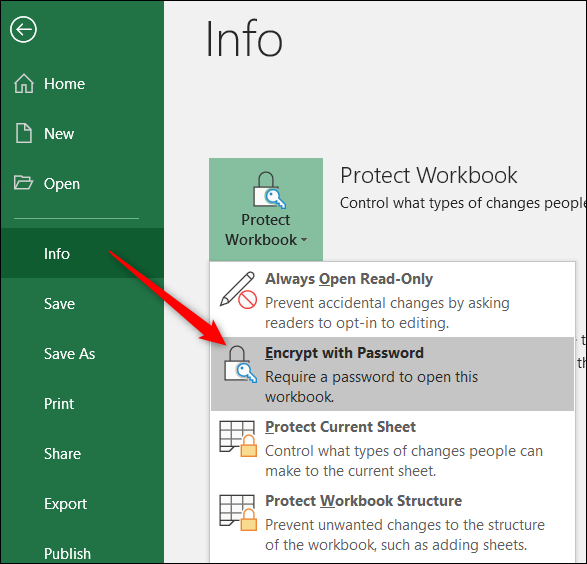
- In the opened window of Encrypt Document, just enter the password which you want to set. After that click to the ok.

Note: read the caution lines carefully and set the password that you don’t forget.
- For the password confirmation, you are asked to enter the password two times. After that click the OK button.

- To check whether your Excel workbook gets encrypted properly or not, You need to close your already opened workbook and re-open it again.

If later on, you want to remove password from Excel workbook then follow the steps given in this tutorial: Top 3 Methods To Unlock Password Protected Excel File
2. Make A Workbook Read-Only
Making Excel workbook read-only is very easy. This option doesn’t give any real protection so any user who is opening the file can easily enable the editing option. But it will give suggestions to the other user for being careful while making changes in the file.
- At first, Open your Excel workbook which you want to make read-only.
- Now Go to the file > info> Protect Workbook.
- Now from the drop-down options of Protect Workbook choose the “always open read only”.

- After applying this, whenever anyone tries to open the Excel file, they will get the warning that the file is opened in read-only mode.

- For removing up this read-only setting, just go to the File > Protect Workbook Now toggle the “Always Open Read-Only” setting off.
Helpful Article: 7 Quick Ways To Fix Excel File Read Only Error
Trick 3# Protect Excel Worksheet From Editing
Another option of preventing Excel workbook from editing is by protecting each individual worksheet.
Using this option you can easily lock all the cells from being edited by anyone. Protect Excel Worksheet means no can edit or delete its content.
Follow the below steps to Protect Excel Worksheet From Editing:
- From the Excel ribbon tap to the “Review” tab.
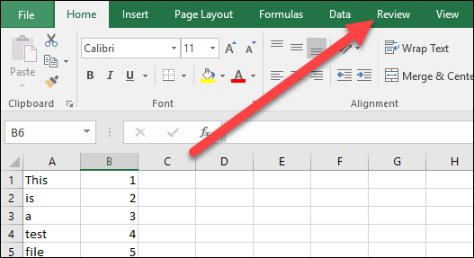
- Now from the changes group make a tap on the “Protect Sheet.”

- Assign the password which you want to set for unlocking your Excel sheet in the future again.

- Enter the password one more time to make a confirmation and hit the ok.
- Choose the permissions from the listed option of “allow all users of this worksheet to” and then click the ok.
- For removing up the protection, go to the “Review” tab and hit the button “Unprotect Sheet”.
- Enter the password and click the “OK” button.

- Now your sheet is unprotected. So you have to apply for the protection again whenever you need it.
Trick 4# Protect Excel Workbook’s Structure From Editing
Another option to prevent workbook from editing is by protecting the Excel workbook’s structure.
Follow the steps to Protect Excel Workbook’s Structure From Editing:
- Go to the File menu in your opened Excel file. After that click on the following: Info> Protect Workbook> protect workbook structure.

- Assign the password and click the “OK”.

- Re-enter the password again for confirmation and click “OK.”
- After applying this option, anyone can open your Excel document but they can’t access its structural commands.
- If another user knows your password, they can easily access these commands. Only they need to make click over the “Review” tab and tap on the “Protect Workbook”.
- After that, they have to enter the password and now the structural commands get available.

This action will remove your Excel workbook structure protection from the document. For restating it, just go back to the File menu and protect your workbook once more.
Trick 5# Protect Excel Cells From Editing
If you want to protect only specific cells of your Excel sheet from editing then locking those cells is the best option.
Apply the following steps to protect specific cells from editing:
- Choose the cells which you want to lock from editing.

- Now, make a right-click over your selected cells. After that choose the command “Format Cells”.
- In the Format Cells window, go to the “Protection”.

- Uncheck the checkbox present across the “Locked”.

- Hit the ok.

Helpful article: How To Lock And Unlock Cells, Formulas In Microsoft Excel 2016?
What Happens When You Protect A Workbook In Excel?
Protecting a workbook in Excel is basically used for controlling the access of another user within the workbook structure.
Excel workbook protection isn’t the security feature and you can’t use it as a means of protection for your intellectual property.
This option forbids other users from making any changes in the worksheets and also makes a strong defense against the hidden worksheets.
As there are so many Excel password remover tools available. So it’s that tough for any user to crack your password and edit your workbook.
It’s better to keep a backup of all your work before giving it to other users.
What Is The Difference Between Protect Sheet And Protect Workbook In Excel?
- Workbook-level:
With the application of this Workbook-level security you can lock the workbook structure by setting up the password. Locking up workbook structure prevent third party user from hiding, renaming, adding, moving the Excel worksheets.
- Worksheet-level:
Whereas with the application of worksheet level protection, you can easily keep control of other users working styles within your worksheets. As you have the option to specify what other users can do in the Excel worksheet.
Thus it assures you that none of your worksheet important data gets affected.
Suppose, if you want that the user will only add columns and rows or can only sort or use the auto filters. In that case, once you enable the sheet protection, you can easily protect other elements like ranges, formulas, cells, and ActiveX or Form controls.
How To Retrieve Lost Or Deleted Excel Workbook Data?
Following the above-given tricks, you can easily protect Excel workbooks from editing. But if due to misdeeds of any other user you get stuck into worksheet corruption, deletion, or missing like situations.
In that case, also you have the option left, so don’t get worried…!
It is recommended to try the Excel Repair Tool for easy repair and recovery of corrupted, damaged, and inaccessible data from the Excel workbook. This tool is well capable of fixing different errors and issues related to the Excel workbook and recover deleted Excel data.
* Free version of the product only previews recoverable data.
With this unique tool, you can restore entire data including the charts, worksheet properties cell comments, and other data without doing any modification. It is easy to use and support all Excel versions.
So, try the given solutions to recover corrupted Excel workbook data.
Wrap Up:
You have the option to use one or more protection levels in your Excel workbook s per your requirements.
Using all the options to protect Excel workbook from editing is completely depends on the security level which you want to apply for your Excel data.
You can opt for encrypting your shared Excel file along with enabling the worksheet or workbook protection. If you are applying the worksheet protection feature on your personal workbook to safeguard Excel formulas from deletion.
If, in case you have any additional questions concerning the ones presented, do tell us in the comments section below or you can also visit our Repair MS Excel social account Facebook and Twitter page.
Good Luck….


Priyanka is an entrepreneur & content marketing expert. She writes tech blogs and has expertise in MS Office, Excel, and other tech subjects. Her distinctive art of presenting tech information in the easy-to-understand language is very impressive. When not writing, she loves unplanned travels.
Microsoft Excel предоставляет пользователю несколько, условно выражаясь, уровней защиты — от простой защиты отдельных ячеек до шифрования всего файла шифрами крипто-алгоритмов семейства RC4. Разберем их последовательно…
Уровень 0. Защита от ввода некорректных данных в ячейку
Самый простой способ. Позволяет проверять что именно пользователь вводит в определенные ячейки и не разрешает вводить недопустимые данные (например, отрицательную цену или дробное количество человек или дату октябрьской революции вместо даты заключения договора и т.п.) Чтобы задать такую проверку ввода, необходимо выделить ячейки и выбрать на вкладке Данные (Data) кнопку Проверка данных (Data Validation). В Excel 2003 и старше это можно было сделать с помощью меню Данные — Проверка (Data — Validation). На вкладке Параметры из выпадающего списка можно выбрать тип разрешенных к вводу данных:

Соседние вкладки этого окна позволяют (при желании) задать сообщения, которые будут появляться перед вводом — вкладка Сообщение для ввода (Input Message), и в случае ввода некорректной информации — вкладка Сообщение об ошибке (Error Alert):

Уровень 1. Защита ячеек листа от изменений
Мы можем полностью или выборочно запретить пользователю менять содержимое ячеек любого заданного листа. Для установки подобной защиты следуйте простому алгоритму:
- Выделите ячейки, которые не надо защищать (если таковые есть), щелкните по ним правой кнопкой мыши и выберите в контекстном меню команду Формат ячеек (Format Cells). На вкладке Защита (Protection) снимите флажок Защищаемая ячейка (Locked). Все ячейки, для которых этот флажок останется установленным, будут защищены при включении защиты листа. Все ячейки, где вы этот флаг снимете, будут доступны для редактирования несмотря на защиту. Чтобы наглядно видеть, какие ячейки будут защищены, а какие — нет, можно воспользоваться этим макросом.
- Для включения защиты текущего листа в Excel 2003 и старше — выберите в меню Сервис — Защита — Защитить лист (Tools — Protection — Protect worksheet), а в Excel 2007 и новее — нажмите кнопку Защитить лист (Protect Sheet) на вкладке Рецензирование (Reveiw). В открывшемся диалоговом окне можно задать пароль (он будет нужен, чтобы кто попало не мог снять защиту) и при помощи списка флажков настроить, при желании, исключения:

Т.е., если мы хотим оставить пользователю возможность, например, форматировать защищенные и незащищенные ячейки, необходимо установить первых три флажка. Также можно разрешить пользователям использовать сортировку, автофильтр и другие удобные средства работы с таблицами.
Уровень 2. Выборочная защита диапазонов для разных пользователей
Если предполагается, что с файлом будут работать несколько пользователей, причем каждый из них должен иметь доступ в свою область листа, то можно установить защиту листа с разными паролями на разные диапазоны ячеек.
Чтобы сделать это выберите на вкладке Рецензирование (Review) кнопку Разрешить изменение диапазонов (Allow users edit ranges). В версии Excel 2003 и старше для этого есть команда в меню Сервис — Защита — Разрешить изменение диапазонов (Tools — Protection — Allow users to change ranges):

В появившемся окне необходимо нажать кнопку Создать (New) и ввести имя диапазона, адреса ячеек, входящих в этот диапазон и пароль для доступа к этому диапазону:

Повторите эти действия для каждого из диапазонов разных пользователей, пока все они не окажутся в списке. Теперь можно нажать кнопку Защитить лист (см. предыдущий пункт) и включить защиту всего листа.
Теперь при попытке доступа к любому из защищенных диапазонов из списка, Excel будет требовать пароль именно для этого диапазона, т.е. каждый пользователь будет работать «в своем огороде».
Уровень 3. Защита листов книги
Если необходимо защититься от:
- удаления, переименования, перемещения листов в книге
- изменения закрепленных областей («шапки» и т.п.)
- нежелательных изменений структуры (сворачивание строк/столбцов при помощи кнопок группировки «плюс/минус»)
- возможности сворачивать/перемещать/изменять размеры окна книги внутри окна Excel
то вам необходима защита всех листов книги, с помощью кнопки Защитить книгу (Protect Workbook) на вкладке Рецензирование (Reveiw) или — в старых версиях Excel — через меню Сервис — Защита — Защитить книгу (Tools — Protection — Protect workbook):

Уровень 4. Шифрование файла
При необходимости, Excel предоставляет возможность зашифровать весь файл книги, используя несколько различных алгоритмов шифрования семейства RC4. Такую защиту проще всего задать при сохранении книги, т.е. выбрать команды Файл — Сохранить как (File — Save As), а затем в окне сохранения найти и развернуть выпадающий список Сервис — Общие параметры (Tools — General Options). В появившемся окне мы можем ввести два различных пароля — на открытие файла (только чтение) и на изменение:

Ссылки по теме
- Как установить/снять защиту на все листы книги сразу (надстройка PLEX)
- Подсветка незащищенных ячеек цветом
- Правильная защита листов макросом
Sometimes we want our sheets to be view only. We don’t want the user to make any change to some specific sheet. In that case, we should protect or say lock our sheets for the editing. Luckily, excel provides these features in the Review section of the ribbon.

How to protect an Excel sheet with a password?
It is useless (in most cases) to protect a sheet, without a password. Anyone can go to the Review section and unprotect your protected sheet easily. Follow these steps to put a password on an Excel sheet.
- Go to Review, and click on the Protect Sheet. Protect sheet dialog will open.
- On the top of the dialog box, it asks for a password. Type the password and hit OK. It will again ask you for the same password to ensure you have entered the intended password. Enter the same password again.

- Hit ok.
Note: The password is case sensitive always.
Now the sheet is protected. If you try to write anything on the sheet, Excel won’t allow you. But you can still select and copy data. We restrict that too.
Restricting User from Copying Data from Excel Sheet
When you click on Protect Sheet, the dialog box opens. This dialog box has a list with heading as «Allow all users of this worksheet to:». This list contains the task the user can do. Every checked item can be performed by the user, even if the sheet is protected.
Now, if you want the user to not be able to select and copy any data:
- Uncheck the «select locked cells» and «select unlocked cells» option. (by default, only these options are checked)
Now the user can only view this sheet. Users can’t select any cell or do anything on this sheet.
So yeah guys, this how you can protect or lock your excel sheets. I hope it was helpful. If you have any doubt or specific query related to protecting sheet or any Excel/VBA related query, ask in the comments section below.
Related Articles:
Protecting Cells Containing Formulas in Protected Sheet | To protect the formulas from the end-users, we lock the cells first. Then…
Protecting Workbooks with a Digital Signature | Protect your workbook with your digital signature. Here’s how…
Protect and Unprotect Excel Workbooks | To protect excel workbooks with a password with a read-only option or to put opening restrictions use this method.
Popular Articles:
50 Excel Shortcuts to Increase Your Productivity | Get faster at your task. These 50 shortcuts will make you work even faster on Excel.
The VLOOKUP Function in Excel | This is one of the most used and popular functions of excel that is used to lookup value from different ranges and sheets.
COUNTIF in Excel 2016 | Count values with conditions using this amazing function. You don’t need filter your data to count specific value. Countif function is essential to prepare your dashboard.
How to Use SUMIF Function in Excel | This is another dashboard essential function. This helps you sum up values on specific conditions.