Sheet function in excel

Excel for Microsoft 365 Excel for Microsoft 365 for Mac Excel for the web Excel 2021 Excel 2021 for Mac Excel 2019 Excel 2019 for Mac Excel 2016 Excel 2016 for Mac Excel 2013 More…Less

This article describes the formula syntax and usage of the SHEETS
 function in Microsoft Excel.

Description

Returns the number of sheets in a reference.

Syntax

SHEETS(reference)

The SHEETS function syntax has the following arguments.

  • Reference    Optional. Reference is a reference for which you want to know the number of sheets it contains. If Reference is omitted, SHEETS returns the number of sheets in the workbook that contains the function.

Remarks

  • SHEETS includes all worksheets (visible, hidden, or very hidden) in addition to all other sheet types (macro, chart, or dialog sheets).

  • If reference is not a valid value, SHEETS returns the #REF! error value.

  • SHEETS is not available in the Object Model (OM) because the Object Model already includes similar functionality.

Example

Copy the example data in the following table, and paste it in cell A1 of a new Excel worksheet. For formulas to show results, select them, press F2, and then press Enter. If you need to, you can adjust the column widths to see all the data.

Formula

Description

Result

=SHEETS()

Because there is no Reference argument specified, the total number of sheets in the workbook is returned (3).

3

=SHEETS(My3DRef)

Returns the number of sheets in a 3D reference with the defined name My3DRef, which includes Sheet2 and Sheet3 (2).

2

Top of Page

Need more help?

Want more options?

Explore subscription benefits, browse training courses, learn how to secure your device, and more.

Communities help you ask and answer questions, give feedback, and hear from experts with rich knowledge.

SHEET function in Excel returns a numeric value corresponding to the sheet number referenced by the link passed to the function as a parameter.


SHEET and SHEETS functions in Excel: description of arguments and syntax

SHEETS function in Excel returns a numeric value that corresponds to the number of sheets referenced.

Notes:

  1. Both functions are useful for use in documents containing a large number of sheets.
  2. A sheet in Excel is a table of all the cells that are displayed on the screen and are outside of it (a total of 1,048,576 rows and 16,384 columns). When sending a sheet to print, it can be divided into several pages. Therefore, the terms “sheet” and “page” should not be confused.
  3. The number of sheets in the book is limited only by the amount of PC RAM.

Function has only 1 argument in its syntax and is optional for: =SHEET(value).

  • value is an optional function argument that contains text data with the name of the sheet or a link for which you want to set the sheet number. If this parameter is not specified, the function will return the number of the sheet in one of the cells of which it was written.

Notes:

  1. When the sheet works, all sheets that are visible, hidden and very hidden are taken into account. Exceptions are dialogs, macros, and diagrams.
  2. If the function argument is a text value that does not match the name of any of the sheets contained in the book, the error #NA will be returned.
  3. If an invalid value was passed as an argument to the function, the result of its calculation will be the error #REF!.
  4. Within the object model (the hierarchy of objects in VBA, in which Application is the main object and Workbook, WorkSheet, etc., are child objects), the SHEET function is not available because it contains a similar function.

The function has the following syntax: =SHEETS(reference).

  • reference — an object of reference type for which you want to determine the number of sheets. This argument is optional. If this parameter is not specified, the function will return the number of sheets contained in the book where it was written.

Notes:

  1. This function counts the number of all hidden, very hidden and visible sheets, with the exception of charts, macros and dialogs.
  2. If an invalid reference was passed as a parameter, the result of the calculation is the error code #REF!.
  3. This function is not available in the object model due to the presence of a similar function there.


How to get sheet name by formula in Excel

Example 1. In carrying out the calculated work the student used the Excel program, in which he created a book of several sheets. For his own convenience, the student decided to display in the cells A2 and B2 of each sheet data on the name of the sheet and its serial number, respectively. For this, he used the following formulas:

Example 1.

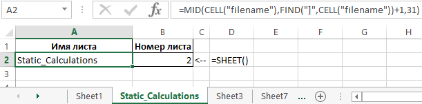
Description of arguments for the MID function:

  1. =CELL(«filename») is a function that returns text in which the MID function searches for a specified number of characters. In this case, the value “C:UserssoulpDesktop[Workbook.xlsx] Static_Calculations” will return, where after the “]” symbol is the required text — the name.
  2. =FIND(«]»,CELL(«filename»))+1 is a function that returns the position number of the character «]», one is added so that the MID function does not take into account the character].
  3. 31 — the maximum number of characters in the name.

=SHEET() — this function without parameter returns the number of the current sheet. As a result of its calculation, we get the number of sheets in the current book.

Examples of using the SHEET function and SHEETS

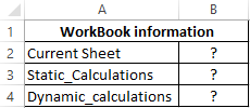
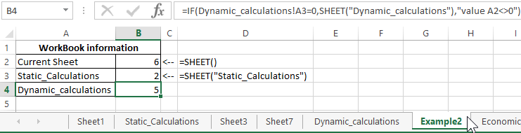
Example 2. The Excel workbook contains several sheets. It is necessary:

  1. Return the current sheet number.
  2. Return the sheet number with the name «Static_calculations».
  3. Return the number of the sheet «Dynamic_calculations», if its cell A3 contains the value 0.

Enter the data in the table:

Example 2.

Next, we write the formulas for all 4 conditions:

  • For condition # 1, use the following formula: =SHEET()
  • For condition # 2, enter the formula: =SHEET(«Static_calculations»)
  • For condition number 3 we write the formula:

The IF function checks whether the value stored in the A3 cell of the Dynamic_ calculations is equal to zero or null.

As a result, we get:

.

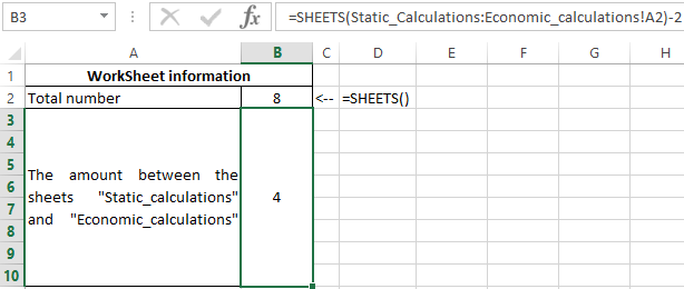
Processing information about the sheets of the book on the formula Excel

Example 3. To determine the contains several sheets. It is necessary to determine the total number of sheets, as well as the number contained between the “Static_calculations” and “Economic_calculations”.

The source table is:

.

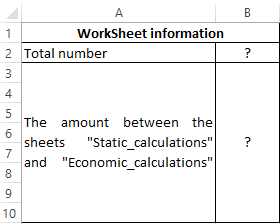
The total number of sheets is calculated by the formula:

To determine the number contained between these two sheets, we write the formula:

  1. Static_calculations: Economic_calculations!A2 — A reference to cell A2 of the range of sheets between «Static_calculations» and «Economic_calculations» including these sheets.
  2. To get the desired value, 2 was subtracted.

As a result, we get the following:

.

Download examples SHEET and SHEETS functions in Excel formulas

The formula displays detailed information on the data on the sheets in a certain range of their location in the Excel workbook.


In this article, we will learn about how to use the SHEET function in Excel. 

What is the SHEET function?

SHEET function in excel is a built-in reference function. This function returns a number, reference to the input sheet indicated. SHEET function can be used for the following purposes in Excel.

  1. The function returns the total number of sheets in the current worksheet.
  2. The function returns the sheet number of the reference sheet cell.
  3. The function returns the sheet number for the reference table in the worksheet.

What is the SHEET function?

SHEET function in excel returns SHEET number for the reference value.

Syntax of SHEET function:

= SHEET ( value )

value : value be given using cell reference
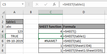
Example:

All of these might be confusing to understand. So, let’s test this formula via running it on the example shown below. Here we have some random data values to test the SHEET function in Excel.

Here we have some different uses of SHEET function and we need to get the Sheet number in number format .using the below formula

Use the formula:

=SHEET()

Or

=SHEET(table1)

Where table1 is name given to the table using the named range in Excel.

As you can see the formula returns error if the table name is not defined.

Here are some observational notes shown below.

Notes:

  1. The formula returns the sheet number of the input reference cell.
  2. If the sheet array is given as cell reference, the formula returns the first sheet number.
  3. Use the SHEETS function to count the number of sheet if the range of sheet is given as input.

Hope this article about How to use the SHEET function in Excel is explanatory. Find more articles on the SHEETS function here. If you liked our blogs, share it with your fristarts on Facebook. And also you can follow us on Twitter and Facebook. We would love to hear from you, do let us know how we can improve, complement or innovate our work and make it better for you. Write to us at T@exceltip.com.

Related Articles

How to use the CELL function in Excel : returns Information about a cell in a worksheet using the CELL function.

How to use the TYPE Function in Excel : returns numeric code representing the TYPE of data using TYPE function in Excel.

How to use the SHEETS function in Excel : returns a number, reference to input sheet indicated using the SHEETS function.

How to Use ISNUMBER Function in Excel : ISNUMBER function returns TRUE if number or FALSE if not in Excel. 

Popular Articles:

50 Excel Shortcuts to Increase Your Productivity | Get faster at your task. These 50 shortcuts will make you work even faster on Excel.

The VLOOKUP Function in Excel | This is one of the most used and popular functions of excel that is used to lookup value from different ranges and sheets. 

COUNTIF in Excel 2016 | Count values with conditions using this amazing function. You don’t need to filter your data to count specific values. Countif function is essential to prepare your dashboard.

How to Use SUMIF Function in Excel | This is another dashboard essential function. This helps you sum up values on specific conditions.

Date yes Add (Subtract) Days to a Date Concatenate Dates Convert Date to Number Convert Date to Text Month Name to Number Create Date Range from Dates Day Number of Year Month Name from Date First Day of Month Add (Subtract) Weeks to a Date If Functions with Dates Max Date Number of Days Between Dates Number of Days in a Month Number of Weeks Between Dates Number of Years Between Dates Split Date & Time into Separate Cells Countdown Remaining Days Insert Dates Random Date Generator Using Dynamic Ranges — Year to Date Values Add (Subtract) Years to a Date Date Formula Examples Extract Day from Date Get Day Name from Date Count Days Left in Month / Year Count Workdays Left in Month / Year Get Last Day of Month Last Business Day of Month / Year Number of Work / Business Days in Month Weekday Abbreviations Auto Populate Dates Number of Months Between Dates Quarter from a Date Years of Service Change Date Format Compare Dates Time yes Add (Subtract) Hours to Time Add (Subtract) Minutes to Time Add (Subtract) Seconds to Time Add Up time (Total Time) Time Differences Change Time Format Convert Minutes to Hours Convert Time to Decimal Convert Time to Hours Convert Time to Minutes Convert Time to Seconds Military Time Round Time to Nearest 15 Minutes Overtime Calculator Number of Hours Between Times Convert Seconds to Minutes, Hours, or Time Count Hours Worked Time Differences Time Format — Show Minutes Seconds Text yes Add Commas to Cells Get First Word from Text Capitalize First Letter Clean & Format Phone #s Remove Extra Trailing / Leading Spaces Add Spaces to Cell Assign Number Value to Text Combine Cells with Comma Combine First and Last Names Convert Text String to Date Convert Text to Number Extract Text From Cell Get Last Word Remove Unwated Characters Extract Text Before or After Character How to Split Text String by Space, Comma, & More Remove Special Characters Remove First Characters from Left Substitute Multiple Values Switch First & Last Names w/ Commas Remove Specific Text from a Cell Extract Text Between Characters (Ex. Parenthesis) Add Leading Zeros to a Number Remove Line Breaks from Text Remove all Numbers from Text Reverse Text Remove Non-Numeric Characters Remove Last Character(s) From Right Separate First and Last Names Separate Text & Numbers Round yes Round Formulas Round Price to Nearest Dollar or Cent Round to Nearest 10, 100, or 1000 Round to Nearest 5 or .5 Round Percentages Round to Significant Figures Count yes Count Blank and Non-blank Cells Count Cells Between Two Numbers Count Cells not Equal to Count if Cells are in Range Count Times Word Appears in Cell Count Words in Cell Count Specific Characters in Column Count Total Number of Characters in Column Count Cells that Equal one of two Results Count Cells that do not Contain Count Cells that Contain Specific Text Count Unique Values in Range Countif — Multiple Criteria Count Total Number of Cells in Range Count Cells with Any Text Count Total Cells in a Table Lookup yes Two Dimensional VLOOKUP VLOOKUP Simple Example Vlookup — Multiple Matches Case Sensitive Lookup Case Sensitive VLOOKUP Sum if — VLOOKUP Case Sensitive Lookup Case Sensitive VLOOKUP Find Duplicates w/ VLOOKUP or MATCH INDEX MATCH MATCH Lookup — Return Cell Address (Not Value) Lookup Last Value in Column or Row Reverse VLOOKUP (Right to Left) Risk Score Bucket with VLOOKUP Sum with a VLOOKUP Function VLOOKUP & INDIRECT VLOOKUP Concatenate VLOOKUP Contains (Partial Match) 17 Reasons Why Your XLOOKUP is Not Working Double (Nested) XLOOKUP — Dynamic Columns IFERROR (& IFNA) XLOOKUP Lookup Min / Max Value Nested VLOOKUP Top 11 Alternatives to VLOOKUP (Updated 2022!) VLOOKUP – Dynamic Column Reference VLOOKUP – Fix #N/A Error VLOOKUP – Multiple Sheets at Once VLOOKUP & HLOOKUP Combined VLOOKUP & MATCH Combined VLOOKUP Between Worksheets or Spreadsheets VLOOKUP Duplicate Values VLOOKUP Letter Grades VLOOKUP Return Multiple Columns VLOOKUP Returns 0? Return Blank Instead VLOOKUP w/o #N/A Error XLOOKUP Multiple Sheets at Once XLOOKUP Between Worksheets or Spreadsheets XLOOKUP by Date XLOOKUP Duplicate Values XLOOKUP Multiple Criteria XLOOKUP Return Multiple Columns XLOOKUP Returns 0? Return Blank Instead XLOOKUP Text XLOOKUP with IF XLOOKUP With If Statement Misc. yes Sort Multiple Columns Use Cell Value in Formula Percentage Change Between Numbers Percentage Breakdown Rank Values Add Spaces to Cell CAGR Formula Average Time Decimal Part of Number Integer Part of a Number Compare Items in a List Dealing with NA() Errors Get Worksheet Name Wildcard Characters Hyperlink to Current Folder Compound Interest Formula Percentage Increase Create Random Groups Sort with the Small and Large Functions Non-volatile Function Alternatives Decrease a Number by a Percentage Calculate Percent Variance Profit Margin Calculator Convert Column Number to Letter Get Full Address of Named Range Insert File Name Insert Path Latitute / Longitude Functions Replace Negative Values Reverse List Range Convert State Name to Abbreviation Create Dynamic Hyperlinks Custom Sort List with Formula Data Validation — Custom Formulas Dynamic Sheet Reference (INDIRECT) Reference Cell in Another Sheet or Workbook Get Cell Value by Address Get Worksheet Name Increment Cell Reference List Sheet Names List Skipped Numbers in Sequence Return Address of Max Value in Range Search by Keywords Select Every Other (or Every nth) Row Basics yes Cell Reference Basics — A1, R1C1, 3d, etc. Add Up (Sum) Entire Column or Row Into to Dynamic Array Formulas Conversions yes Convert Time Zones Convert Celsius to Fahrenheit Convert Pounds to Kilograms Convert Time to Unix Time Convert Feet to Meters Convert Centimeters to Inches Convert Kilometers to Miles Convert Inches to Feet Convert Date to Julian Format Convert Column Letter to Number Tests yes Test if a Range Contains any Text Test if any Cell in Range is Number Test if a Cell Contains a Specific Value Test if Cell Contains Any Number Test if Cell Contains Specific Number Test if Cell is Number or Text If yes Percentile If Subtotal If Sumproduct If Large If and Small If Median If Concatentate If Max If Rank If TEXTJOIN If Sum yes Sum if — Begins With / Ends With Sum if — Month or Year to Date Sum if — By Year Sum if — Blank / Non-Blank Sum if — Horizontal Sum Count / Sum If — Cell Color INDIRECT Sum Sum If — Across Multiple Sheets Sum If — By Month Sum If — Cells Not Equal To Sum If — Not Blank Sum if — Between Values Sum If — Week Number Sum Text Sum if — By Category or Group Sum if — Cell Contains Specific Text (Wildcards) Sum if — Date Rnage Sum if — Dates Equal Sum if — Day of Week Sum if — Greater Than Sum if — Less Than Average yes Average Non-Zero Values Average If — Not Blank Average — Ignore 0 Average — Ignore Errors Math yes Multiplication Table Cube Roots nth Roots Square Numbers Square Roots Calculations yes Calculate a Ratio Calculate Age KILLLLLLL Calculate Loan Payments GPA Formula Calculate VAT Tax How to Grade Formulas Find yes Find a Number in a Column / Workbook Find Most Frequent Numbers Find Smallest n Values Find nth Occurance of Character in Text Find and Extract Number from String Find Earliest or Latest Date Based on Criteria Find First Cell with Any Value Find Last Row Find Last Row with Data Find Missing Values Find Largest n Values Most Frequent Number Conditional Formatting yes Conditional Format — Dates & Times Conditional Format — Highlight Blank Cells New Functions XLOOKUP Replaces VLOOKUP, HLOOKUP, and INDEX / MATCH Logical yes AND Checks whether all conditions are met. TRUE/FALSE IF If condition is met, do something, if not, do something else. IFERROR If result is an error then do something else. NOT Changes TRUE to FALSE and FALSE to TRUE. OR Checks whether any conditions are met. TRUE/FALSE XOR Checks whether one and only one condition is met. TRUE/FALSE Lookup & Reference yes FALSE The logical value: FALSE. TRUE The logical value: TRUE. ADDRESS Returns a cell address as text. AREAS Returns the number of areas in a reference. CHOOSE Chooses a value from a list based on it’s position number. COLUMN Returns the column number of a cell reference. COLUMNS Returns the number of columns in an array. HLOOKUP Lookup a value in the first row and return a value. HYPERLINK Creates a clickable link. INDEX Returns a value based on it’s column and row numbers. INDIRECT Creates a cell reference from text. LOOKUP Looks up values either horizontally or vertically. MATCH Searches for a value in a list and returns its position. OFFSET Creates a reference offset from a starting point. ROW Returns the row number of a cell reference. ROWS Returns the number of rows in an array. TRANSPOSE Flips the oriention of a range of cells. VLOOKUP Lookup a value in the first column and return a value. Date & Time yes DATE Returns a date from year, month, and day. DATEDIF Number of days, months or years between two dates. DATEVALUE Converts a date stored as text into a valid date DAY Returns the day as a number (1-31). DAYS Returns the number of days between two dates. DAYS360 Returns days between 2 dates in a 360 day year. EDATE Returns a date, n months away from a start date. EOMONTH Returns the last day of the month, n months away date. HOUR Returns the hour as a number (0-23). MINUTE Returns the minute as a number (0-59). MONTH Returns the month as a number (1-12). NETWORKDAYS Number of working days between 2 dates. NETWORKDAYS.INTL Working days between 2 dates, custom weekends. NOW Returns the current date and time. SECOND Returns the second as a number (0-59) TIME Returns the time from a hour, minute, and second. TIMEVALUE Converts a time stored as text into a valid time. TODAY Returns the current date. WEEKDAY Returns the day of the week as a number (1-7). WEEKNUM Returns the week number in a year (1-52). WORKDAY The date n working days from a date. WORKDAY.INTL The date n working days from a date, custom weekends. YEAR Returns the year. YEARFRAC Returns the fraction of a year between 2 dates. Engineering yes CONVERT Convert number from one unit to another. Financial yes FV Calculates the future value. PV Calculates the present value. NPER Calculates the total number of payment periods. PMT Calculates the payment amount. RATE Calculates the interest Rate. NPV Calculates the net present value. IRR The internal rate of return for a set of periodic CFs. XIRR The internal rate of return for a set of non-periodic CFs. PRICE Calculates the price of a bond. YIELD Calculates the bond yield. INTRATE The interest rate of a fully invested security. Information yes CELL Returns information about a cell. ERROR.TYPE Returns a value representing the cell error. ISBLANK Test if cell is blank. TRUE/FALSE ISERR Test if cell value is an error, ignores #N/A. TRUE/FALSE ISERROR Test if cell value is an error. TRUE/FALSE ISEVEN Test if cell value is even. TRUE/FALSE ISFORMULA Test if cell is a formula. TRUE/FALSE ISLOGICAL Test if cell is logical (TRUE or FALSE). TRUE/FALSE ISNA Test if cell value is #N/A. TRUE/FALSE ISNONTEXT Test if cell is not text (blank cells are not text). TRUE/FALSE ISNUMBER Test if cell is a number. TRUE/FALSE ISODD Test if cell value is odd. TRUE/FALSE ISREF Test if cell value is a reference. TRUE/FALSE ISTEXT Test if cell is text. TRUE/FALSE N Converts a value to a number. NA Returns the error: #N/A. TYPE Returns the type of value in a cell. Math yes ABS Calculates the absolute value of a number. AGGREGATE Define and perform calculations for a database or a list. CEILING Rounds a number up, to the nearest specified multiple. COS Returns the cosine of an angle. DEGREES Converts radians to degrees. DSUM Sums database records that meet certain criteria. EVEN Rounds to the nearest even integer. EXP Calculates the exponential value for a given number. FACT Returns the factorial. FLOOR Rounds a number down, to the nearest specified multiple. GCD Returns the greatest common divisor. INT Rounds a number down to the nearest integer. LCM Returns the least common multiple. LN Returns the natural logarithm of a number. LOG Returns the logarithm of a number to a specified base. LOG10 Returns the base-10 logarithm of a number. MOD Returns the remainder after dividing. MROUND Rounds a number to a specified multiple. ODD Rounds to the nearest odd integer. PI The value of PI. POWER Calculates a number raised to a power. PRODUCT Multiplies an array of numbers. QUOTIENT Returns the integer result of division. RADIANS Converts an angle into radians. RAND Calculates a random number between 0 and 1. RANDBETWEEN Calculates a random number between two numbers. ROUND Rounds a number to a specified number of digits. ROUNDDOWN Rounds a number down (towards zero). ROUNDUP Rounds a number up (away from zero). SIGN Returns the sign of a number. SIN Returns the sine of an angle. SQRT Calculates the square root of a number. SUBTOTAL Returns a summary statistic for a series of data. SUM Adds numbers together. SUMIF Sums numbers that meet a criteria. SUMIFS Sums numbers that meet multiple criteria. SUMPRODUCT Multiplies arrays of numbers and sums the resultant array. TAN Returns the tangent of an angle. TRUNC Truncates a number to a specific number of digits. Stats yes AVERAGE Averages numbers. AVERAGEA Averages numbers. Includes text & FALSE =0, TRUE =1. AVERAGEIF Averages numbers that meet a criteria. AVERAGEIFS Averages numbers that meet multiple criteria. CORREL Calculates the correlation of two series. COUNT Counts cells that contain a number. COUNTA Count cells that are non-blank. COUNTBLANK Counts cells that are blank. COUNTIF Counts cells that meet a criteria. COUNTIFS Counts cells that meet multiple criteria. FORECAST Predict future y-values from linear trend line. FREQUENCY Counts values that fall within specified ranges. GROWTH Calculates Y values based on exponential growth. INTERCEPT Calculates the Y intercept for a best-fit line. LARGE Returns the kth largest value. LINEST Returns statistics about a trendline. MAX Returns the largest number. MEDIAN Returns the median number. MIN Returns the smallest number. MODE Returns the most common number. PERCENTILE Returns the kth percentile. PERCENTILE.INC Returns the kth percentile. Where k is inclusive. PERCENTILE.EXC Returns the kth percentile. Where k is exclusive. QUARTILE Returns the specified quartile value. QUARTILE.INC Returns the specified quartile value. Inclusive. QUARTILE.EXC Returns the specified quartile value. Exclusive. RANK Rank of a number within a series. RANK.AVG Rank of a number within a series. Averages. RANK.EQ Rank of a number within a series. Top Rank. SLOPE Calculates the slope from linear regression. SMALL Returns the kth smallest value. STDEV Calculates the standard deviation. STDEV.P Calculates the SD of an entire population. STDEV.S Calculates the SD of a sample. STDEVP Calculates the SD of an entire population TREND Calculates Y values based on a trendline. Text yes CHAR Returns a character specified by a code. CLEAN Removes all non-printable characters. CODE Returns the numeric code for a character. CONCATENATE Combines text together. DOLLAR Converts a number to text in currency format. EXACT Test if cells are exactly equal. Case-sensitive. TRUE/FALSE FIND Locates position of text within a cell.Case-sensitive. LEFT Truncates text a number of characters from the left. LEN Counts number of characters in text. LOWER Converts text to lower case. MID Extracts text from the middle of a cell. PROPER Converts text to proper case. REPLACE Replaces text based on it’s location. REPT Repeats text a number of times. RIGHT Truncates text a number of characters from the right. SEARCH Locates position of text within a cell.Not Case-sensitive. SUBSTITUTE Finds and replaces text. Case-sensitive. TEXT Converts a value into text with a specific number format. TRIM Removes all extra spaces from text. UPPER Converts text to upper case. VALUE Converts a number stored as text into a number.

Функция ЛИСТ возвращает номер листа, на значения которого ссылается функция. Впервые функция была представлена в Excel 2013.

Описание функции ЛИСТ

Возвращает номер листа, на значения которого ссылается функция.

Синтаксис

=ЛИСТ(значение)

Аргументы

значение

Необязательный аргумент. Значение — это название листа или ссылка, для которой необходимо установить номер листа. Если опустить значение, функция ЛИСТ вернет номер листа, который содержит функцию.

Замечания

  • Функция ЛИСТ включает в себя все листы (видимые, скрытые или очень скрытые), кроме всех остальных типов листов (макросов, диаграмм или диалогов).
  • Если аргумент значения не является действительным значением, функция ЛИСТ возвращает значение ошибки #ССЫЛКА!. Например, =ЛИСТ(Лист1!#ССЫЛКА) вернет значение ошибки #ССЫЛКА!.
  • Если аргумент значения является названием недействительного листа, функция ЛИСТ вернет значение ошибки #НД. Например, =ЛИСТ(«badЛИСТName») вернет значение ошибки #НД.
  • Функция ЛИСТ недоступна в объектной модели (OM), поскольку там уже содержится похожая функция.

Пример

Видео работы функции

Использование ЛИСТ и ЛИСТЫ (англ.)

The Excel SHEET function, new in Excel 2013, returns the sheet number of the referenced sheet based on its position in the file. It can return the sheet number of any worksheet including visible, hidden or very hidden as well as macro, chart and dialog sheets.

SHEET function syntax:

=SHEET(value)

Where value is the name of the sheet or reference you want the sheet number of. The value can include cell references, named ranges or Table names.

You can see it in action in the table below:

Excel SHEET function

Tip: If you enter the SHEET function without a reference e.g. =SHEET() it will return the position of the current sheet.

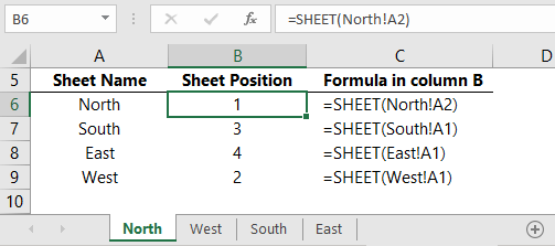
Use SHEET Function to Return a Sheet Index

Let’s say you have a list of your sheet names in column A and you want to find their position in the workbook. We can use the INDIRECT function to populate the ‘value’ argument by returning the sheet name from column A and appending it to cell reference A1, as shown below:

use SHEET function to return a sheet index

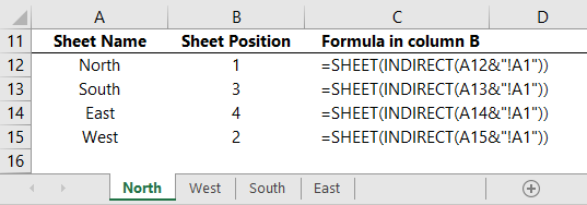
Sort Sheet Index with INDEX & MATCH Functions

We can then use INDEX & MATCH to return a sorted list of the sheets listed in cells A12:A15 based on their sheet position in cells B12:B15:

sort sheet index with INDEX & MATCH functions

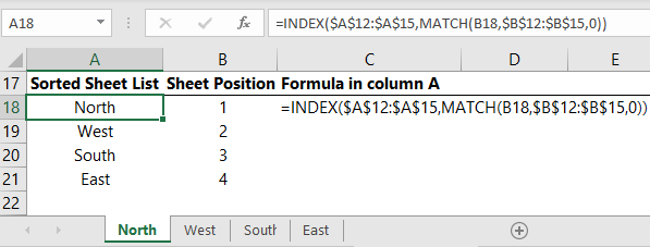
If any changes are made to the sheet order, the table above will automatically update.

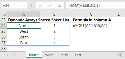
Sort Sheet Index with SORT Function

Or if you have Office 365 and the new Dynamic Array formulas you can use the SORT function:

sort sheet index with SORT function

Download the Excel Example File

Enter your email address below to download the sample workbook.

By submitting your email address you agree that we can email you our Excel newsletter.

Excel Sheet Function Related Lessons

Automatically generate a list of sheet names

Понравилась статья? Поделить с друзьями:
  • Sheet cell value excel
  • Short story one word answers
  • Short sentences with word many
  • Sheet add after excel
  • Short sentences with word like