Всё о работе с ячейками в Excel-VBA: обращение, перебор, удаление, вставка, скрытие, смена имени.
Содержание:
Table of Contents:
- Что такое ячейка Excel?
- Способы обращения к ячейкам
- Выбор и активация
- Получение и изменение значений ячеек
- Ячейки открытой книги
- Ячейки закрытой книги
- Перебор ячеек
- Перебор в произвольном диапазоне
- Свойства и методы ячеек
- Имя ячейки
- Адрес ячейки
- Размеры ячейки
- Запуск макроса активацией ячейки
2 нюанса:
- Я почти везде стараюсь использовать ThisWorkbook (а не, например, ActiveWorkbook) для обращения к текущей книге, в которой написан этот код (считаю это наиболее безопасным для новичков способом обращения к книгам, чтобы случайно не внести изменения в другие книги). Для экспериментов можете вставлять этот код в модули, коды книги, либо листа, и он будет работать только в пределах этой книги.
- Я использую английский эксель и у меня по стандарту листы называются Sheet1, Sheet2 и т.д. Если вы работаете в русском экселе, то замените Thisworkbook.Sheets(«Sheet1») на Thisworkbook.Sheets(«Лист1»). Если этого не сделать, то вы получите ошибку в связи с тем, что пытаетесь обратиться к несуществующему объекту. Можно также заменить на Thisworkbook.Sheets(1), но это менее безопасно.
Что такое ячейка Excel?
В большинстве мест пишут: «элемент, образованный пересечением столбца и строки». Это определение полезно для людей, которые не знакомы с понятием «таблица». Для того, чтобы понять чем на самом деле является ячейка Excel, необходимо заглянуть в объектную модель Excel. При этом определения объектов «ряд», «столбец» и «ячейка» будут отличаться в зависимости от того, как мы работаем с файлом.
Объекты в Excel-VBA. Пока мы работаем в Excel без углубления в VBA определение ячейки как «пересечения» строк и столбцов нам вполне хватает, но если мы решаем как-то автоматизировать процесс в VBA, то о нём лучше забыть и просто воспринимать лист как «мешок» ячеек, с каждой из которых VBA позволяет работать как минимум тремя способами:
- по цифровым координатам (ряд, столбец),
- по адресам формата А1, B2 и т.д. (сценарий целесообразности данного способа обращения в VBA мне сложно представить)
- по уникальному имени (во втором и третьем вариантах мы будем иметь дело не совсем с ячейкой, а с объектом VBA range, который может состоять из одной или нескольких ячеек). Функции и методы объектов Cells и Range отличаются. Новичкам я бы порекомендовал работать с ячейками VBA только с помощью Cells и по их цифровым координатам и использовать Range только по необходимости.
Все три способа обращения описаны далее
Как это хранится на диске и как с этим работать вне Excel? С точки зрения хранения и обработки вне Excel и VBA. Сделать это можно, например, сменив расширение файла с .xls(x) на .zip и открыв этот архив.
Пример содержимого файла Excel:
Далее xl -> worksheets и мы видим файл листа
Содержимое файла:
То же, но более наглядно:
<?xml version="1.0" encoding="UTF-8" standalone="yes"?>
<worksheet xmlns="http://schemas.openxmlformats.org/spreadsheetml/2006/main" xmlns:r="http://schemas.openxmlformats.org/officeDocument/2006/relationships" xmlns:mc="http://schemas.openxmlformats.org/markup-compatibility/2006" mc:Ignorable="x14ac xr xr2 xr3" xmlns:x14ac="http://schemas.microsoft.com/office/spreadsheetml/2009/9/ac" xmlns:xr="http://schemas.microsoft.com/office/spreadsheetml/2014/revision" xmlns:xr2="http://schemas.microsoft.com/office/spreadsheetml/2015/revision2" xmlns:xr3="http://schemas.microsoft.com/office/spreadsheetml/2016/revision3" xr:uid="{00000000-0001-0000-0000-000000000000}">
	<dimension ref="B2:F6"/>
	<sheetViews>
		<sheetView tabSelected="1" workbookViewId="0">
			<selection activeCell="D12" sqref="D12"/>
		</sheetView>
	</sheetViews>
	<sheetFormatPr defaultRowHeight="14.4" x14ac:dyDescent="0.3"/>
	<sheetData>
		<row r="2" spans="2:6" x14ac:dyDescent="0.3">
			<c r="B2" t="s">
				<v>0</v>
			</c>
		</row>
		<row r="3" spans="2:6" x14ac:dyDescent="0.3">
			<c r="C3" t="s">
				<v>1</v>
			</c>
		</row>
		<row r="4" spans="2:6" x14ac:dyDescent="0.3">
			<c r="D4" t="s">
				<v>2</v>
			</c>
		</row>
		<row r="5" spans="2:6" x14ac:dyDescent="0.3">
			<c r="E5" t="s">
				<v>0</v></c>
		</row>
		<row r="6" spans="2:6" x14ac:dyDescent="0.3">
			<c r="F6" t="s"><v>3</v>
		</c></row>
	</sheetData>
	<pageMargins left="0.7" right="0.7" top="0.75" bottom="0.75" header="0.3" footer="0.3"/>
</worksheet>
Как мы видим, в структуре объектной модели нет никаких «пересечений». Строго говоря рабочая книга — это архив структурированных данных в формате XML. При этом в каждую «строку» входит «столбец», и в нём в свою очередь прописан номер значения данного столбца, по которому оно подтягивается из другого XML файла при открытии книги для экономии места за счёт отсутствия повторяющихся значений. Почему это важно. Если мы захотим написать какой-то обработчик таких файлов, который будет напрямую редактировать данные в этих XML, то ориентироваться надо на такую модель и структуру данных. И правильное определение будет примерно таким: ячейка — это объект внутри столбца, который в свою очередь находится внутри строки в файле xml, в котором хранятся данные о содержимом листа.
Способы обращения к ячейкам
Выбор и активация
Почти во всех случаях можно и стоит избегать использования методов Select и Activate. На это есть две причины:
- Это лишь имитация действий пользователя, которая замедляет выполнение программы. Работать с объектами книги можно напрямую без использования методов Select и Activate.
- Это усложняет код и может приводить к неожиданным последствиям. Каждый раз перед использованием Select необходимо помнить, какие ещё объекты были выбраны до этого и не забывать при необходимости снимать выбор. Либо, например, в случае использования метода Select в самом начале программы может быть выбрано два листа вместо одного потому что пользователь запустил программу, выбрав другой лист.
Можно выбирать и активировать книги, листы, ячейки, фигуры, диаграммы, срезы, таблицы и т.д.
Отменить выбор ячеек можно методом Unselect:
Selection.UnselectОтличие выбора от активации — активировать можно только один объект из раннее выбранных. Выбрать можно несколько объектов.
Если вы записали и редактируете код макроса, то лучше всего заменить Select и Activate на конструкцию With … End With. Например, предположим, что мы записали вот такой макрос:
Sub Macro1()
' Macro1 Macro
    Range("F4:F10,H6:H10").Select 'выбрали два несмежных диапазона зажав ctrl
    Range("H6").Activate          'показывает только то, что я начал выбирать второй диапазон с этой ячейки (она осталась белой). Это действие ни на что не влияет
    With Selection.Interior
        .Pattern = xlSolid
        .PatternColorIndex = xlAutomatic
        .Color = 65535            'залили желтым цветом, нажав на кнопку заливки на верхней панели
        .TintAndShade = 0
        .PatternTintAndShade = 0
    End With
End Sub
Почему макрос записался таким неэффективным образом? Потому что в каждый момент времени (в каждой строке) программа не знает, что вы будете делать дальше. Поэтому в записи выбор ячеек и действия с ними — это два отдельных действия. Этот код лучше всего оптимизировать (особенно если вы хотите скопировать его внутрь какого-нибудь цикла, который должен будет исполняться много раз и перебирать много объектов). Например, так:
Sub Macro11()
'
' Macro1 Macro
    Range("F4:F10,H6:H10").Select '1. смотрим, что за объект выбран (что идёт до .Select)
    Range("H6").Activate
    With Selection.Interior       '2. понимаем, что у выбранного объекта есть свойство interior, с которым далее идёт работа
        .Pattern = xlSolid
        .PatternColorIndex = xlAutomatic
        .Color = 65535
        .TintAndShade = 0
        .PatternTintAndShade = 0
    End With
End Sub


Sub Optimized_Macro()
    With Range("F4:F10,H6:H10").Interior '3. переносим объект напрямую в конструкцию With вместо Selection
' ////// Здесь я для надёжности прописал бы ещё Thisworkbook.Sheet("ИмяЛиста") перед Range,
' ////// чтобы минимизировать риск любых случайных изменений других листов и книг
' ////// With Thisworkbook.Sheet("ИмяЛиста").Range("F4:F10,H6:H10").Interior
        .Pattern = xlSolid               '4. полностью копируем всё, что было записано рекордером внутрь блока with
        .PatternColorIndex = xlAutomatic
        .Color = 55555                   '5. здесь я поменял цвет на зеленый, чтобы было видно, работает ли код при поочерёдном запуске двух макросов
        .TintAndShade = 0
        .PatternTintAndShade = 0
    End With
End Sub
Пример сценария, когда использование Select и Activate оправдано:
Допустим, мы хотим, чтобы во время исполнения программы мы одновременно изменяли несколько листов одним действием и пользователь видел какой-то определённый лист. Это можно сделать примерно так:
Sub Select_Activate_is_OK()
Thisworkbook.Worksheets(Array("Sheet1", "Sheet3")).Select 'Выбираем несколько листов по именам
Thisworkbook.Worksheets("Sheet3").Activate 'Показываем пользователю третий лист
'Далее все действия с выбранными ячейками через Select будут одновременно вносить изменения в оба выбранных листа

'Допустим, что тут мы решили покрасить те же два диапазона:
Range("F4:F10,H6:H10").Select
    Range("H6").Activate
    With Selection.Interior
        .Pattern = xlSolid
        .PatternColorIndex = xlAutomatic
        .Color = 65535
        .TintAndShade = 0
        .PatternTintAndShade = 0
    End With

End Sub
Единственной причиной использовать этот код по моему мнению может быть желание зачем-то показать пользователю определённую страницу книги в какой-то момент исполнения программы. С точки зрения обработки объектов, опять же, эти действия лишние.
Получение и изменение значений ячеек
Значение ячеек можно получать/изменять с помощью свойства value.
'Если нужно прочитать / записать значение ячейки, то используется свойство Value
a = ThisWorkbook.Sheets("Sheet1").Cells (1,1).Value 'записать значение ячейки А1 листа "Sheet1" в переменную "a"
ThisWorkbook.Sheets("Sheet1").Cells (1,1).Value = 1  'задать значение ячейки А1 (первый ряд, первый столбец) листа "Sheet1"

'Если нужно прочитать текст как есть (с форматированием), то можно использовать свойство .text:
ThisWorkbook.Sheets("Sheet1").Cells (1,1).Text = "1"
a = ThisWorkbook.Sheets("Sheet1").Cells (1,1).Text

'Когда проявится разница:
'Например, если мы считываем дату в формате "31 декабря 2021 г.", хранящуюся как дата
a = ThisWorkbook.Sheets("Sheet1").Cells (1,1).Value 'эапишет как "31.12.2021"
a = ThisWorkbook.Sheets("Sheet1").Cells (1,1).Text  'запишет как "31 декабря 2021 г."
Ячейки открытой книги
К ячейкам можно обращаться:
'В книге, в которой хранится макрос (на каком-то из листов, либо в отдельном модуле или форме)
ThisWorkbook.Sheets("Sheet1").Cells(1,1).Value        'По номерам строки и столбца
ThisWorkbook.Sheets("Sheet1").Cells(1,"A").Value      'По номерам строки и букве столбца
ThisWorkbook.Sheets("Sheet1").Range("A1").Value       'По адресу - вариант 1
ThisWorkbook.Sheets("Sheet1").[A1].Value              'По адресу - вариант 2
ThisWorkbook.Sheets("Sheet1").Range("CellName").Value 'По имени ячейки (для этого ей предварительно нужно его присвоить)

'Те же действия, но с использованием полного названия рабочей книги (книга должна быть открыта)
Workbooks("workbook.xlsm").Sheets("Sheet1").Cells(1,1).Value 'По номерам строки и столбца
Workbooks("workbook.xlsm").Sheets("Sheet1").Cells(1,"A").Value                'По номерам строки и букве столбца
Workbooks("workbook.xlsm").Sheets("Sheet1").Range("A1").Value                 'По адресу - вариант 1
Workbooks("workbook.xlsm").Sheets("Sheet1").[A1].Value                        'По адресу - вариант 2
Workbooks("workbook.xlsm").Sheets("Sheet1").Range("CellName").Value           'По имени ячейки (для этого ей предварительно нужно его присвоить)
Ячейки закрытой книги
Если нужно достать или изменить данные в другой закрытой книге, то необходимо прописать открытие и закрытие книги. Непосредственно работать с закрытой книгой не получится, потому что данные в ней хранятся отдельно от структуры и при открытии Excel каждый раз производит расстановку значений по соответствующим «слотам» в структуре. Подробнее о том, как хранятся данные в xlsx см выше.
Workbooks.Open Filename:="С:closed_workbook.xlsx"    'открыть книгу (она становится активной)
a = ActiveWorkbook.Sheets("Sheet1").Cells(1,1).Value  'достать значение ячейки 1,1
ActiveWorkbook.Close False                            'закрыть книгу (False => без сохранения)
Скачать пример, в котором можно посмотреть, как доставать и как записывать значения в закрытую книгу.
Код из файла:
Option Explicit
Sub get_value_from_closed_wb() 'достать значение из закрытой книги
Dim a, wb_path, wsh As String
wb_path = ThisWorkbook.Sheets("Sheet1").Cells(2, 3).Value 'get path to workbook from sheet1
wsh = ThisWorkbook.Sheets("Sheet1").Cells(3, 3).Value
Workbooks.Open Filename:=wb_path
a = ActiveWorkbook.Sheets(wsh).Cells(3, 3).Value
ActiveWorkbook.Close False
ThisWorkbook.Sheets("Sheet1").Cells(4, 3).Value = a
End Sub

Sub record_value_to_closed_wb() 'записать значение в закрытую книгу
Dim wb_path, b, wsh As String
wsh = ThisWorkbook.Sheets("Sheet1").Cells(3, 3).Value
wb_path = ThisWorkbook.Sheets("Sheet1").Cells(2, 3).Value 'get path to workbook from sheet1
b = ThisWorkbook.Sheets("Sheet1").Cells(5, 3).Value 'get value to record in the target workbook
Workbooks.Open Filename:=wb_path
ActiveWorkbook.Sheets(wsh).Cells(4, 4).Value = b 'add new value to cell D4 of the target workbook
ActiveWorkbook.Close True
End Sub
Перебор ячеек
Перебор в произвольном диапазоне
Скачать файл со всеми примерами
Пройтись по всем ячейкам в нужном диапазоне можно разными способами. Основные:
- Цикл For Each. Пример:
Sub iterate_over_cells() For Each c In ThisWorkbook.Sheets("Sheet1").Range("B2:D4").Cells MsgBox (c) Next c End SubЭтот цикл выведет в виде сообщений значения ячеек в диапазоне B2:D4 по порядку по строкам слева направо и по столбцам — сверху вниз. Данный способ можно использовать для действий, в который вам не важны номера ячеек (закрашивание, изменение форматирования, пересчёт чего-то и т.д.).
- Ту же задачу можно решить с помощью двух вложенных циклов — внешний будет перебирать ряды, а вложенный — ячейки в рядах. Этот способ я использую чаще всего, потому что он позволяет получить больше контроля над исполнением: на каждой итерации цикла нам доступны координаты ячеек. Для перебора всех ячеек на листе этим методом потребуется найти последнюю заполненную ячейку. Пример кода:
Sub iterate_over_cells() Dim cl, rw As Integer Dim x As Variant 'перебор области 3x3 For rw = 1 To 3 ' цикл для перебора рядов 1-3 For cl = 1 To 3 'цикл для перебора столбцов 1-3 x = ThisWorkbook.Sheets("Sheet1").Cells(rw + 1, cl + 1).Value MsgBox (x) Next cl Next rw 'перебор всех ячеек на листе. Последняя ячейка определена с помощью UsedRange 'LastRow = ActiveSheet.UsedRange.Row + ActiveSheet.UsedRange.Rows.Count - 1 'LastCol = ActiveSheet.UsedRange.Column + ActiveSheet.UsedRange.Columns.Count - 1 'For rw = 1 To LastRow 'цикл перебора всех рядов ' For cl = 1 To LastCol 'цикл для перебора всех столбцов ' Действия ' Next cl 'Next rw End Sub - Если нужно перебрать все ячейки в выделенном диапазоне на активном листе, то код будет выглядеть так:
Sub iterate_cell_by_cell_over_selection() Dim ActSheet As Worksheet Dim SelRange As Range Dim cell As Range Set ActSheet = ActiveSheet Set SelRange = Selection 'if we want to do it in every cell of the selected range For Each cell In Selection MsgBox (cell.Value) Next cell End SubДанный метод подходит для интерактивных макросов, которые выполняют действия над выбранными пользователем областями.
- Перебор ячеек в ряду
Sub iterate_cells_in_row() Dim i, RowNum, StartCell As Long RowNum = 3 'какой ряд StartCell = 0 ' номер начальной ячейки (минус 1, т.к. в цикле мы прибавляем i) For i = 1 To 10 ' 10 ячеек в выбранном ряду ThisWorkbook.Sheets("Sheet1").Cells(RowNum, i + StartCell).Value = i '(i + StartCell) добавляет 1 к номеру столбца при каждом повторении Next i End Sub - Перебор ячеек в столбце
Sub iterate_cells_in_column() Dim i, ColNum, StartCell As Long ColNum = 3 'какой столбец StartCell = 0 ' номер начальной ячейки (минус 1, т.к. в цикле мы прибавляем i) For i = 1 To 10 ' 10 ячеек ThisWorkbook.Sheets("Sheet1").Cells(i + StartCell, ColNum).Value = i ' (i + StartCell) добавляет 1 к номеру ряда при каждом повторении Next i End Sub
Свойства и методы ячеек
Имя ячейки
Присвоить новое имя можно так:
Thisworkbook.Sheets(1).Cells(1,1).name = "Новое_Имя"Для того, чтобы сменить имя ячейки нужно сначала удалить существующее имя, а затем присвоить новое. Удалить имя можно так:
ActiveWorkbook.Names("Старое_Имя").DeleteПример кода для переименования ячеек:
Sub rename_cell()

old_name = "Cell_Old_Name"
new_name = "Cell_New_Name"

ActiveWorkbook.Names(old_name).Delete
ThisWorkbook.Sheets(1).Cells(2, 1).Name = new_name
End Sub

Sub rename_cell_reverse()

old_name = "Cell_New_Name"
new_name = "Cell_Old_Name"

ActiveWorkbook.Names(old_name).Delete
ThisWorkbook.Sheets(1).Cells(2, 1).Name = new_name
End Sub
Адрес ячейки
Sub get_cell_address() ' вывести адрес ячейки в формате буква столбца, номер ряда
  '$A$1 style
  txt_address = ThisWorkbook.Sheets(1).Cells(3, 2).Address
  MsgBox (txt_address)
End Sub

Sub get_cell_address_R1C1()' получить адрес столбца в формате номер ряда, номер столбца
  'R1C1 style
  txt_address = ThisWorkbook.Sheets(1).Cells(3, 2).Address(ReferenceStyle:=xlR1C1)
  MsgBox (txt_address)
End Sub

  'пример функции, которая принимает 2 аргумента: название именованного диапазона и тип желаемого адреса
  '(1- тип $A$1 2- R1C1 - номер ряда, столбца)
Function get_cell_address_by_name(str As String, address_type As Integer)
  '$A$1 style
  Select Case address_type
    Case 1
      txt_address = Range(str).Address
    Case 2
      txt_address = Range(str).Address(ReferenceStyle:=xlR1C1)
    Case Else
      txt_address = "Wrong address type selected. 1,2 available"
    End Select
  get_cell_address_by_name = txt_address
End Function

'перед запуском нужно убедиться, что в книге есть диапазон с названием,
'адрес которого мы хотим получить, иначе будет ошибка
Sub test_function() 'запустите эту программу, чтобы увидеть, как работает функция
  x = get_cell_address_by_name("MyValue", 2)
  MsgBox (x)
End Sub
Размеры ячейки
Ширина и длина ячейки в VBA меняется, например, так:
Sub change_size()
Dim x, y As Integer
Dim w, h As Double

'получить координаты целевой ячейки
x = ThisWorkbook.Sheets("Sheet1").Cells(2, 2).Value
y = ThisWorkbook.Sheets("Sheet1").Cells(3, 2).Value

'получить желаемую ширину и высоту ячейки
w = ThisWorkbook.Sheets("Sheet1").Cells(6, 2).Value
h = ThisWorkbook.Sheets("Sheet1").Cells(7, 2).Value

'сменить высоту и ширину ячейки с координатами x,y
ThisWorkbook.Sheets("Sheet1").Cells(x, y).RowHeight = h
ThisWorkbook.Sheets("Sheet1").Cells(x, y).ColumnWidth = w


End Sub
Прочитать значения ширины и высоты ячеек можно двумя способами (однако результаты будут в разных единицах измерения). Если написать просто Cells(x,y).Width или Cells(x,y).Height, то будет получен результат в pt (привязка к размеру шрифта).
Sub get_size()
Dim x, y As Integer
'получить координаты ячейки, с которой мы будем работать
x = ThisWorkbook.Sheets("Sheet1").Cells(2, 2).Value
y = ThisWorkbook.Sheets("Sheet1").Cells(3, 2).Value

'получить длину и ширину выбранной ячейки в тех же единицах измерения, в которых мы их задавали
ThisWorkbook.Sheets("Sheet1").Cells(2, 6).Value = ThisWorkbook.Sheets("Sheet1").Cells(x, y).ColumnWidth
ThisWorkbook.Sheets("Sheet1").Cells(3, 6).Value = ThisWorkbook.Sheets("Sheet1").Cells(x, y).RowHeight

'получить длину и ширину с помощью свойств ячейки (только для чтения) в поинтах (pt)
ThisWorkbook.Sheets("Sheet1").Cells(7, 9).Value = ThisWorkbook.Sheets("Sheet1").Cells(x, y).Width
ThisWorkbook.Sheets("Sheet1").Cells(8, 9).Value = ThisWorkbook.Sheets("Sheet1").Cells(x, y).Height

End Sub
Скачать файл с примерами изменения и чтения размера ячеек
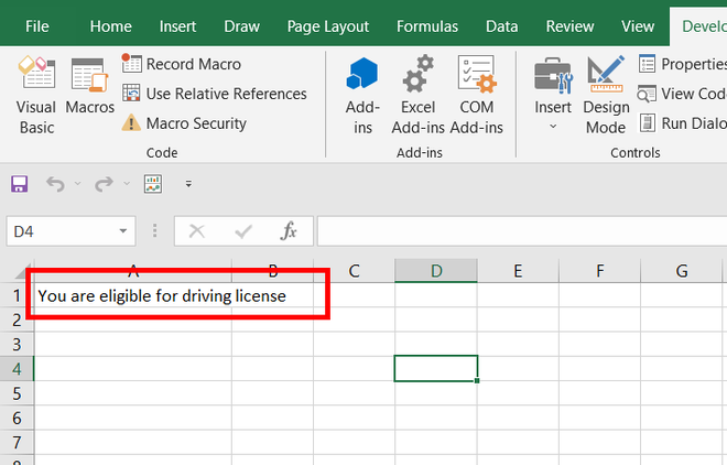
Запуск макроса активацией ячейки
Для запуска кода VBA при активации ячейки необходимо вставить в код листа нечто подобное:
3 важных момента, чтобы это работало:
1. Этот код должен быть вставлен в код листа (здесь контролируется диапазон D4)
2-3. Программа, ответственная за запуск кода при выборе ячейки, должна называться Worksheet_SelectionChange и должна принимать значение переменной Target, относящейся к триггеру SelectionChange. Другие доступные триггеры можно посмотреть в правом верхнем углу (2).
Скачать файл с базовым примером (как на картинке)
Скачать файл с расширенным примером (код ниже)
Option Explicit

Private Sub Worksheet_SelectionChange(ByVal Target As Range)

        ' имеем в виду, что триггер SelectionChange будет запускать эту Sub после каждого клика мышью (после каждого клика будет проверяться:
          '1. количество выделенных ячеек и
          '2. не пересекается ли выбранный диапазон с заданным в этой программе диапазоном.
        ' поэтому в эту программу не стоит без необходимости писать никаких других тяжелых операций

    If Selection.Count = 1 Then 'запускаем программу только если выбрано не более 1 ячейки


    'вариант модификации - брать адрес ячейки из другой ячейки:
    'Dim CellName as String
    'CellName = Activesheet.Cells(1,1).value 'брать текстовое имя контролируемой ячейки из A1 (должно быть в формате Буква столбца + номер строки)
    'If Not Intersect(Range(CellName), Target) Is Nothing Then
    'для работы этой модификации следующую строку надо закомментировать/удалить


        If Not Intersect(Range("D4"), Target) Is Nothing Then
        'если заданный (D4) и выбранный диапазон пересекаются
        '(пересечение диапазонов НЕ равно Nothing)

        'можно прописать диапазон из нескольких ячеек:
        'If Not Intersect(Range("D4:E10"), Target) Is Nothing Then
        'можно прописать несколько диапазонов:
        'If Not Intersect(Range("D4:E10"), Target) Is Nothing or Not Intersect(Range("A4:A10"), Target) Is Nothing Then

            Call program 'выполняем программу
        End If
    End If
End Sub

Sub program()

MsgBox ("Program Is running") 'здесь пишем код того, что произойдёт при выборе нужной ячейки


End Sub
На чтение 18 мин. Просмотров 75.1k.

сэр Артур Конан Дойл
Это большая ошибка — теоретизировать, прежде чем кто-то получит данные
Эта статья охватывает все, что вам нужно знать об использовании ячеек и диапазонов в VBA. Вы можете прочитать его от начала до конца, так как он сложен в логическом порядке. Или использовать оглавление ниже, чтобы перейти к разделу по вашему выбору.
Рассматриваемые темы включают свойство смещения, чтение
значений между ячейками, чтение значений в массивы и форматирование ячеек.
Содержание
- Краткое руководство по диапазонам и клеткам
- Введение
- Важное замечание
- Свойство Range
- Свойство Cells рабочего листа
- Использование Cells и Range вместе
- Свойство Offset диапазона
- Использование диапазона CurrentRegion
- Использование Rows и Columns в качестве Ranges
- Использование Range вместо Worksheet
- Чтение значений из одной ячейки в другую
- Использование метода Range.Resize
- Чтение Value в переменные
- Как копировать и вставлять ячейки
- Чтение диапазона ячеек в массив
- Пройти через все клетки в диапазоне
- Форматирование ячеек
- Основные моменты
Краткое руководство по диапазонам и клеткам
| Функция | Принимает | Возвращает | Пример | Вид |
| Range | адреса ячеек |
диапазон ячеек |
.Range(«A1:A4») | $A$1:$A$4 |
| Cells | строка, столбец |
одна ячейка |
.Cells(1,5) | $E$1 |
| Offset | строка, столбец |
диапазон | .Range(«A1:A2») .Offset(1,2) |
$C$2:$C$3 |
| Rows | строка (-и) | одна или несколько строк |
.Rows(4) .Rows(«2:4») |
$4:$4 $2:$4 |
| Columns | столбец (-цы) |
один или несколько столбцов |
.Columns(4) .Columns(«B:D») |
$D:$D $B:$D |
Введение
Это третья статья, посвященная трем основным элементам VBA. Этими тремя элементами являются Workbooks, Worksheets и Ranges/Cells. Cells, безусловно, самая важная часть Excel. Почти все, что вы делаете в Excel, начинается и заканчивается ячейками.
Вы делаете три основных вещи с помощью ячеек:
- Читаете из ячейки.
- Пишите в ячейку.
- Изменяете формат ячейки.
В Excel есть несколько методов для доступа к ячейкам, таких как Range, Cells и Offset. Можно запутаться, так как эти функции делают похожие операции.
В этой статье я расскажу о каждом из них, объясню, почему они вам нужны, и когда вам следует их использовать.
Давайте начнем с самого простого метода доступа к ячейкам — с помощью свойства Range рабочего листа.
Важное замечание
Я недавно обновил эту статью, сейчас использую Value2.
Вам может быть интересно, в чем разница между Value, Value2 и значением по умолчанию:
' Value2
Range("A1").Value2 = 56

' Value
Range("A1").Value = 56

' По умолчанию используется значение
Range("A1") = 56
Использование Value может усечь число, если ячейка отформатирована, как валюта. Если вы не используете какое-либо свойство, по умолчанию используется Value.
Лучше использовать Value2, поскольку он всегда будет возвращать фактическое значение ячейки.
Свойство Range
Рабочий лист имеет свойство Range, которое можно использовать для доступа к ячейкам в VBA. Свойство Range принимает тот же аргумент, что и большинство функций Excel Worksheet, например: «А1», «А3: С6» и т.д.
В следующем примере показано, как поместить значение в ячейку с помощью свойства Range.
Sub ZapisVYacheiku()

    ' Запишите число в ячейку A1 на листе 1 этой книги
    ThisWorkbook.Worksheets("Лист1").Range("A1").Value2 = 67

    ' Напишите текст в ячейку A2 на листе 1 этой рабочей книги
    ThisWorkbook.Worksheets("Лист1").Range("A2").Value2 = "Иван Петров"

    ' Запишите дату в ячейку A3 на листе 1 этой книги
    ThisWorkbook.Worksheets("Лист1").Range("A3").Value2 = #11/21/2019#

End Sub
Как видно из кода, Range является членом Worksheets, которая, в свою очередь, является членом Workbook. Иерархия такая же, как и в Excel, поэтому должно быть легко понять. Чтобы сделать что-то с Range, вы должны сначала указать рабочую книгу и рабочий лист, которому она принадлежит.
В оставшейся части этой статьи я буду использовать кодовое имя для ссылки на лист.

Следующий код показывает приведенный выше пример с использованием кодового имени рабочего листа, т.е. Лист1 вместо ThisWorkbook.Worksheets («Лист1»).
Sub IspKodImya ()

    ' Запишите число в ячейку A1 на листе 1 этой книги
     Sheet1.Range("A1").Value2 = 67

    ' Напишите текст в ячейку A2 на листе 1 этой рабочей книги
    Sheet1.Range("A2").Value2 = "Иван Петров"

    ' Запишите дату в ячейку A3 на листе 1 этой книги
    Sheet1.Range("A3").Value2 = #11/21/2019#

End Sub
Вы также можете писать в несколько ячеек, используя свойство
Range
Sub ZapisNeskol()

    ' Запишите число в диапазон ячеек
    Sheet1.Range("A1:A10").Value2 = 67

    ' Написать текст в несколько диапазонов ячеек
    Sheet1.Range("B2:B5,B7:B9").Value2 = "Иван Петров"

End Sub
Свойство Cells рабочего листа
У Объекта листа есть другое свойство, называемое Cells, которое очень похоже на Range . Есть два отличия:
- Cells возвращают диапазон только одной ячейки.
- Cells принимает строку и столбец в качестве аргументов.
В приведенном ниже примере показано, как записывать значения
в ячейки, используя свойства Range и Cells.
Sub IspCells()

    ' Написать в А1
    Sheet1.Range("A1").Value2 = 10
    Sheet1.Cells(1, 1).Value2  = 10

    ' Написать в А10
    Sheet1.Range("A10").Value2 = 10
    Sheet1.Cells(10, 1).Value2  = 10

    ' Написать в E1
    Sheet1.Range("E1").Value2 = 10
    Sheet1.Cells(1, 5).Value2  = 10

End Sub
Вам должно быть интересно, когда использовать Cells, а когда Range. Использование Range полезно для доступа к одним и тем же ячейкам при каждом запуске макроса.
Например, если вы использовали макрос для вычисления суммы и
каждый раз записывали ее в ячейку A10, тогда Range подойдет для этой задачи.
Использование свойства Cells полезно, если вы обращаетесь к
ячейке по номеру, который может отличаться. Проще объяснить это на примере.
В следующем коде мы просим пользователя указать номер столбца. Использование Cells дает нам возможность использовать переменное число для столбца.
Sub ZapisVPervuyuPustuyuYacheiku()

    Dim UserCol As Integer

    ' Получить номер столбца от пользователя
    UserCol = Application.InputBox("Пожалуйста, введите номер столбца...", Type:=1)

    ' Написать текст в выбранный пользователем столбец
    Sheet1.Cells(1, UserCol).Value2 = "Иван Петров"

End Sub
В приведенном выше примере мы используем номер для столбца,
а не букву.
Чтобы использовать Range здесь, потребуется преобразовать эти значения в ссылку на
буквенно-цифровую ячейку, например, «С1». Использование свойства Cells позволяет нам
предоставить строку и номер столбца для доступа к ячейке.
Иногда вам может понадобиться вернуть более одной ячейки, используя номера строк и столбцов. В следующем разделе показано, как это сделать.
Использование Cells и Range вместе
Как вы уже видели, вы можете получить доступ только к одной ячейке, используя свойство Cells. Если вы хотите вернуть диапазон ячеек, вы можете использовать Cells с Range следующим образом:
Sub IspCellsSRange()

    With Sheet1
        ' Запишите 5 в диапазон A1: A10, используя свойство Cells
        .Range(.Cells(1, 1), .Cells(10, 1)).Value2 = 5

        ' Диапазон B1: Z1 будет выделен жирным шрифтом
        .Range(.Cells(1, 2), .Cells(1, 26)).Font.Bold = True

    End With

End Sub
Как видите, вы предоставляете начальную и конечную ячейку
диапазона. Иногда бывает сложно увидеть, с каким диапазоном вы имеете дело,
когда значением являются все числа. Range имеет свойство Address, которое
отображает буквенно-цифровую ячейку для любого диапазона. Это может
пригодиться, когда вы впервые отлаживаете или пишете код.
В следующем примере мы распечатываем адрес используемых нами
диапазонов.
Sub PokazatAdresDiapazona()

    ' Примечание. Использование подчеркивания позволяет разделить строки кода.
    With Sheet1

        ' Запишите 5 в диапазон A1: A10, используя свойство Cells
        .Range(.Cells(1, 1), .Cells(10, 1)).Value2 = 5
        Debug.Print "Первый адрес: " _
            + .Range(.Cells(1, 1), .Cells(10, 1)).Address

        ' Диапазон B1: Z1 будет выделен жирным шрифтом
        .Range(.Cells(1, 2), .Cells(1, 26)).Font.Bold = True
        Debug.Print "Второй адрес : " _
            + .Range(.Cells(1, 2), .Cells(1, 26)).Address

    End With

End Sub
В примере я использовал Debug.Print для печати в Immediate Window. Для просмотра этого окна выберите «View» -> «в Immediate Window» (Ctrl + G).


Свойство Offset диапазона
У диапазона есть свойство, которое называется Offset. Термин «Offset» относится к отсчету от исходной позиции. Он часто используется в определенных областях программирования. С помощью свойства «Offset» вы можете получить диапазон ячеек того же размера и на определенном расстоянии от текущего диапазона. Это полезно, потому что иногда вы можете выбрать диапазон на основе определенного условия. Например, на скриншоте ниже есть столбец для каждого дня недели. Учитывая номер дня (т.е. понедельник = 1, вторник = 2 и т.д.). Нам нужно записать значение в правильный столбец.

Сначала мы попытаемся сделать это без использования Offset.
' Это Sub тесты с разными значениями
Sub TestSelect()

    ' Понедельник
    SetValueSelect 1, 111.21
    ' Среда
    SetValueSelect 3, 456.99
    ' Пятница
    SetValueSelect 5, 432.25
    ' Воскресение
    SetValueSelect 7, 710.17

End Sub

' Записывает значение в столбец на основе дня
Public Sub SetValueSelect(lDay As Long, lValue As Currency)

    Select Case lDay
        Case 1: Sheet1.Range("H3").Value2 = lValue
        Case 2: Sheet1.Range("I3").Value2 = lValue
        Case 3: Sheet1.Range("J3").Value2 = lValue
        Case 4: Sheet1.Range("K3").Value2 = lValue
        Case 5: Sheet1.Range("L3").Value2 = lValue
        Case 6: Sheet1.Range("M3").Value2 = lValue
        Case 7: Sheet1.Range("N3").Value2 = lValue
    End Select

End Sub
Как видно из примера, нам нужно добавить строку для каждого возможного варианта. Это не идеальная ситуация. Использование свойства Offset обеспечивает более чистое решение.
' Это Sub тесты с разными значениями
Sub TestOffset()

    DayOffSet 1, 111.01
    DayOffSet 3, 456.99
    DayOffSet 5, 432.25
    DayOffSet 7, 710.17

End Sub

Public Sub DayOffSet(lDay As Long, lValue As Currency)

    ' Мы используем значение дня с Offset, чтобы указать правильный столбец
    Sheet1.Range("G3").Offset(, lDay).Value2 = lValue

End Sub
Как видите, это решение намного лучше. Если количество дней увеличилось, нам больше не нужно добавлять код. Чтобы Offset был полезен, должна быть какая-то связь между позициями ячеек. Если столбцы Day в приведенном выше примере были случайными, мы не могли бы использовать Offset. Мы должны были бы использовать первое решение.
Следует иметь в виду, что Offset сохраняет размер диапазона. Итак .Range («A1:A3»).Offset (1,1) возвращает диапазон B2:B4. Ниже приведены еще несколько примеров использования Offset.
Sub IspOffset()

    ' Запись в В2 - без Offset
    Sheet1.Range("B2").Offset().Value2 = "Ячейка B2"

    ' Написать в C2 - 1 столбец справа
    Sheet1.Range("B2").Offset(, 1).Value2 = "Ячейка C2"

    ' Написать в B3 - 1 строка вниз
    Sheet1.Range("B2").Offset(1).Value2 = "Ячейка B3"

    ' Запись в C3 - 1 столбец справа и 1 строка вниз
    Sheet1.Range("B2").Offset(1, 1).Value2 = "Ячейка C3"

    ' Написать в A1 - 1 столбец слева и 1 строка вверх
    Sheet1.Range("B2").Offset(-1, -1).Value2 = "Ячейка A1"

    ' Запись в диапазон E3: G13 - 1 столбец справа и 1 строка вниз
    Sheet1.Range("D2:F12").Offset(1, 1).Value2 = "Ячейки E3:G13"

End Sub
Использование диапазона CurrentRegion
CurrentRegion возвращает диапазон всех соседних ячеек в данный диапазон. На скриншоте ниже вы можете увидеть два CurrentRegion. Я добавил границы, чтобы прояснить CurrentRegion.

Строка или столбец пустых ячеек означает конец CurrentRegion.
Вы можете вручную проверить
CurrentRegion в Excel, выбрав диапазон и нажав Ctrl + Shift + *.
Если мы возьмем любой диапазон
ячеек в пределах границы и применим CurrentRegion, мы вернем диапазон ячеек во
всей области.
Например:
Range («B3»). CurrentRegion вернет диапазон B3:D14
Range («D14»). CurrentRegion вернет диапазон B3:D14
Range («C8:C9»). CurrentRegion вернет диапазон B3:D14 и так далее
Как пользоваться
Мы получаем CurrentRegion следующим образом
' CurrentRegion вернет B3:D14 из приведенного выше примера
Dim rg As Range
Set rg = Sheet1.Range("B3").CurrentRegion
Только чтение строк данных
Прочитать диапазон из второй строки, т.е. пропустить строку заголовка.
' CurrentRegion вернет B3:D14 из приведенного выше примера
Dim rg As Range
Set rg = Sheet1.Range("B3").CurrentRegion

' Начало в строке 2 - строка после заголовка
Dim i As Long
For i = 2 To rg.Rows.Count
    ' текущая строка, столбец 1 диапазона
    Debug.Print rg.Cells(i, 1).Value2
Next i
Удалить заголовок
Удалить строку заголовка (т.е. первую строку) из диапазона. Например, если диапазон — A1:D4, это возвратит A2:D4
' CurrentRegion вернет B3:D14 из приведенного выше примера
Dim rg As Range
Set rg = Sheet1.Range("B3").CurrentRegion

' Удалить заголовок
Set rg = rg.Resize(rg.Rows.Count - 1).Offset(1)

' Начните со строки 1, так как нет строки заголовка
Dim i As Long
For i = 1 To rg.Rows.Count
    ' текущая строка, столбец 1 диапазона
    Debug.Print rg.Cells(i, 1).Value2
Next i
Использование Rows и Columns в качестве Ranges
Если вы хотите что-то сделать со всей строкой или столбцом,
вы можете использовать свойство «Rows и
Columns» на рабочем листе. Они оба принимают один параметр — номер строки
или столбца, к которому вы хотите получить доступ.
Sub IspRowIColumns()

    ' Установите размер шрифта столбца B на 9
    Sheet1.Columns(2).Font.Size = 9

    ' Установите ширину столбцов от D до F
    Sheet1.Columns("D:F").ColumnWidth = 4

    ' Установите размер шрифта строки 5 до 18
    Sheet1.Rows(5).Font.Size = 18

End Sub
Использование Range вместо Worksheet
Вы также можете использовать Cella, Rows и Columns, как часть Range, а не как часть Worksheet. У вас может быть особая необходимость в этом, но в противном случае я бы избегал практики. Это делает код более сложным. Простой код — твой друг. Это уменьшает вероятность ошибок.
Код ниже выделит второй столбец диапазона полужирным. Поскольку диапазон имеет только две строки, весь столбец считается B1:B2
Sub IspColumnsVRange()

    ' Это выделит B1 и B2 жирным шрифтом.
    Sheet1.Range("A1:C2").Columns(2).Font.Bold = True

End Sub
Чтение значений из одной ячейки в другую
В большинстве примеров мы записали значения в ячейку. Мы
делаем это, помещая диапазон слева от знака равенства и значение для размещения
в ячейке справа. Для записи данных из одной ячейки в другую мы делаем то же
самое. Диапазон назначения идет слева, а диапазон источника — справа.
В следующем примере показано, как это сделать:
Sub ChitatZnacheniya()

    ' Поместите значение из B1 в A1
    Sheet1.Range("A1").Value2 = Sheet1.Range("B1").Value2

    ' Поместите значение из B3 в лист2 в ячейку A1
    Sheet1.Range("A1").Value2 = Sheet2.Range("B3").Value2

    ' Поместите значение от B1 в ячейки A1 до A5
    Sheet1.Range("A1:A5").Value2 = Sheet1.Range("B1").Value2

    ' Вам необходимо использовать свойство «Value», чтобы прочитать несколько ячеек
    Sheet1.Range("A1:A5").Value2 = Sheet1.Range("B1:B5").Value2

End Sub
Как видно из этого примера, невозможно читать из нескольких ячеек. Если вы хотите сделать это, вы можете использовать функцию копирования Range с параметром Destination.
Sub KopirovatZnacheniya()

    ' Сохранить диапазон копирования в переменной
    Dim rgCopy As Range
    Set rgCopy = Sheet1.Range("B1:B5")

    ' Используйте это для копирования из более чем одной ячейки
    rgCopy.Copy Destination:=Sheet1.Range("A1:A5")

    ' Вы можете вставить в несколько мест назначения
    rgCopy.Copy Destination:=Sheet1.Range("A1:A5,C2:C6")

End Sub
Функция Copy копирует все, включая формат ячеек. Это тот же результат, что и ручное копирование и вставка выделения. Подробнее об этом вы можете узнать в разделе «Копирование и вставка ячеек»
Использование метода Range.Resize
При копировании из одного диапазона в другой с использованием присваивания (т.е. знака равенства) диапазон назначения должен быть того же размера, что и исходный диапазон.
Использование функции Resize позволяет изменить размер
диапазона до заданного количества строк и столбцов.
Например:
Sub ResizePrimeri()

    ' Печатает А1
    Debug.Print Sheet1.Range("A1").Address

    ' Печатает A1:A2
    Debug.Print Sheet1.Range("A1").Resize(2, 1).Address

    ' Печатает A1:A5
    Debug.Print Sheet1.Range("A1").Resize(5, 1).Address

    ' Печатает A1:D1
    Debug.Print Sheet1.Range("A1").Resize(1, 4).Address

    ' Печатает A1:C3
    Debug.Print Sheet1.Range("A1").Resize(3, 3).Address

End Sub
Когда мы хотим изменить наш целевой диапазон, мы можем
просто использовать исходный размер диапазона.
Другими словами, мы используем количество строк и столбцов
исходного диапазона в качестве параметров для изменения размера:
Sub Resize()

    Dim rgSrc As Range, rgDest As Range

    ' Получить все данные в текущей области
    Set rgSrc = Sheet1.Range("A1").CurrentRegion

      ' Получить диапазон назначения
    Set rgDest = Sheet2.Range("A1")
    Set rgDest = rgDest.Resize(rgSrc.Rows.Count, rgSrc.Columns.Count)

    rgDest.Value2 = rgSrc.Value2

End Sub
Мы можем сделать изменение размера в одну строку, если нужно:
Sub Resize2()

    Dim rgSrc As Range

    ' Получить все данные в ткущей области
    Set rgSrc = Sheet1.Range("A1").CurrentRegion

    With rgSrc
        Sheet2.Range("A1").Resize(.Rows.Count, .Columns.Count) = .Value2
    End With

End Sub
Чтение Value в переменные
Мы рассмотрели, как читать из одной клетки в другую. Вы также можете читать из ячейки в переменную. Переменная используется для хранения значений во время работы макроса. Обычно вы делаете это, когда хотите манипулировать данными перед тем, как их записать. Ниже приведен простой пример использования переменной. Как видите, значение элемента справа от равенства записывается в элементе слева от равенства.
Sub IspVar()

    ' Создайте
    Dim val As Integer

    ' Читать число из ячейки
    val = Sheet1.Range("A1").Value2

    ' Добавить 1 к значению
    val = val + 1

    ' Запишите новое значение в ячейку
    Sheet1.Range("A2").Value2 = val

End Sub
Для чтения текста в переменную вы используете переменную
типа String.
Sub IspVarText()

    ' Объявите переменную типа string
    Dim sText As String

    ' Считать значение из ячейки
    sText = Sheet1.Range("A1").Value2

    ' Записать значение в ячейку
    Sheet1.Range("A2").Value2 = sText

End Sub
Вы можете записать переменную в диапазон ячеек. Вы просто
указываете диапазон слева, и значение будет записано во все ячейки диапазона.
Sub VarNeskol()

    ' Считать значение из ячейки
    Sheet1.Range("A1:B10").Value2 = 66

End Sub
Вы не можете читать из нескольких ячеек в переменную. Однако
вы можете читать массив, который представляет собой набор переменных. Мы
рассмотрим это в следующем разделе.
Как копировать и вставлять ячейки
Если вы хотите скопировать и вставить диапазон ячеек, вам не
нужно выбирать их. Это распространенная ошибка, допущенная новыми пользователями
VBA.
Вы можете просто скопировать ряд ячеек, как здесь:
Range("A1:B4").Copy Destination:=Range("C5")
При использовании этого метода копируется все — значения,
форматы, формулы и так далее. Если вы хотите скопировать отдельные элементы, вы
можете использовать свойство PasteSpecial
диапазона.
Работает так:
Range("A1:B4").Copy
Range("F3").PasteSpecial Paste:=xlPasteValues
Range("F3").PasteSpecial Paste:=xlPasteFormats
Range("F3").PasteSpecial Paste:=xlPasteFormulas
В следующей таблице приведен полный список всех типов вставок.
| Виды вставок |
| xlPasteAll |
| xlPasteAllExceptBorders |
| xlPasteAllMergingConditionalFormats |
| xlPasteAllUsingSourceTheme |
| xlPasteColumnWidths |
| xlPasteComments |
| xlPasteFormats |
| xlPasteFormulas |
| xlPasteFormulasAndNumberFormats |
| xlPasteValidation |
| xlPasteValues |
| xlPasteValuesAndNumberFormats |
Чтение диапазона ячеек в массив
Вы также можете скопировать значения, присвоив значение
одного диапазона другому.
Range("A3:Z3").Value2 = Range("A1:Z1").Value2
Значение диапазона в этом примере считается вариантом массива. Это означает, что вы можете легко читать из диапазона ячеек в массив. Вы также можете писать из массива в диапазон ячеек. Если вы не знакомы с массивами, вы можете проверить их в этой статье.
В следующем коде показан пример использования массива с
диапазоном.
Sub ChitatMassiv()

    ' Создать динамический массив
    Dim StudentMarks() As Variant

    ' Считать 26 значений в массив из первой строки
    StudentMarks = Range("A1:Z1").Value2

    ' Сделайте что-нибудь с массивом здесь

    ' Запишите 26 значений в третью строку
    Range("A3:Z3").Value2 = StudentMarks

End Sub
Имейте в виду, что массив, созданный для чтения, является
двумерным массивом. Это связано с тем, что электронная таблица хранит значения
в двух измерениях, то есть в строках и столбцах.
Пройти через все клетки в диапазоне
Иногда вам нужно просмотреть каждую ячейку, чтобы проверить значение.
Вы можете сделать это, используя цикл For Each, показанный в следующем коде.
Sub PeremeschatsyaPoYacheikam()

    ' Пройдите через каждую ячейку в диапазоне
    Dim rg As Range
    For Each rg In Sheet1.Range("A1:A10,A20")
        ' Распечатать адрес ячеек, которые являются отрицательными
        If rg.Value < 0 Then
            Debug.Print rg.Address + " Отрицательно."
        End If
    Next

End Sub
Вы также можете проходить последовательные ячейки, используя
свойство Cells и стандартный цикл For.
Стандартный цикл более гибок в отношении используемого вами
порядка, но он медленнее, чем цикл For Each.
Sub PerehodPoYacheikam()

    ' Пройдите клетки от А1 до А10
    Dim i As Long
    For i = 1 To 10
        ' Распечатать адрес ячеек, которые являются отрицательными
        If Range("A" & i).Value < 0 Then
            Debug.Print Range("A" & i).Address + " Отрицательно."
        End If
    Next

    ' Пройдите в обратном порядке, то есть от A10 до A1
    For i = 10 To 1 Step -1
        ' Распечатать адрес ячеек, которые являются отрицательными
        If Range("A" & i) < 0 Then
            Debug.Print Range("A" & i).Address + " Отрицательно."
        End If
    Next

End Sub
Форматирование ячеек
Иногда вам нужно будет отформатировать ячейки в электронной
таблице. Это на самом деле очень просто. В следующем примере показаны различные
форматы, которые можно добавить в любой диапазон ячеек.
Sub FormatirovanieYacheek()

    With Sheet1

        ' Форматировать шрифт
        .Range("A1").Font.Bold = True
        .Range("A1").Font.Underline = True
        .Range("A1").Font.Color = rgbNavy

        ' Установите числовой формат до 2 десятичных знаков
        .Range("B2").NumberFormat = "0.00"
        ' Установите числовой формат даты
        .Range("C2").NumberFormat = "dd/mm/yyyy"
        ' Установите формат чисел на общий
        .Range("C3").NumberFormat = "Общий"
        ' Установить числовой формат текста
        .Range("C4").NumberFormat = "Текст"

        ' Установите цвет заливки ячейки
        .Range("B3").Interior.Color = rgbSandyBrown

        ' Форматировать границы
        .Range("B4").Borders.LineStyle = xlDash
        .Range("B4").Borders.Color = rgbBlueViolet

    End With

End Sub
Основные моменты
Ниже приводится краткое изложение основных моментов
- Range возвращает диапазон ячеек
- Cells возвращают только одну клетку
- Вы можете читать из одной ячейки в другую
- Вы можете читать из диапазона ячеек в другой диапазон ячеек.
- Вы можете читать значения из ячеек в переменные и наоборот.
- Вы можете читать значения из диапазонов в массивы и наоборот
- Вы можете использовать цикл For Each или For, чтобы проходить через каждую ячейку в диапазоне.
- Свойства Rows и Columns позволяют вам получить доступ к диапазону ячеек этих типов
In this Article
- Set Cell Value
- Range.Value & Cells.Value
- Set Multiple Cells’ Values at Once
- Set Cell Value – Text
- Set Cell Value – Variable
- Get Cell Value
- Get ActiveCell Value
- Assign Cell Value to Variable
- Other Cell Value Examples
- Copy Cell Value
- Compare Cell Values
This tutorial will teach you how to interact with Cell Values using VBA.
Set Cell Value
To set a Cell Value, use the Value property of the Range or Cells object.
Range.Value & Cells.Value
There are two ways to reference cell(s) in VBA:
- Range Object – Range(“A2”).Value
- Cells Object – Cells(2,1).Value
The Range object allows you to reference a cell using the standard “A1” notation.
This will set the range A2’s value = 1:
Range("A2").Value = 1The Cells object allows you to reference a cell by it’s row number and column number.
This will set range A2’s value = 1:
Cells(2,1).Value = 1Notice that you enter the row number first:
Cells(Row_num, Col_num)Set Multiple Cells’ Values at Once
Instead of referencing a single cell, you can reference a range of cells and change all of the cell values at once:
Range("A2:A5").Value = 1Set Cell Value – Text
In the above examples, we set the cell value equal to a number (1). Instead, you can set the cell value equal to a string of text. In VBA, all text must be surrounded by quotations:
Range("A2").Value = "Text"If you don’t surround the text with quotations, VBA will think you referencing a variable…
Set Cell Value – Variable
You can also set a cell value equal to a variable
Dim strText as String
strText = "String of Text"

Range("A2").Value = strText
Get Cell Value
You can get cell values using the same Value property that we used above.
VBA Coding Made Easy
Stop searching for VBA code online. Learn more about AutoMacro — A VBA Code Builder that allows beginners to code procedures from scratch with minimal coding knowledge and with many time-saving features for all users!

Learn More
Get ActiveCell Value
To get the ActiveCell value and display it in a message box:
MsgBox ActiveCell.ValueAssign Cell Value to Variable
To get a cell value and assign it to a variable:
Dim var as Variant

var = Range("A1").Value
Here we used a variable of type Variant. Variant variables can accept any type of values. Instead, you could use a String variable type:
Dim var as String

var = Range("A1").Value
A String variable type will accept numerical values, but it will store the numbers as text.
If you know your cell value will be numerical, you could use a Double variable type (Double variables can store decimal values):
Dim var as Double

var = Range("A1").Value
However, if you attempt to store a cell value containing text in a double variable, you will receive an type mismatch error:
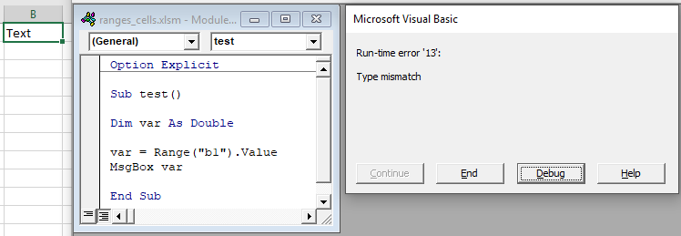
Other Cell Value Examples
VBA Programming | Code Generator does work for you!
Copy Cell Value
It’s easy to set a cell value equal to another cell value (or “Copy” a cell value):
Range("A1").Value = Range("B1").ValueYou can even do this with ranges of cells (the ranges must be the same size):
Range("A1:A5").Value = Range("B1:B5").ValueCompare Cell Values
You can compare cell values using the standard comparison operators.
Test if cell values are equal:
MsgBox Range("A1").Value = Range("B1").ValueWill return TRUE if cell values are equal. Otherwise FALSE.
You can also create an If Statement to compare cell values:
If Range("A1").Value > Range("B1").Value Then

  Range("C1").Value = "Greater Than"

Elseif Range("A1").Value = Range("B1").Value Then

  Range("C1").Value = "Equal"

Else

  Range("C1").Value = "Less Than"

End If
You can compare text in the same way (Remember that VBA is Case Sensitive)
В приложении Excel все данные как правило находятся в ячейках на листах, с которыми макросы работают как с базой данных. Поэтому, начинающему программисту VBA важно понимать как читать значения из ячейки Excel в переменные или массивы и, наоборот, записывать какие-либо значения на лист в ячейки.
Обращение к конкретной ячейке
Прежде чем читать или записывать значение в ячейке, нужно определиться с тем, как можно указать какая именно ячейка нам необходима.
Полный путь к ячейке A1 в Книге1 на Листе1 можно записать двумя вариантами:
- С помощью Range
- С помощью Cells
Пример 1: Обратиться к ячейке A3 находящейся в Книге1 на Листе1
Workbooks("Книга1.xls").Sheets("Лист1").Range("A3") ' Обратиться к ячейке A3
Workbooks("Книга1.xls").Sheets("Лист1").Cells(3, 1) ' Обратиться к ячейке в 3-й строке и 1-й колонке (A3)
Однако, как правило, полный путь редко используется, т.к. макрос работает с Книгой, в которой он записан и часто на активном листе. Поэтому путь к ячейке можно сократить и написать просто:
Пример 2: Обратиться к ячейке A1 в текущей книге на активном листе
Range("A1")
Cells(1, 1)
Если всё же путь к книге или листу необходим, но не хочется его писать при каждом обращении к ячейкам, можно использовать конструкцию With End With. При этом, обращаясь к ячейкам, необходимо использовать в начале «.» (точку).
Пример 3: Обратиться к ячейке A1 и B1 в Книге1 на Листе2.
With Workbooks("Книга1").Sheets("Лист2")
  ' Вывести значение ячейки A1, которая находится на Листе2
  MsgBox .Range("A1")
  ' Вывести значение ячейки B1, которая находится на Листе2
  MsgBox .Range("B1")
End With
Так же, можно обратиться и к активной (выбранной в данный момент времени) ячейке.
Пример 4: Обратиться к активной ячейке на Листе3 текущей книги.
Application.ActiveCell ' полная запись
ActiveCell ' краткая запись
Чтение значения из ячейки
Есть 3 способа получения значения ячейки, каждый из которых имеет свои особенности:
- Value2 — базовое значение ячейки, т.е. как оно хранится в самом Excel-е. В связи с чем, например, дата будет прочтена как число от 1 до 2958466, а время будет прочитано как дробное число. Value2 — самый быстрый способ чтения значения, т.к. не происходит никаких преобразований.
- Value — значение ячейки, приведенное к типу ячейки. Если ячейка хранит дату, будет приведено к типу Date. Если ячейка отформатирована как валюта, будет преобразована к типу Currency (в связи с чем, знаки с 5-го и далее будут усечены).
- Text — визуальное отображение значения ячейки. Например, если ячейка, содержит дату в виде «число месяц прописью год», то Text (в отличие от Value и Value2) именно в таком виде и вернет значение. Использовать Text нужно осторожно, т.к., если, например, значение не входит в ячейку и отображается в виде «#####» то Text вернет вам не само значение, а эти самые «решетки».
По-умолчанию, если при обращении к ячейке не указывать способ чтения значения, то используется способ Value.
Пример 5: В ячейке A1 активного листа находится дата 01.03.2018. Для ячейки выбран формат «14 марта 2001 г.». Необходимо прочитать значение ячейки всеми перечисленными выше способами и отобразить в диалоговом окне.
MsgBox Cells(1, 1)        ' выведет 01.03.2018
MsgBox Cells(1, 1).Value  ' выведет 01.03.2018
MsgBox Cells(1, 1).Value2 ' выведет 43160
MsgBox Cells(1, 1).Text   ' выведет 01 марта 2018 г.

Dim d As Date
d = Cells(1, 1).Value2    ' числовое представление даты преобразуется в тип Date
MsgBox d                  ' выведет 01.03.2018
Пример 6: В ячейке С1 активного листа находится значение 123,456789. Для ячейки выбран формат «Денежный» с 3 десятичными знаками. Необходимо прочитать значение ячейки всеми перечисленными выше способами и отобразить в диалоговом окне.
MsgBox Range("C1")        ' выведет 123,4568
MsgBox Range("C1").Value  ' выведет 123,4568
MsgBox Range("C1").Value2 ' выведет 123,456789
MsgBox Range("C1").Text   ' выведет 123,457р.

Dim c As Currency
c = Range("C1").Value2    ' значение преобразуется в тип Currency
MsgBox c                  ' выведет 123,4568

Dim d As Double
d = Range("C1").Value2    ' значение преобразуется в тип Double
MsgBox d                  ' выведет 123,456789
При присвоении значения переменной или элементу массива, необходимо учитывать тип переменной. Например, если оператором Dim задан тип Integer, а в ячейке находится текст, при выполнении произойдет ошибка «Type mismatch». Как определить тип значения в ячейке, рассказано в следующей статье.
Пример 7: В ячейке B1 активного листа находится текст. Прочитать значение ячейки в переменную.
Dim s As String
Dim i As Integer
s = Range("B1").Value2 ' успех
i = Range("B1").Value2 ' ошибка
Таким образом, разница между Text, Value и Value2 в способе получения значения. Очевидно, что Value2 наиболее предпочтителен, но при преобразовании даты в текст (например, чтобы показать значение пользователю), нужно использовать функцию Format.
Запись значения в ячейку
Осуществить запись значения в ячейку можно 2 способами: с помощью Value и Value2. Использование Text для записи значения не возможно, т.к. это свойство только для чтения.
Пример 8: Записать в ячейку A1 активного листа значение 123,45
Range("A1") = 123.45
Range("A1").Value = 123.45
Range("A1").Value2 = 123.45
Все три строки запишут в A1 одно и то же значение.
Пример 9: Записать в ячейку A2 активного листа дату 1 марта 2018 года
Cells(2, 1) = #3/1/2018#
Cells(2, 1).Value = #3/1/2018#
Cells(2, 1).Value2 = #3/1/2018#
В данном примере тоже запишется одно и то же значение в ячейку A2 активного листа.
Визуальное отображение значения на экране будет зависеть от того, какой формат ячейки выбран на листе.
Обращение к ячейке на листе Excel из кода VBA по адресу, индексу и имени. Чтение информации из ячейки. Очистка значения ячейки. Метод ClearContents объекта Range.
Обращение к ячейке по адресу
Допустим, у нас есть два открытых файла: «Книга1» и «Книга2», причем, файл «Книга1» активен и в нем находится исполняемый код VBA.
В общем случае при обращении к ячейке неактивной рабочей книги «Книга2» из кода файла «Книга1» прописывается полный путь:
|
Workbooks(«Книга2.xlsm»).Sheets(«Лист2»).Range(«C5») Workbooks(«Книга2.xlsm»).Sheets(«Лист2»).Cells(5, 3) Workbooks(«Книга2.xlsm»).Sheets(«Лист2»).Cells(5, «C») Workbooks(«Книга2.xlsm»).Sheets(«Лист2»).[C5] |
Удобнее обращаться к ячейке через свойство рабочего листа Cells(номер строки, номер столбца), так как вместо номеров строк и столбцов можно использовать переменные. Обратите внимание, что при обращении к любой рабочей книге, она должна быть открыта, иначе произойдет ошибка. Закрытую книгу перед обращением к ней необходимо открыть.
Теперь предположим, что у нас в активной книге «Книга1» активны «Лист1» и ячейка на нем «A1». Тогда обращение к ячейке «A1» можно записать следующим образом:
|
ActiveCell Range(«A1») Cells(1, 1) Cells(1, «A») [A1] |
Точно также можно обращаться и к другим ячейкам активного рабочего листа, кроме обращения ActiveCell, так как активной может быть только одна ячейка, в нашем примере – это ячейка «A1».
Если мы обращаемся к ячейке на неактивном листе активной рабочей книги, тогда необходимо указать этот лист:
|
‘по основному имени листа Лист2.Cells(2, 7) ‘по имени ярлыка Sheets(«Имя ярлыка»).Cells(3, 8) |
Имя ярлыка может совпадать с основным именем листа. Увидеть эти имена можно в окне редактора VBA в проводнике проекта. Без скобок отображается основное имя листа, в скобках – имя ярлыка.
Обращение к ячейке по индексу
К ячейке на рабочем листе можно обращаться по ее индексу (порядковому номеру), который считается по расположению ячейки на листе слева-направо и сверху-вниз.
Например, индекс ячеек в первой строке равен номеру столбца. Индекс ячеек во второй строке равен количеству ячеек в первой строке (которое равно общему количеству столбцов на листе, зависящему от версии Excel) плюс номер столбца. Индекс ячеек в третьей строке равен количеству ячеек в двух первых строках плюс номер столбца. И так далее.
Для примера, Cells(4) та же ячейка, что и Cells(1, 4). Используется такое обозначение редко, тем более, что у разных версий Excel может быть разным количество столбцов и строк на рабочем листе.
По индексу можно обращаться к ячейке не только на всем рабочем листе, но и в отдельном диапазоне. Нумерация ячеек осуществляется в пределах заданного диапазона по тому же правилу: слева-направо и сверху-вниз. Вот индексы ячеек диапазона Range(«A1:C3»):

Обращение к ячейке Range("A1:C3").Cells(5) соответствует выражению Range("B2").
Обращение к ячейке по имени
Если ячейке на рабочем листе Excel присвоено имя (Формулы –> Присвоить имя), то обращаться к ней можно по присвоенному имени.
Допустим одной из ячеек присвоено имя – «Итого», тогда обратиться к ней можно – Range("Итого").
Запись информации в ячейку
Содержание ячейки определяется ее свойством «Value», которое в VBA Excel является свойством по умолчанию и его можно явно не указывать. Записывается информация в ячейку при помощи оператора присваивания «=»:
|
Cells(2, 4).Value = 15 Cells(2, 4) = 15 Range(«A1») = «Этот текст записываем в ячейку» ActiveCell = 28 + 10*36 |
Вместе с числами и текстом можно использовать переменные. Примеры здесь и ниже приведены для активного листа. Для неактивных листов дополнительно необходимо указывать имя листа, как в разделе «Обращение к ячейке».
Чтение информации из ячейки
Считать информацию из ячейки в переменную можно также при помощи оператора присваивания «=»:
|
Sub Test() Dim a1 As Integer, a2 As Integer, a3 As Integer Range(«A3») = 6 Cells(2, 5) = 15 a1 = Range(«A3») a2 = Cells(2, 5) a3 = a1 * a2 MsgBox a3 End Sub |
Точно также можно обмениваться информацией между ячейками:
|
Cells(2, 2) = Range(«A4») |
Очистка значения ячейки
Очищается ячейка от значения с помощью метода ClearContents. Кроме того, можно присвоить ячейке значение нуля. пустой строки или Empty:
|
Cells(10, 2).ClearContents Range(«D23») = 0 ActiveCell = «» Cells(5, «D») = Empty |
A cell is an individual cell and is also a part of a range. Technically, there are two methods to interact with a cell in VBA: the range method and the cell method. We can use the range method like range(“A2”). The value will give us the value of the A2 cell, or we can use the cell method as cells(2,1). The value will also give us the value of A2 cells.
Be it Excel or VBA, we all need to work with cells because it will store all the data in cells. So, it all boils down to how well we know about cells in VBA. So, if cells are such a crucial part of the VBA, then it is important to understand them well. So, if you are a starter regarding VBA cells, this article will guide you on how to get cell values in Excel VBA in detail.
First, we can reference or work with cells in VBA in two ways: using CELLS propertyCells are cells of the worksheet, and in VBA, when we refer to cells as a range property, we refer to the same cells. In VBA concepts, cells are also the same, no different from normal excel cells.read more and RANGE object. Of course, why CELLS is a property and why RANGE is an object is a different analogy. Later in the article, we will get to that point.
Table of contents
- Get Cell Value with Excel VBA
- Examples of getting Cell Value in Excel VBA
- Example #1 – Using RANGE or CELLS Property
- Example #2 – Get Value from Cell in Excel VBA
- Example #3 – Get Value from One Cell to Another Cell
- Things to Remember
- Recommended Articles
- Examples of getting Cell Value in Excel VBA
You are free to use this image on your website, templates, etc, Please provide us with an attribution linkArticle Link to be Hyperlinked
For eg:
Source: Get Cell Value in Excel VBA (wallstreetmojo.com)
Examples of getting Cell Value in Excel VBA
Below are the examples of getting cell values in Excel VBA.
You can download this VBA Get Cell Value Excel Template here – VBA Get Cell Value Excel Template
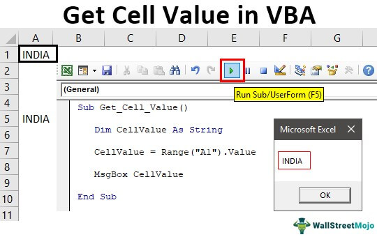
Example #1 – Using RANGE or CELLS Property
In cell A1 we have a value of “India.”

We can reference this cell with a CELLS property or RANGE object. Let us see both of them in detail.
Using Range Property
First, start the macro procedure.
Code:
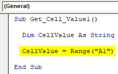
Sub Get_Cell_Value()

End Sub

Now open the RANGE object.
Code:
Sub Get_Cell_Value()

Range(

End Sub

The first argument of this object is “Cell1,” which is the cell we are referring to. In this case, it is cell A1, so we need to supply the cell address in double quotes for the RANGE object.
Code:
Sub Get_Cell_Value()

Range("A1")

End Sub

Since only one cell refers to other parameters is irrelevant, close the bracket and put a dot to see the IntelliSense list.

As you can see above, the moment we put a dot, we can see all the available IntelliSense lists of properties and methods of range objects.
Since we are selecting the cell, we need to choose the “SELECT” method from the IntelliSense list.
Code:
Sub Get_Cell_Value()

Range("A1").Select

End Sub

Now, select the cell other than A1 and run the code.
It does not matter which cell you select when you run the code. It has chosen the mentioned cell, i.e., the A1 cell.
Using Cells Property
Similarly, we use the CELLS property now.
Code:
Sub Get_Cell_Value()

Range("A1").Select
Cells(

End Sub

Unlike the RANGE object, we could directly supply the cell address. However, using this CELLS property, we cannot do that.
The first argument of this property is “Row Index,” i.e., which row we are referring to. Since we are selecting cell A1 we are referring to the first row, so mention 1.

The next argument is the “Column Index,” i.e., which column we refer to. For example, the A1 cell column is the first column, so enter 1.

Our code reads CELLS (1, 1) i.e. first row first column = A1.
Now, put a dot and see whether you get to see the IntelliSense list or not.

We cannot see any IntelliSense list with CELLS properties, so we must be sure what we are writing. Enter “Select” as the method.
Code:
Sub Get_Cell_Value()

Range("A1").Select
Cells(1, 1).Select

End Sub

This will also select cell A1.
Example #2 – Get Value from Cell in Excel VBA
Selecting is the first thing we have learned. Now, we will see how to get value from cells. Before we select the cell, we need to define the variable to store the value from the cell.
Code:
Sub Get_Cell_Value1()

Dim CellValue As String

End Sub

Now, mention the cell address using either the RANGE object or the CELLS property. Since you are a beginner, use the RANGE object only because we can see the IntelliSense list with the RANGE object.
For the defined variable, put an equal sign and mention the cell address.
Code:
Sub Get_Cell_Value1()

Dim CellValue As String

CellValue = Range("A1")

End Sub
Once again, put a dot to see the IntelliSense list.
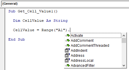
From the VBA IntelliSense list, choose the “Value” property to get the value from the mentioned cell.
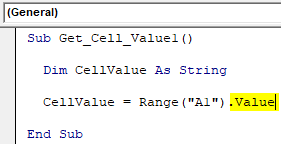
Code:
Sub Get_Cell_Value1()

Dim CellValue As String

CellValue = Range("A1").Value

End Sub
Now, the variable “CellValue” holds the value from cell A1. Show this variable value in the message box in VBA.
Code:
Sub Get_Cell_Value1()

Dim CellValue As String

CellValue = Range("A1").Value

MsgBox CellValue

End Sub

Run the code and see the result in a message box.
Since there is a value of “INDIA” in cell A1, the same thing also appeared in the message box. Like this, we can get the value of the cell by the VBA valueIn VBA, the value property is usually used alongside the range method to assign a value to a range. It’s a VBA built-in expression that we can use with other functions.read more of the cell.
Example #3 – Get Value from One Cell to Another Cell
We know how to get value from the cell using VBA. Now, the question is how to insert a value into the cell. Let us take the same example only. For cell A1, we need to insert the value of “INDIA,” which we can do from the code below.
Code:
Sub Get_Cell_Value2()

Range("A1").Value = "INDIA"

End Sub

It will insert the value of “INDIA” to cell A1. Similarly, we can write the code below to get value from one cell to another.
Code:
Sub Get_Cell_Value2()

Range("A5").Value = Range("A1").Value

End Sub

Let me explain the code to you.
For cell A5, we need the value from the cell A1 value; that’s all this code says. So, this will get the value from cell A1 to A5 using VBA codeVBA code refers to a set of instructions written by the user in the Visual Basic Applications programming language on a Visual Basic Editor (VBE) to perform a specific task.read more.

Things to Remember
- Inserting value to cells and getting value from the cell requires the VBA “VALUE” property to be used.
- We can select only one cell using the CELLS property but use the RANGE object. Likewise, we can select multiple cells.
Recommended Articles
This article has been a guide to Get Cell Value in Excel VBA. Here, we discuss the examples of getting cell values using a range of cell properties in Excel VBA and a downloadable Excel template. Below you can find some useful Excel VBA articles: –
- VBA Variable Range
- Split String into Array in VBA
- Range Cells in VBA
- Active Cell in VBA
“It is a capital mistake to theorize before one has data”- Sir Arthur Conan Doyle
This post covers everything you need to know about using Cells and Ranges in VBA. You can read it from start to finish as it is laid out in a logical order. If you prefer you can use the table of contents below to go to a section of your choice.
Topics covered include Offset property, reading values between cells, reading values to arrays and formatting cells.
A Quick Guide to Ranges and Cells
| Function | Takes | Returns | Example | Gives |
|---|---|---|---|---|
|
Range |
cell address | multiple cells | .Range(«A1:A4») | $A$1:$A$4 |
| Cells | row, column | one cell | .Cells(1,5) | $E$1 |
| Offset | row, column | multiple cells | Range(«A1:A2») .Offset(1,2) |
$C$2:$C$3 |
| Rows | row(s) | one or more rows | .Rows(4) .Rows(«2:4») |
$4:$4 $2:$4 |
| Columns | column(s) | one or more columns | .Columns(4) .Columns(«B:D») |
$D:$D $B:$D |
Download the Code
The Webinar
If you are a member of the VBA Vault, then click on the image below to access the webinar and the associated source code.
(Note: Website members have access to the full webinar archive.)

Introduction
This is the third post dealing with the three main elements of VBA. These three elements are the Workbooks, Worksheets and Ranges/Cells. Cells are by far the most important part of Excel. Almost everything you do in Excel starts and ends with Cells.
Generally speaking, you do three main things with Cells
- Read from a cell.
- Write to a cell.
- Change the format of a cell.
Excel has a number of methods for accessing cells such as Range, Cells and Offset.These can cause confusion as they do similar things and can lead to confusion
In this post I will tackle each one, explain why you need it and when you should use it.
Let’s start with the simplest method of accessing cells – using the Range property of the worksheet.
Important Notes
I have recently updated this article so that is uses Value2.
You may be wondering what is the difference between Value, Value2 and the default:
' Value2
Range("A1").Value2 = 56

' Value
Range("A1").Value = 56

' Default uses value
Range("A1") = 56
Using Value may truncate number if the cell is formatted as currency. If you don’t use any property then the default is Value.
It is better to use Value2 as it will always return the actual cell value(see this article from Charle Williams.)
The Range Property
The worksheet has a Range property which you can use to access cells in VBA. The Range property takes the same argument that most Excel Worksheet functions take e.g. “A1”, “A3:C6” etc.
The following example shows you how to place a value in a cell using the Range property.
' https://excelmacromastery.com/
Public Sub WriteToCell()

    ' Write number to cell A1 in sheet1 of this workbook
    ThisWorkbook.Worksheets("Sheet1").Range("A1").Value2 = 67

    ' Write text to cell A2 in sheet1 of this workbook
    ThisWorkbook.Worksheets("Sheet1").Range("A2").Value2 = "John Smith"

    ' Write date to cell A3 in sheet1 of this workbook
    ThisWorkbook.Worksheets("Sheet1").Range("A3").Value2 = #11/21/2017#

End Sub
As you can see Range is a member of the worksheet which in turn is a member of the Workbook. This follows the same hierarchy as in Excel so should be easy to understand. To do something with Range you must first specify the workbook and worksheet it belongs to.
For the rest of this post I will use the code name to reference the worksheet.

The following code shows the above example using the code name of the worksheet i.e. Sheet1 instead of ThisWorkbook.Worksheets(“Sheet1”).
' https://excelmacromastery.com/
Public Sub UsingCodeName()

    ' Write number to cell A1 in sheet1 of this workbook
    Sheet1.Range("A1").Value2 = 67

    ' Write text to cell A2 in sheet1 of this workbook
    Sheet1.Range("A2").Value2 = "John Smith"

    ' Write date to cell A3 in sheet1 of this workbook
    Sheet1.Range("A3").Value2 = #11/21/2017#

End Sub
You can also write to multiple cells using the Range property
' https://excelmacromastery.com/
Public Sub WriteToMulti()

    ' Write number to a range of cells
    Sheet1.Range("A1:A10").Value2 = 67

    ' Write text to multiple ranges of cells
    Sheet1.Range("B2:B5,B7:B9").Value2 = "John Smith"

End Sub
You can download working examples of all the code from this post from the top of this article.
The Cells Property of the Worksheet
The worksheet object has another property called Cells which is very similar to range. There are two differences
- Cells returns a range of one cell only.
- Cells takes row and column as arguments.
The example below shows you how to write values to cells using both the Range and Cells property
' https://excelmacromastery.com/
Public Sub UsingCells()

    ' Write to A1
    Sheet1.Range("A1").Value2 = 10
    Sheet1.Cells(1, 1).Value2  = 10

    ' Write to A10
    Sheet1.Range("A10").Value2 = 10
    Sheet1.Cells(10, 1).Value2  = 10

    ' Write to E1
    Sheet1.Range("E1").Value2 = 10
    Sheet1.Cells(1, 5).Value2  = 10

End Sub
You may be wondering when you should use Cells and when you should use Range. Using Range is useful for accessing the same cells each time the Macro runs.
For example, if you were using a Macro to calculate a total and write it to cell A10 every time then Range would be suitable for this task.
Using the Cells property is useful if you are accessing a cell based on a number that may vary. It is easier to explain this with an example.
In the following code, we ask the user to specify the column number. Using Cells gives us the flexibility to use a variable number for the column.
' https://excelmacromastery.com/
Public Sub WriteToColumn()

    Dim UserCol As Integer

    ' Get the column number from the user
    UserCol = Application.InputBox(" Please enter the column...", Type:=1)

    ' Write text to user selected column
    Sheet1.Cells(1, UserCol).Value2 = "John Smith"

End Sub
In the above example, we are using a number for the column rather than a letter.
To use Range here would require us to convert these values to the letter/number cell reference e.g. “C1”. Using the Cells property allows us to provide a row and a column number to access a cell.
Sometimes you may want to return more than one cell using row and column numbers. The next section shows you how to do this.
Using Cells and Range together
As you have seen you can only access one cell using the Cells property. If you want to return a range of cells then you can use Cells with Ranges as follows
' https://excelmacromastery.com/
Public Sub UsingCellsWithRange()

    With Sheet1
        ' Write 5 to Range A1:A10 using Cells property
        .Range(.Cells(1, 1), .Cells(10, 1)).Value2 = 5

        ' Format Range B1:Z1 to be bold
        .Range(.Cells(1, 2), .Cells(1, 26)).Font.Bold = True

    End With

End Sub
As you can see, you provide the start and end cell of the Range. Sometimes it can be tricky to see which range you are dealing with when the value are all numbers. Range has a property called Address which displays the letter/ number cell reference of any range. This can come in very handy when you are debugging or writing code for the first time.
In the following example we print out the address of the ranges we are using:
' https://excelmacromastery.com/
Public Sub ShowRangeAddress()

    ' Note: Using underscore allows you to split up lines of code
    With Sheet1

        ' Write 5 to Range A1:A10 using Cells property
        .Range(.Cells(1, 1), .Cells(10, 1)).Value2 = 5
        Debug.Print "First address is : " _
            + .Range(.Cells(1, 1), .Cells(10, 1)).Address

        ' Format Range B1:Z1 to be bold
        .Range(.Cells(1, 2), .Cells(1, 26)).Font.Bold = True
        Debug.Print "Second address is : " _
            + .Range(.Cells(1, 2), .Cells(1, 26)).Address

    End With

End Sub
In the example I used Debug.Print to print to the Immediate Window. To view this window select View->Immediate Window(or Ctrl G)


You can download all the code for this post from the top of this article.
The Offset Property of Range
Range has a property called Offset. The term Offset refers to a count from the original position. It is used a lot in certain areas of programming. With the Offset property you can get a Range of cells the same size and a certain distance from the current range. The reason this is useful is that sometimes you may want to select a Range based on a certain condition. For example in the screenshot below there is a column for each day of the week. Given the day number(i.e. Monday=1, Tuesday=2 etc.) we need to write the value to the correct column.

We will first attempt to do this without using Offset.
' https://excelmacromastery.com/
' This sub tests with different values
Public Sub TestSelect()

    ' Monday
    SetValueSelect 1, 111.21
    ' Wednesday
    SetValueSelect 3, 456.99
    ' Friday
    SetValueSelect 5, 432.25
    ' Sunday
    SetValueSelect 7, 710.17

End Sub

' Writes the value to a column based on the day
Public Sub SetValueSelect(lDay As Long, lValue As Currency)

    Select Case lDay
        Case 1: Sheet1.Range("H3").Value2 = lValue
        Case 2: Sheet1.Range("I3").Value2 = lValue
        Case 3: Sheet1.Range("J3").Value2 = lValue
        Case 4: Sheet1.Range("K3").Value2 = lValue
        Case 5: Sheet1.Range("L3").Value2 = lValue
        Case 6: Sheet1.Range("M3").Value2 = lValue
        Case 7: Sheet1.Range("N3").Value2 = lValue
    End Select

End Sub
As you can see in the example, we need to add a line for each possible option. This is not an ideal situation. Using the Offset Property provides a much cleaner solution
' https://excelmacromastery.com/
' This sub tests with different values
Public Sub TestOffset()

    DayOffSet 1, 111.01
    DayOffSet 3, 456.99
    DayOffSet 5, 432.25
    DayOffSet 7, 710.17

End Sub

Public Sub DayOffSet(lDay As Long, lValue As Currency)

    ' We use the day value with offset specify the correct column
    Sheet1.Range("G3").Offset(, lDay).Value2 = lValue

End Sub
As you can see this solution is much better. If the number of days in increased then we do not need to add any more code. For Offset to be useful there needs to be some kind of relationship between the positions of the cells. If the Day columns in the above example were random then we could not use Offset. We would have to use the first solution.
One thing to keep in mind is that Offset retains the size of the range. So .Range(“A1:A3”).Offset(1,1) returns the range B2:B4. Below are some more examples of using Offset
' https://excelmacromastery.com/
Public Sub UsingOffset()

    ' Write to B2 - no offset
    Sheet1.Range("B2").Offset().Value2 = "Cell B2"

    ' Write to C2 - 1 column to the right
    Sheet1.Range("B2").Offset(, 1).Value2 = "Cell C2"

    ' Write to B3 - 1 row down
    Sheet1.Range("B2").Offset(1).Value2 = "Cell B3"

    ' Write to C3 - 1 column right and 1 row down
    Sheet1.Range("B2").Offset(1, 1).Value2 = "Cell C3"

    ' Write to A1 - 1 column left and 1 row up
    Sheet1.Range("B2").Offset(-1, -1).Value2 = "Cell A1"

    ' Write to range E3:G13 - 1 column right and 1 row down
    Sheet1.Range("D2:F12").Offset(1, 1).Value2 = "Cells E3:G13"

End Sub
Using the Range CurrentRegion
CurrentRegion returns a range of all the adjacent cells to the given range.
In the screenshot below you can see the two current regions. I have added borders to make the current regions clear.

A row or column of blank cells signifies the end of a current region.
You can manually check the CurrentRegion in Excel by selecting a range and pressing Ctrl + Shift + *.
If we take any range of cells within the border and apply CurrentRegion, we will get back the range of cells in the entire area.
For example
Range(“B3”).CurrentRegion will return the range B3:D14
Range(“D14”).CurrentRegion will return the range B3:D14
Range(“C8:C9”).CurrentRegion will return the range B3:D14
and so on
How to Use
We get the CurrentRegion as follows
' Current region will return B3:D14 from above example
Dim rg As Range
Set rg = Sheet1.Range("B3").CurrentRegion
Read Data Rows Only
Read through the range from the second row i.e.skipping the header row
' Current region will return B3:D14 from above example
Dim rg As Range
Set rg = Sheet1.Range("B3").CurrentRegion

' Start at row 2 - row after header
Dim i As Long
For i = 2 To rg.Rows.Count
    ' current row, column 1 of range
    Debug.Print rg.Cells(i, 1).Value2
Next i
Remove Header
Remove header row(i.e. first row) from the range. For example if range is A1:D4 this will return A2:D4
' Current region will return B3:D14 from above example
Dim rg As Range
Set rg = Sheet1.Range("B3").CurrentRegion

' Remove Header
Set rg = rg.Resize(rg.Rows.Count - 1).Offset(1)

' Start at row 1 as no header row
Dim i As Long
For i = 1 To rg.Rows.Count
    ' current row, column 1 of range
    Debug.Print rg.Cells(i, 1).Value2
Next i
Using Rows and Columns as Ranges
If you want to do something with an entire Row or Column you can use the Rows or Columns property of the Worksheet. They both take one parameter which is the row or column number you wish to access
' https://excelmacromastery.com/
Public Sub UseRowAndColumns()

    ' Set the font size of column B to 9
    Sheet1.Columns(2).Font.Size = 9

    ' Set the width of columns D to F
    Sheet1.Columns("D:F").ColumnWidth = 4

    ' Set the font size of row 5 to 18
    Sheet1.Rows(5).Font.Size = 18

End Sub
Using Range in place of Worksheet
You can also use Cells, Rows and Columns as part of a Range rather than part of a Worksheet. You may have a specific need to do this but otherwise I would avoid the practice. It makes the code more complex. Simple code is your friend. It reduces the possibility of errors.
The code below will set the second column of the range to bold. As the range has only two rows the entire column is considered B1:B2
' https://excelmacromastery.com/
Public Sub UseColumnsInRange()

    ' This will set B1 and B2 to be bold
    Sheet1.Range("A1:C2").Columns(2).Font.Bold = True

End Sub
You can download all the code for this post from the top of this article.
Reading Values from one Cell to another
In most of the examples so far we have written values to a cell. We do this by placing the range on the left of the equals sign and the value to place in the cell on the right. To write data from one cell to another we do the same. The destination range goes on the left and the source range goes on the right.
The following example shows you how to do this:
' https://excelmacromastery.com/
Public Sub ReadValues()

    ' Place value from B1 in A1
    Sheet1.Range("A1").Value2 = Sheet1.Range("B1").Value2

    ' Place value from B3 in sheet2 to cell A1
    Sheet1.Range("A1").Value2 = Sheet2.Range("B3").Value2

    ' Place value from B1 in cells A1 to A5
    Sheet1.Range("A1:A5").Value2 = Sheet1.Range("B1").Value2

    ' You need to use the "Value" property to read multiple cells
    Sheet1.Range("A1:A5").Value2 = Sheet1.Range("B1:B5").Value2

End Sub
As you can see from this example it is not possible to read from multiple cells. If you want to do this you can use the Copy function of Range with the Destination parameter
' https://excelmacromastery.com/
Public Sub CopyValues()

    ' Store the copy range in a variable
    Dim rgCopy As Range
    Set rgCopy = Sheet1.Range("B1:B5")

    ' Use this to copy from more than one cell
    rgCopy.Copy Destination:=Sheet1.Range("A1:A5")

    ' You can paste to multiple destinations
    rgCopy.Copy Destination:=Sheet1.Range("A1:A5,C2:C6")

End Sub
The Copy function copies everything including the format of the cells. It is the same result as manually copying and pasting a selection. You can see more about it in the Copying and Pasting Cells section.
Using the Range.Resize Method
When copying from one range to another using assignment(i.e. the equals sign), the destination range must be the same size as the source range.
Using the Resize function allows us to resize a range to a given number of rows and columns.
For example:
' https://excelmacromastery.com/
Sub ResizeExamples()

    ' Prints A1
    Debug.Print Sheet1.Range("A1").Address

    ' Prints A1:A2
    Debug.Print Sheet1.Range("A1").Resize(2, 1).Address

    ' Prints A1:A5
    Debug.Print Sheet1.Range("A1").Resize(5, 1).Address

    ' Prints A1:D1
    Debug.Print Sheet1.Range("A1").Resize(1, 4).Address

    ' Prints A1:C3
    Debug.Print Sheet1.Range("A1").Resize(3, 3).Address

End Sub
When we want to resize our destination range we can simply use the source range size.
In other words, we use the row and column count of the source range as the parameters for resizing:
' https://excelmacromastery.com/
Sub Resize()

    Dim rgSrc As Range, rgDest As Range

    ' Get all the data in the current region
    Set rgSrc = Sheet1.Range("A1").CurrentRegion

      ' Get the range destination
    Set rgDest = Sheet2.Range("A1")
    Set rgDest = rgDest.Resize(rgSrc.Rows.Count, rgSrc.Columns.Count)

    rgDest.Value2 = rgSrc.Value2

End Sub
We can do the resize in one line if we prefer:
' https://excelmacromastery.com/
Sub ResizeOneLine()

    Dim rgSrc As Range

    ' Get all the data in the current region
    Set rgSrc = Sheet1.Range("A1").CurrentRegion

    With rgSrc
        Sheet2.Range("A1").Resize(.Rows.Count, .Columns.Count).Value2 = .Value2
    End With

End Sub
Reading Values to variables
We looked at how to read from one cell to another. You can also read from a cell to a variable. A variable is used to store values while a Macro is running. You normally do this when you want to manipulate the data before writing it somewhere. The following is a simple example using a variable. As you can see the value of the item to the right of the equals is written to the item to the left of the equals.
' https://excelmacromastery.com/
Public Sub UseVariables()

    ' Create
    Dim number As Long

    ' Read number from cell
    number = Sheet1.Range("A1").Value2

    ' Add 1 to value
    number = number + 1

    ' Write new value to cell
    Sheet1.Range("A2").Value2 = number

End Sub
To read text to a variable you use a variable of type String:
' https://excelmacromastery.com/
Public Sub UseVariableText()

    ' Declare a variable of type string
    Dim text As String

    ' Read value from cell
    text = Sheet1.Range("A1").Value2

    ' Write value to cell
    Sheet1.Range("A2").Value2 = text

End Sub
You can write a variable to a range of cells. You just specify the range on the left and the value will be written to all cells in the range.
' https://excelmacromastery.com/
Public Sub VarToMulti()

    ' Read value from cell
    Sheet1.Range("A1:B10").Value2 = 66

End Sub
You cannot read from multiple cells to a variable. However you can read to an array which is a collection of variables. We will look at doing this in the next section.
How to Copy and Paste Cells
If you want to copy and paste a range of cells then you do not need to select them. This is a common error made by new VBA users.
Note: We normally use Range.Copy when we want to copy formats, formulas, validation. If we want to copy values it is not the most efficient method.
I have written a complete guide to copying data in Excel VBA here.
You can simply copy a range of cells like this:
Range("A1:B4").Copy Destination:=Range("C5")
Using this method copies everything – values, formats, formulas and so on. If you want to copy individual items you can use the PasteSpecial property of range.
It works like this
Range("A1:B4").Copy
Range("F3").PasteSpecial Paste:=xlPasteValues
Range("F3").PasteSpecial Paste:=xlPasteFormats
Range("F3").PasteSpecial Paste:=xlPasteFormulas
The following table shows a full list of all the paste types
| Paste Type |
|---|
| xlPasteAll |
| xlPasteAllExceptBorders |
| xlPasteAllMergingConditionalFormats |
| xlPasteAllUsingSourceTheme |
| xlPasteColumnWidths |
| xlPasteComments |
| xlPasteFormats |
| xlPasteFormulas |
| xlPasteFormulasAndNumberFormats |
| xlPasteValidation |
| xlPasteValues |
| xlPasteValuesAndNumberFormats |
Reading a Range of Cells to an Array
You can also copy values by assigning the value of one range to another.
Range("A3:Z3").Value2 = Range("A1:Z1").Value2
The value of range in this example is considered to be a variant array. What this means is that you can easily read from a range of cells to an array. You can also write from an array to a range of cells. If you are not familiar with arrays you can check them out in this post.
The following code shows an example of using an array with a range:
' https://excelmacromastery.com/
Public Sub ReadToArray()

    ' Create dynamic array
    Dim StudentMarks() As Variant

    ' Read 26 values into array from the first row
    StudentMarks = Range("A1:Z1").Value2

    ' Do something with array here

    ' Write the 26 values to the third row
    Range("A3:Z3").Value2 = StudentMarks

End Sub
Keep in mind that the array created by the read is a 2 dimensional array. This is because a spreadsheet stores values in two dimensions i.e. rows and columns
Going through all the cells in a Range
Sometimes you may want to go through each cell one at a time to check value.
You can do this using a For Each loop shown in the following code
' https://excelmacromastery.com/
Public Sub TraversingCells()

    ' Go through each cells in the range
    Dim rg As Range
    For Each rg In Sheet1.Range("A1:A10,A20")
        ' Print address of cells that are negative
        If rg.Value < 0 Then
            Debug.Print rg.Address + " is negative."
        End If
    Next

End Sub
You can also go through consecutive Cells using the Cells property and a standard For loop.
The standard loop is more flexible about the order you use but it is slower than a For Each loop.
' https://excelmacromastery.com/
Public Sub TraverseCells()

    ' Go through cells from A1 to A10
    Dim i As Long
    For i = 1 To 10
        ' Print address of cells that are negative
        If Range("A" & i).Value < 0 Then
            Debug.Print Range("A" & i).Address + " is negative."
        End If
    Next

    ' Go through cells in reverse i.e. from A10 to A1
    For i = 10 To 1 Step -1
        ' Print address of cells that are negative
        If Range("A" & i) < 0 Then
            Debug.Print Range("A" & i).Address + " is negative."
        End If
    Next

End Sub
Formatting Cells
Sometimes you will need to format the cells the in spreadsheet. This is actually very straightforward. The following example shows you various formatting you can add to any range of cells
' https://excelmacromastery.com/
Public Sub FormattingCells()

    With Sheet1

        ' Format the font
        .Range("A1").Font.Bold = True
        .Range("A1").Font.Underline = True
        .Range("A1").Font.Color = rgbNavy

        ' Set the number format to 2 decimal places
        .Range("B2").NumberFormat = "0.00"
        ' Set the number format to a date
        .Range("C2").NumberFormat = "dd/mm/yyyy"
        ' Set the number format to general
        .Range("C3").NumberFormat = "General"
        ' Set the number format to text
        .Range("C4").NumberFormat = "Text"

        ' Set the fill color of the cell
        .Range("B3").Interior.Color = rgbSandyBrown

        ' Format the borders
        .Range("B4").Borders.LineStyle = xlDash
        .Range("B4").Borders.Color = rgbBlueViolet

    End With

End Sub
Main Points
The following is a summary of the main points
- Range returns a range of cells
- Cells returns one cells only
- You can read from one cell to another
- You can read from a range of cells to another range of cells.
- You can read values from cells to variables and vice versa.
- You can read values from ranges to arrays and vice versa
- You can use a For Each or For loop to run through every cell in a range.
- The properties Rows and Columns allow you to access a range of cells of these types
What’s Next?
Free VBA Tutorial If you are new to VBA or you want to sharpen your existing VBA skills then why not try out the The Ultimate VBA Tutorial.
Related Training: Get full access to the Excel VBA training webinars and all the tutorials.
(NOTE: Planning to build or manage a VBA Application? Learn how to build 10 Excel VBA applications from scratch.)
Key Notes
- The value property can be used in both ways (you can read and write a value from a cell).
- You can refer to a cell using Cells and Range Object to set a cell value (to Get and Change also).
To set a cell value, you need to use the “Value” property, and then you need to define the value that you want to set. Here I have used some examples to help you understand this.
1. Enter a Value in a Cell
Let’s say you need to enter the value “Done” in cell A1. In that case, the code would be something like the below:
Range("A1").Value = "Done"
As you can see, I have first defined the cell address where I want to add the value, and then the value property. In the end, I have assigned the value “Done” using an equal “=” sign enclosed in double quotation marks.
You can also use the “Cells” property, just like the following code.
Cells(1, 1).Value = "Done"The above code also refers to cell A1.
Apart from this, there is one more way that you can use and that’s by not using the value property directly assigning the value to the cell.
Cells(1, 1) = "Done"But this is recommended to use the value property to enter a value in a cell.
Now let’s say you want to enter a number in a cell. In that case, you don’t need to use double quotation marks. You can write the code like the following.
Range("A1") = 99You can also DATE and NOW (VBA Functions) to enter a date or a timestamp in a cell using a VBA code.
Range("A1").Value = Date
Range("A2").Value = Now
And if you want to enter a value in the active cell then the code you need would be like:
ActiveCell.Value = Date2. Using an Input Box
If you want a user to specify a value to enter in a cell you can use an input box. Let’s say you want to enter the value in cell A1, the code would be like this:

Range("A1").Value = _
InputBox(Prompt:="Type the value you want enter in A1.")
In the above code, the value from cell A1 assigns to the value returned by the input box that returns the value entered by the user.
3. From Another Cell
You can also set cell value using the value from another cell. Let’s say if you want to add value to cell A1 from the cell B1, the code would be:
Range("A1") = Range("B1").Value
You can also refer to cell B1 without using the value property.
Range("A1") = Range("B1")4. Set Value in an Entire Range
Imagine you want to enter values in multiple cells or a range of cells instead of a single cell, in that case, you need to write code like the below:
Range("A1:A10").Value = Date
Range("B1, B10").Value = Now
In the first line of code, you have an entire range from cell A1 to A10, and in the second line, there are two cells B1 and B10.
Get Cell Value
As I said, you can use the same value property to get value from a cell.
1. Get Value from the ActiveCell
Let’s say you want to get the value from the active cell, in that case, you need to use the following code.
ActiveCell.Value = Range("A1")
In the above code, you have used the value property with the active cell and then assigned that value to cell A1.
2. Assign to a Variable
You can also get a value from a cell and further assign it to a variable.

Now in the above code, you have the variable “i” Which has the date as its data type. In the second line of the code, the value from cell A1 is assigned to the variable.
3. Show in a MsgBox
Now imagine, you want to show the value from cell A1 using a message box. In this case, the code would be like the below.
MsgBox Range("A1").Value
In the above code, the message box will take value from cell A1 and show it to the user.

Change Cell Value
You can also make changes to a cell value, and here I have shared a few examples that can help you to understand this.
1. Add a Number to an Existing Number
Let’s say if you want to add one to the number that you have in cell A1, you can use the following code.
Range("A1").Value = Range("A1").Value + 1The above code assigns value to cell A1 by taking value from cell A1 itself and adding one to it. But you can also use VBA IF THEN ELSE to write a condition to change only when there is a number in the cell.
If IsNumeric(Range("A1").Value) Then
  Range("A1").Value = Range("A1").Value + 1
End If
2. Remove First Character from Cell
Now, the following code removes the first character from the cell value and assigns the rest of the value back to the cell.
Range("A1").Value = Right(Range("A1").Value, Len(Range("A1").Value) - 1)More Tutorials
- Count Rows using VBA in Excel
- Excel VBA Font (Color, Size, Type, and Bold)
- Excel VBA Hide and Unhide a Column or a Row
- Excel VBA Range – Working with Range and Cells in VBA
- Apply Borders on a Cell using VBA in Excel
- Find Last Row, Column, and Cell using VBA in Excel
- Insert a Row using VBA in Excel
- Merge Cells in Excel using a VBA Code
- Select a Range/Cell using VBA in Excel
- SELECT ALL the Cells in a Worksheet using a VBA Code
- ActiveCell in VBA in Excel
- Special Cells Method in VBA in Excel
- UsedRange Property in VBA in Excel
- VBA AutoFit (Rows, Column, or the Entire Worksheet)
- VBA ClearContents (from a Cell, Range, or Entire Worksheet)
- VBA Copy Range to Another Sheet + Workbook
- VBA Enter Value in a Cell (Set, Get and Change)
- VBA Insert Column (Single and Multiple)
- VBA Named Range | (Static + from Selection + Dynamic)
- VBA Range Offset
- VBA Sort Range | (Descending, Multiple Columns, Sort Orientation
- VBA Wrap Text (Cell, Range, and Entire Worksheet)
- VBA Check IF a Cell is Empty + Multiple Cells
⇠ Back to What is VBA in Excel
Helpful Links – Developer Tab – Visual Basic Editor – Run a Macro – Personal Macro Workbook – Excel Macro Recorder – VBA Interview Questions – VBA Codes
We use VBA to automate our tasks in excel. The idea of using VBA is to connect the interface of excel with the programming. One of the very most connections between them is by changing the cell values. The change in cell value by programming shows the power of VBA. In this article, we will see how to set, get and change the cell value.
Set Cell Value
Assigning a cell with a value can be achieved by very two famous functions in VBA i.e. Range and Cells function.
Range Function in VBA
The range function helps access the cells in the worksheet. To set the cell value using the range function, we use the .Value.
Syntax: Range(cell_name).Value = value_to_be_assinged.
Set the value to a single cell
If you want to assign ’11’ to cell A1, then the following are the steps:
Step 1: Use the Range function, in the double quotes type the cell name. Use .Value object function. For example, Range(“A1”).Value = 11.
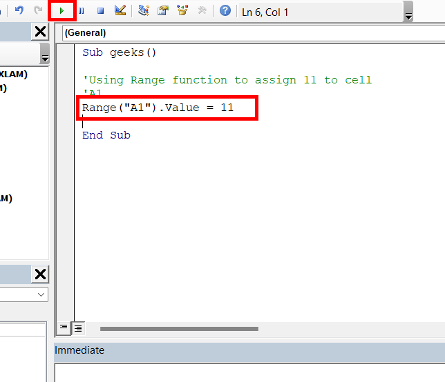
Step 2: Run your macro. The number 11 appears in cell A1.
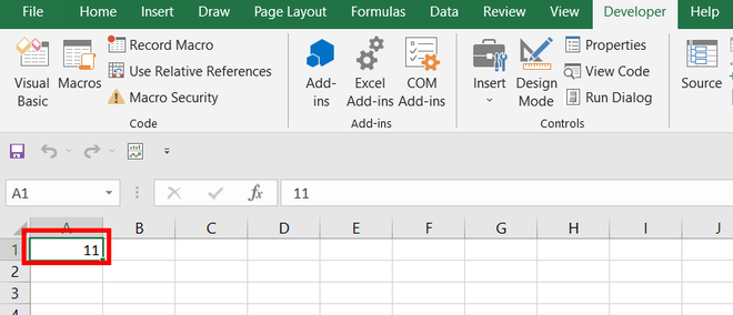
Set the value to multiple cells at the same time
Remember the days, when your teacher gives you punishment, by making you write the homework 10 times, those were the hard days, but now the effort has exponentially reduced. You can set a value to a range of cells with just one line of code. If you want to write your name, for example, “Arushi” 10 times, in the range A2 to A11. Use range function. Following are the steps:
Step 1: Use the Range function, in the double quotes, write “Start_of_cell: End_of_cell”. Use .Value object function. For example, Range(“A2:A11”).Value = “Arushi”.
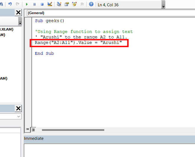
Step 2: Run your macro. The text “Arushi” appears from cell A2 to A11 inclusive.
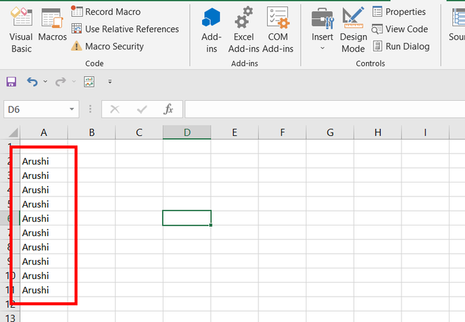
Cells Function in VBA
The Cells function is similar to the range function and is also used to set the cell value in a worksheet by VBA. The difference lies in the fact that the Cells function can only set a single cell value at a time while the Range function can set multiple values at a time. Cells function use matrix coordinate system to access cell elements. For example, A1 can be written as (1, 1), B1 can be written as (1, 2), etc.
Syntax: Cells(row_number, column_number).Value = value_to_be_assign
For example, you want to set the cell value to “Arushi cleared CA with Rank “, in cell B1. Also, set cell C1, to ‘1’. Following are the steps:
Step 1: Open your VBA editor. Use cells function, as we want to access cell B1, the matrix coordinates will be (1, 2). Type, Cells(1, 2).Value = “Arushi cleared CA with Rank” in the VBA code.
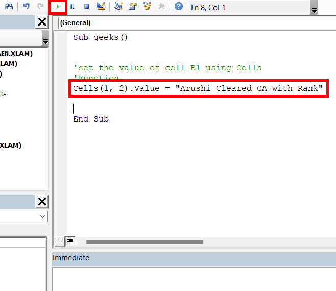
Step 2: To access cell C1, the matrix coordinates are (1, 3). Type, Cells(1, 3).Value = 1 in the VBA code.
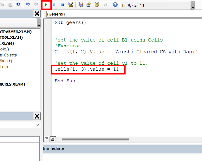
Step 3: Run your macro. The required text appears in cell B1, and a number appears in C1.
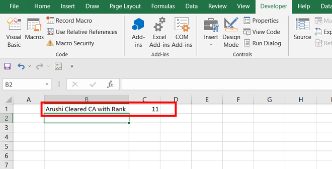
Setting Cell values by Active cell and the input box
There are other ways by which you can input your value in the cell in a worksheet.
Active Cell
You can set the cell value of a cell that is currently active. An active cell is the selected cell in which data is entered if you start typing. Use ActiveCell.Value object function to set the value either to text or to a number.
Syntax: ActiveCell.Value = value_to_be_assigned
For example, you want to assign the active cell with a text i.e. “Arushi is practicing CA”, also want to change the color of the cell to yellow. Following are the steps:
Step 1: Use the ActiveCell object to access the currently selected cell in the worksheet. Use ActiveCell.Value function object to write the required text.
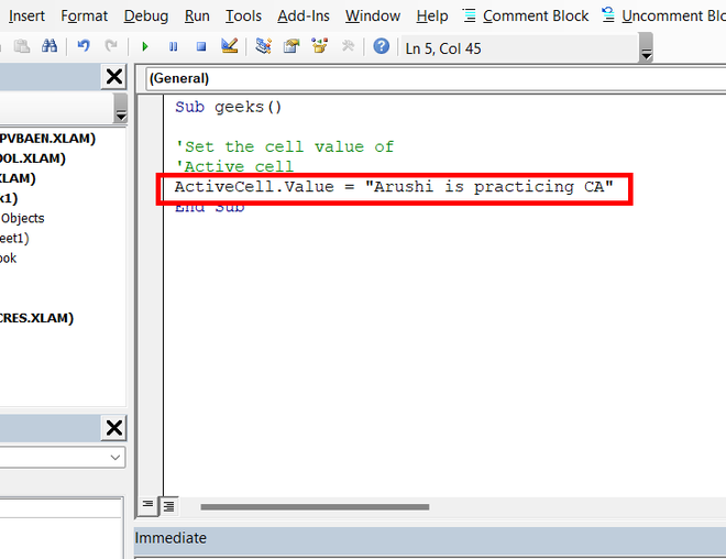
Step 2: Color the cell by using ActiveCell.Interior.Color function. For example, use vbYellow to set your cell color to yellow.
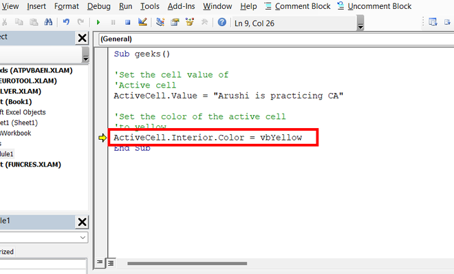
Step 3: Run your macro. The currently selected cell i.e. B1 has attained the requirements.
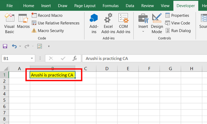
Input Box
You can use the input box to set the cell value in a worksheet. The input box takes the custom value and stores the result. This result could further be used to set the value of the cell. For example, set the cell value of A1, dynamically by taking input, from the input box.
Following are the steps
Step 1: Open your VBA editor. A sub-procedure name geeks() is created. Use the Range function to store the value given by the input box.
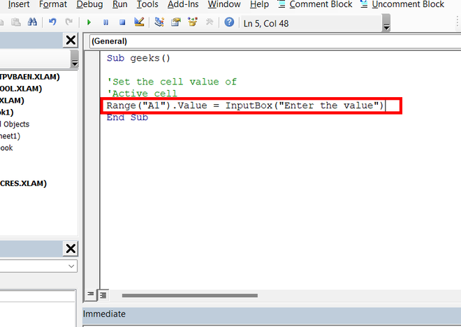
Step 2: Run your Macro. A dialogue-box name Microsoft Excel appears. Enter the value to be stored. For example, “geeks for geeks”. Click Ok.
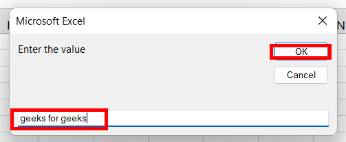
Step 3: Open your worksheet. In cell A1, you will find the required text is written.
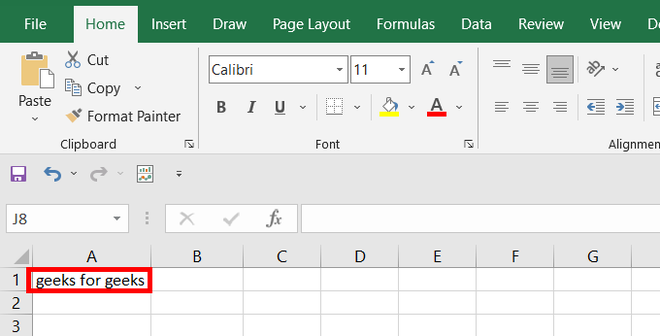
Get Cell Value
After setting the cell value, it’s very important to have a handsome knowledge of how to display the cell value. There can be two ways two get the cell value either print the value in the console or create a message box.
Print Cell Value in Console
The console of the VBA editor is the immediate window. The immediate window prints the desired result in the VBA editor itself. The cell value can be stored in a variable and then printed in the immediate window. For example, you are given a cell A1 with the value ’11’, and you need to print this value in the immediate window.
Following are the steps
Step 1: Press Ctrl + G to open the immediate window.
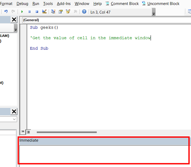
Step 2: The cell value in A1 is 1.
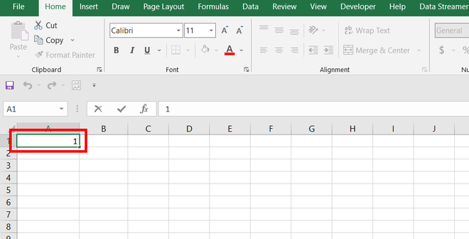
Step 3: Open your VBA editor. Declare a variable that could store the cell value. For example, Val is the variable that stores the cell value in A1. Use the Range function to access the cell value. After storing the cell value in the val, print the variable in the immediate window with the help of Debug.Print(val) function.
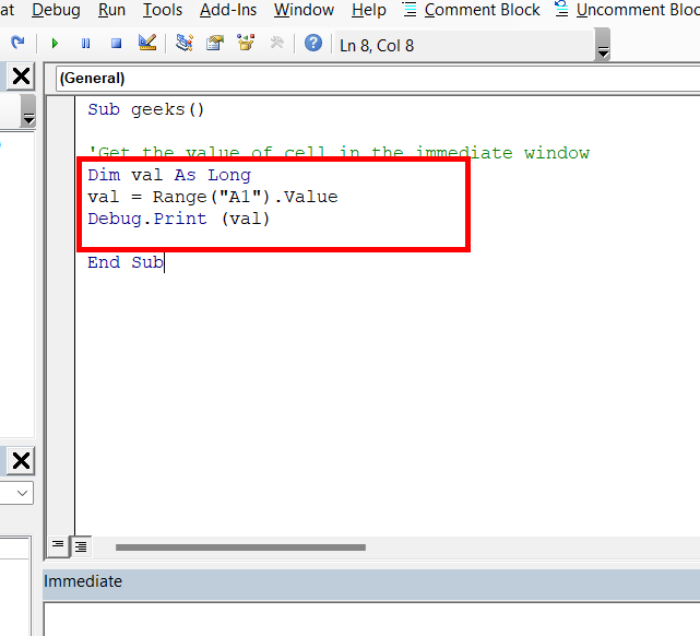
Step 4: Run your macro. The cell value in A1 is printed in the immediate window.
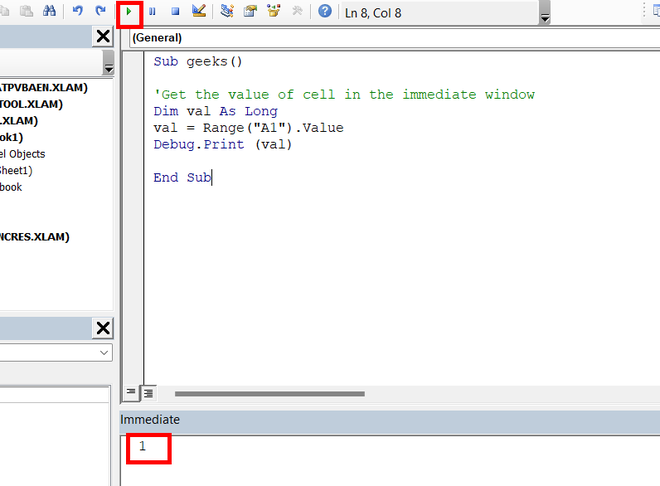
Print Cell Value in a Message Box
A message box can also be used to show the cell value in VBA. For example, a random string is given in cell A1 of your string i.e. “Arushi studies in Hansraj”. Now, if you want to display the cell value in A1, we can use Message Box to achieve this.
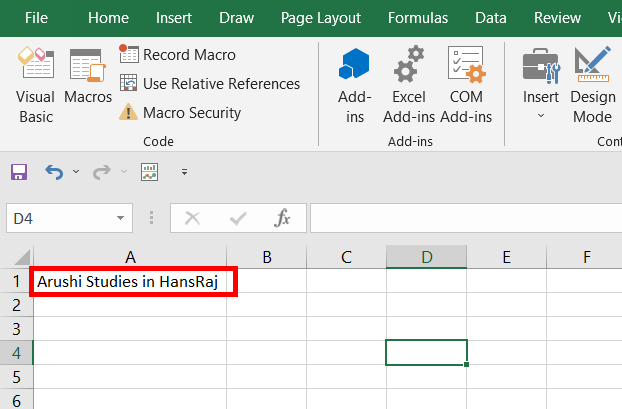
Following are the steps
Step 1: Open your VBA macro. Create a message box by using MsgBox. Use the Range(cell).Value function to access the cell value.
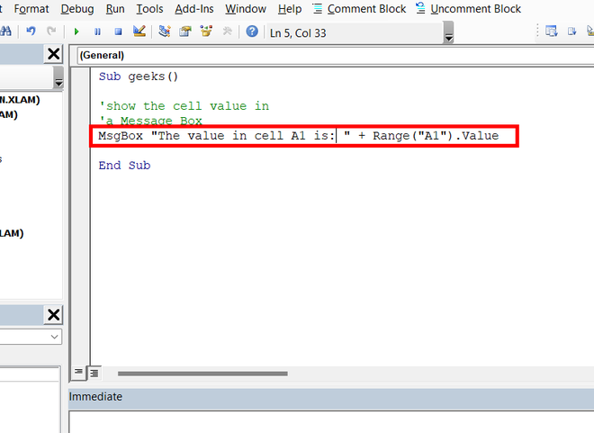
Step 2: Run your macro. A message box appears, which contains the cell value of A1.
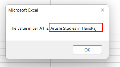
Change Cell Values
The value, once assigned to the cell value, can be changed. Cell values are like variables whose values can be changed any number of times. Either you can simply reassign the cell value or you can use different comparators to change the cell value according to a condition.
By reassigning the Cell Value
You can change the cell value by reassigning it. In the below example, the value of cell A1 is initially set to 1, but later it is reassigned to 2.
Following are the steps
Step 1: Open your VBA code editor. Initially, the value of cell A1 is assigned to 1. This initial value is printed in the immediate window. After that, we changed the value of cell A1 to 2. Now, if we print the A1 value in the immediate window, it comes out to be 2.
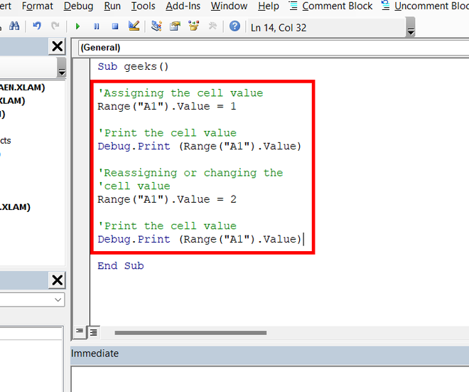
Step 2: The immediate window shows the output as 1 and 2.
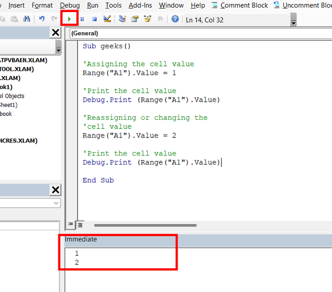
Changing cell value with some condition
We can use if-else or switch-case statements to change the cell value with some condition. For example, if your age is greater than 18 then you can drive else you cannot drive. You can output your message according to this condition.
Following are the steps
Step 1: A code is written in the image below, which tells whether you are eligible for a driving license or not. If your age is greater than 18 then cell A1 will be assigned with the value, “You are eligible for the driving license”, else A1 will be assigned with “You are not eligible for driving license”.
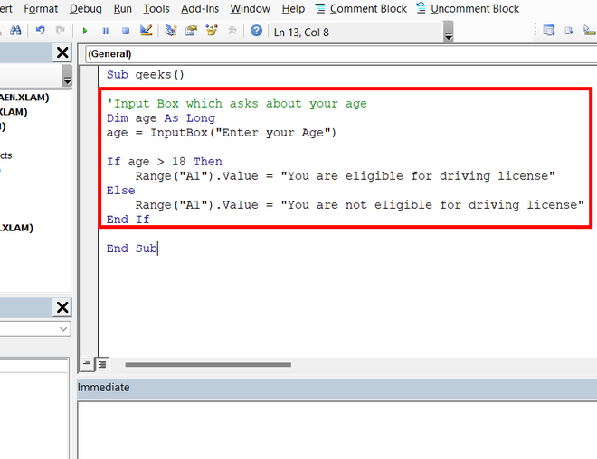
Step 2: Run your macro. An input box appears. Enter your age. For example, 19.
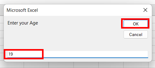
Step 3: According to the age added the cell value will be assigned.