Shapiro wilk test in excel - Word и Excel - помощь в работе с программами

This tutorial will demonstrate ho to perform the Shapiro-Wilk test in Excel and Google Sheets.

Shapiro-Wilk test is a statistical test conducted to determine whether a dataset can be modeled using the normal distribution, and thus, whether a randomly selected subset of the dataset can be said to be normally distributed. The Shapiro-Wilk test is considered one of the best among the numerical methods of testing for normality because of its high statistical power.

The original Shapiro-Wilk test, like most significance tests, is affected by the sample size and works best for sample sizes of n=2 to n=50. For larger sample sizes (up to n=2000), an extension of the Shapiro-Wilk test called the Shapiro-Wilk Royston test can be used.

How Shapiro-Wilk Test Works

The Shapiro-Wilk test tests the null hypothesis that the dataset comes from a normally distributed population against the alternative hypothesis that the dataset does not come from a normally distributed population.

The test statistics for the Shapiro-Wilk test is given as follows:

where x_(i) is the i^th order statistic (i.e. the i^thdata value after the dataset is arranged in ascending order),

is the mean (average) of the dataset.

n is the number of data points in the dataset, and

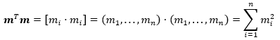
a = [a_i] = (a₁,…,a_n) is the coefficient vector of the weights of the Shapiro-Wilk test (obtained from the Shapiro-Wilk test table),

The vector a is anti-symmetric, that is a _n+1-i =-a_i for all i, and a_(n+1)/2 = 0 for odd n. Also, a^T a = 1.

The p-value is obtained by comparing the W statistic with the W values presented in the Shapiro-Wilk test table of p-values for the given sample size.

If the obtained -value is less than the chosen significance level, the null hypothesis is rejected, and it is concluded that the dataset is not from a normally distributed population,
Otherwise, the null hypothesis is not rejected and it is concluded that there is no statistically significant evidence that the dataset does not come from a normally distributed population.

How to Perform the Shapiro-Wilk Test in Excel

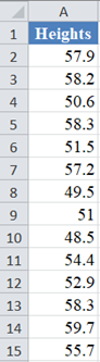
Background: A sample of the heights, in inches, of 14 ten years old boys are presented in the table below. Use the Shapiro-Wilk method of testing for normality to test whether the data obtained from the sample can be modeled using a normal distribution.

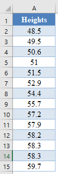
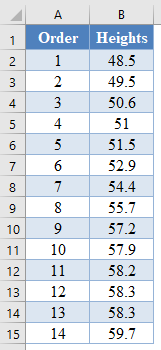
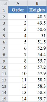
First, select the values in the dataset and Sort the data using the Sort tool: Data > Sort (Sort Smallest to Largest)

This will sort the values like so:

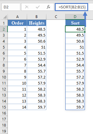
Alternatively, with newer versions of Excel, you can use the SORT Function to sort the data:

=SORT(B2:B15)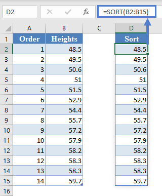

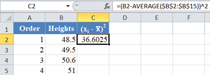
Sort

Next, calculate the denominator of the W statistic, , as shown in the picture below, using AVERAGE to calculate the mean:

=(B2-AVERAGE($B$2:$B$15))^2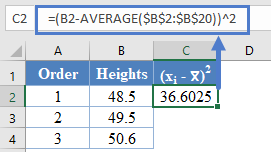

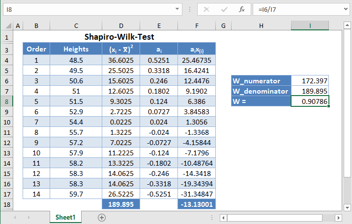
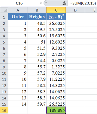
Complete the rest of the column and then calculate the sum (shown in green background) as shown in the picture below:

=SUM(C2:C15)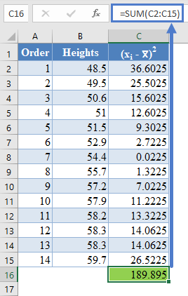

Thus, the denominator of the W statistic is 189.895.

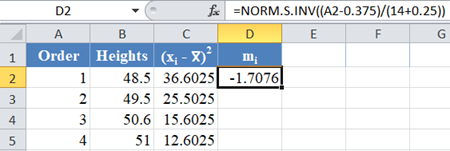
Next, obtain the values of a_i, the coefficients of the weights of the Shapiro-Wilk test, for a sample size of n=14 from the Shapiro-Wilk test table. An excerpt of the Shapiro-Wilk test table is shown below:

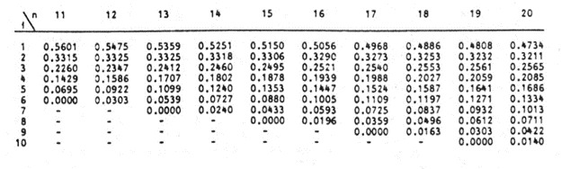
These values will need to be entered manually as follows:

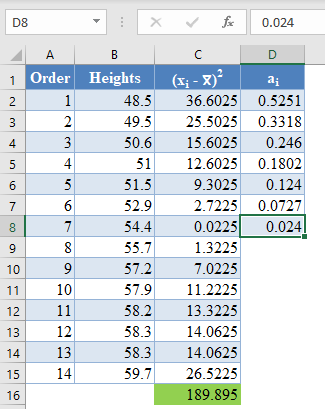
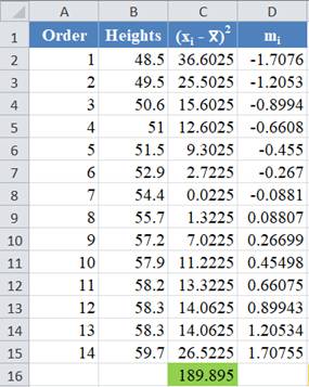
And using the anti-symmetric property of ai, that is, a_n+1-i=-a_i for all i, we have that a₁₄=-a₁, a₁₃=-a₂, etc. So, the complete values of the a_i column are shown in the picture below:

=-D8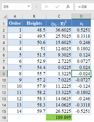

*Note that because of the anti-symmetric property of a_iand since that numerator of the W statistic is a square, it does not matter which half of the a_icolumn is positive or negative. That is, you can choose to make the upper half of the column to be positive and the lower half negative or vice-versa and it will not affect your final result.

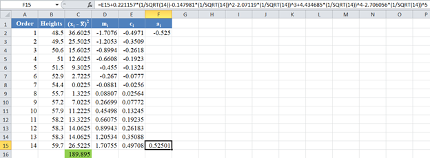
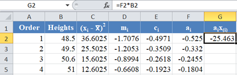
Next, multiply the a_i values with the corresponding (already arranged) values in the dataset to get the a_ix_(i) column. The calculation and the value for the first data point are shown in the picture below:

=D2*B2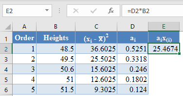

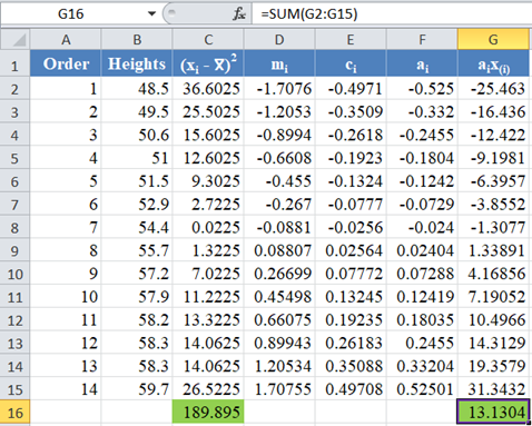
Complete the rest of the a_ix_(i) column and calculate the sum (shown in green background) as shown in the picture below:

=sum(E2:E15)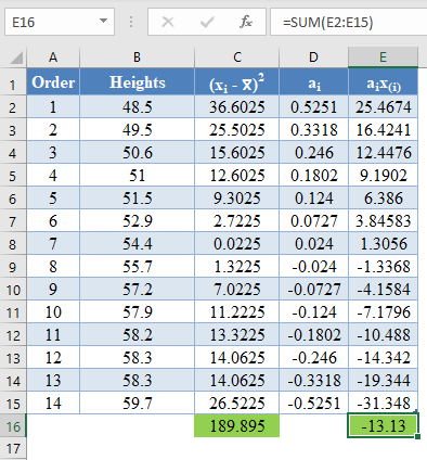

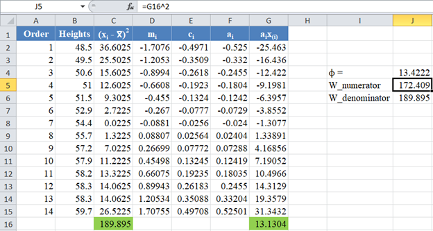
The denominator of the W statistic as obtained previously is 189.895 , and the numerator is the square of the sum of the a_ix_(i) column. Thus, we have as follows:

=E16^2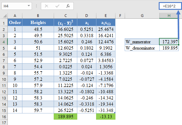

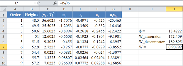
Therefore, the W statistic is as shown below:

=H4/H5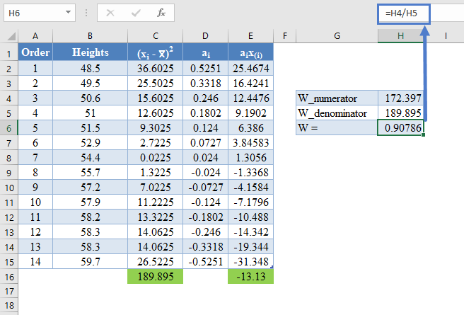

Finally, obtain the p-value of the test using the Shapiro-Wilk test table of p-values considering the sample size.

An excerpt of the Shapiro-Wilk test table of p-values is shown below:

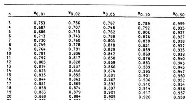
For this test, we will use a significance (alpha) level of 0.05. From the table, you can see that for n =14, W = 0.90786 is between W_0.10 = 0.895 and W_0.50 = 0.947, which means that the p-value is between 0.10 and 0.50. This means that the p-value is greater than α = 0.05, hence, the null hypothesis is not rejected.

Therefore, we conclude that there is not enough evidence that the dataset is not drawn from a normally distributed population. That is, we can assume that the dataset is normally distributed.

*Using linear interpolation, you can get that the approximate p-value is 0.1989.

Shapiro-Wilk Test in Google Sheets

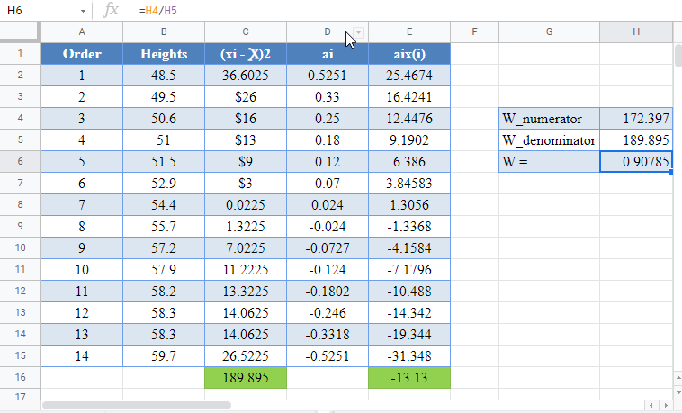
Shapiro-Wilk test can be conducted in Google Sheets in a similar way as done in Excel as shown in the picture below.

Источник

Содержание

Shapiro-Wilk Test Excel and Google Sheets
How Shapiro-Wilk Test Works
How to Perform the Shapiro-Wilk Test in Excel
Shapiro-Wilk Test in Google Sheets
Shapiro-Wilk Royston Test – Excel and Google Sheets
How the Shapiro-Wilk Royston Test Works
Royston’s Algorithm for the Approximation of a
The Shapiro-Wilk Royston Test’s Test Statistic
How to Perform the Shapiro-Wilk Royston Test in Excel
Shapiro-Wilk Royston Test in Google Sheets

Shapiro-Wilk Test Excel and Google Sheets

This tutorial will demonstrate ho to perform the Shapiro-Wilk test in Excel and Google Sheets.

How Shapiro-Wilk Test Works

The test statistics for the Shapiro-Wilk test is given as follows:

where x_(i) is the i th order statistic (i.e. the i th data value after the dataset is arranged in ascending order),

is the mean (average) of the dataset.

n is the number of data points in the dataset, and

a = [a_i] = (a₁,…,a_n ) is the coefficient vector of the weights of the Shapiro-Wilk test (obtained from the Shapiro-Wilk test table),

The vector a is anti-symmetric, that is a _n+1-i =-a_i for all i, and a_(n+1)/2 = 0 for odd n. Also, a T a = 1.

The p-value is obtained by comparing the W statistic with the W values presented in the Shapiro-Wilk test table of p-values for the given sample size.

If the obtained -value is less than the chosen significance level, the null hypothesis is rejected, and it is concluded that the dataset is not from a normally distributed population,
Otherwise, the null hypothesis is not rejected and it is concluded that there is no statistically significant evidence that the dataset does not come from a normally distributed population.

How to Perform the Shapiro-Wilk Test in Excel

First, select the values in the dataset and Sort the data using the Sort tool: Data > Sort (Sort Smallest to Largest)

This will sort the values like so:

Alternatively, with newer versions of Excel, you can use the SORT Function to sort the data:

Next, calculate the denominator of the W statistic, 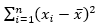, as shown in the picture below, using AVERAGE to calculate the mean:

Complete the rest of the column and then calculate the sum (shown in green background) as shown in the picture below:

Thus, the denominator of the W statistic is 189.895.

Next, obtain the values of a_i , the coefficients of the weights of the Shapiro-Wilk test, for a sample size of n=14 from the Shapiro-Wilk test table. An excerpt of the Shapiro-Wilk test table is shown below:

These values will need to be entered manually as follows:

And using the anti-symmetric property of ai, that is, a_n+1-i=-a_i for all i, we have that a₁₄=-a₁, a₁₃=-a₂, etc. So, the complete values of the a_i column are shown in the picture below:

*Note that because of the anti-symmetric property of a_i and since that numerator of the W statistic is a square, it does not matter which half of the a_i column is positive or negative. That is, you can choose to make the upper half of the column to be positive and the lower half negative or vice-versa and it will not affect your final result.

Next, multiply the a_i values with the corresponding (already arranged) values in the dataset to get the a_i x_(i) column. The calculation and the value for the first data point are shown in the picture below:

Complete the rest of the a_i x_(i) column and calculate the sum (shown in green background) as shown in the picture below:

The denominator of the W statistic as obtained previously is 189.895 , and the numerator is the square of the sum of the a_i x_(i) column. Thus, we have as follows:

Therefore, the W statistic is as shown below:

Finally, obtain the p-value of the test using the Shapiro-Wilk test table of p-values considering the sample size.

An excerpt of the Shapiro-Wilk test table of p-values is shown below:

Therefore, we conclude that there is not enough evidence that the dataset is not drawn from a normally distributed population. That is, we can assume that the dataset is normally distributed.

*Using linear interpolation, you can get that the approximate p-value is 0.1989.

Shapiro-Wilk Test in Google Sheets

Shapiro-Wilk test can be conducted in Google Sheets in a similar way as done in Excel as shown in the picture below.

Источник

Shapiro-Wilk Royston Test – Excel and Google Sheets

This tutorial will demonstrate how to use the Shapiro-Wilk Royston Test in Excel and Google Sheets.

This article examines the Shapiro-Wilk Royston test which is the more popular version of the Shapiro-Wilk test used by many popular statistical software packages. To learn more about how to perform the original Shapiro-Wilk test, see the Shapiro-Wilk test article.

How the Shapiro-Wilk Royston Test Works

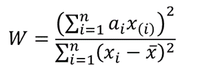
The W statistics for a Shapiro-Wilk Royston test is given as follows:

where x_(i) is the i th order statistic (i.e. the i th data value after the dataset is arranged in ascending order),

is the mean (average) of the dataset,

n is the number of data points in the dataset,

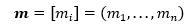
a=(a₁,…,a_n ) is the coefficient vector of the weights of the Shapiro-Wilk test representing the best linear estimate of the standard deviation of x_i, assuming normality, which we will approximate using Royston’s algorithm.

The vector a is anti-symmetric, that is a_(n+1-i) =-a_i for all i, and a_(n+1)/2 =0 for odd n. Also, .

Royston’s Algorithm for the Approximation of a

Royston’s algorithm for the approximation of a for the Shapiro-Wilk test starts with the fact that W statistics is asymptotically equivalent to the statistic, where 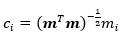, is the expectation vector of x_(i) with n standard normal random variables, 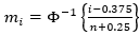, and Φ is the normal cdf.

Using the values above and setting , we have the following approximations for a_i:

Where: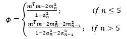

The Shapiro-Wilk Royston Test’s Test Statistic

For values of n between 4 and 11 , the statistic, w=-ln⁡[0.459n-2.273-ln⁡(1-W) ] , can be modeled with normal distribution with a mean, μ=0.544-0.39978n+0.062767n 2 -0.0020322n 3 and a standard deviation,

σ = exp(1.3822-0.77857n+0.062767n 2 -0.0020322n 3 )

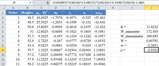
Similarly, for values of n between 12 and 2000, the statistic, w = ln(1-W), is normally distributed with a mean,

μ = 0.0038915x 3 – 0.083751x 2 – 0.31082x – 1.5861, and a standard deviation,

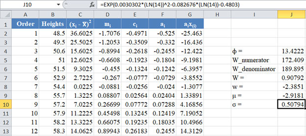
σ = exp(0.0030302x 2 – 0.082676x – 0.4803), where x = ln n.

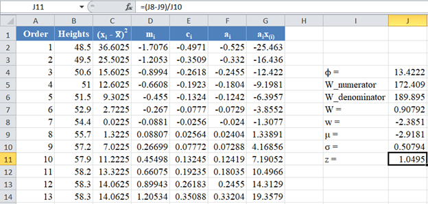
Thus, for the Shapiro-Wilk Royston test, the z-statistic is used as the test statistic and is given by

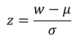
To find the p-value of the test, the z-score obtained above refers to the upper (right) tail of the standard normal curve.

If the obtained p-value is less than the chosen significant (alpha) level, the null hypothesis is rejected, and it is concluded that the dataset is not from a normally distributed population, otherwise, the null hypothesis is not rejected and it is concluded that there is no statistically significant evidence that the dataset does not come from a normally distributed population.

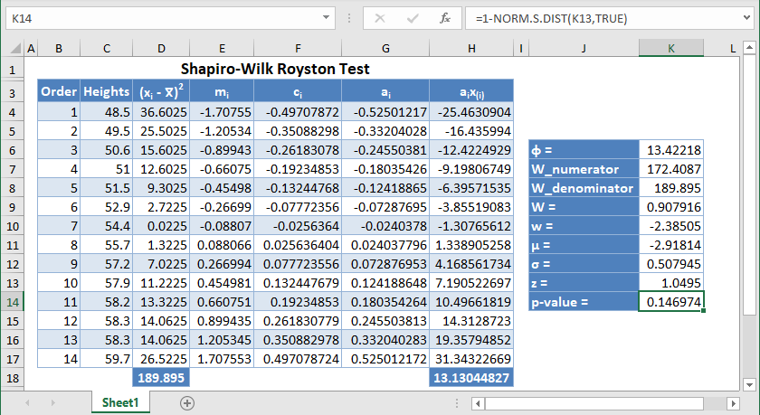
How to Perform the Shapiro-Wilk Royston Test in Excel

Background: A sample of the heights, in inches, of 14 ten years old boys are presented in the table below. Use the Shapiro-Wilk Royston method of testing for normality to test whether the data obtained from the sample can be modeled using a normal distribution.

First, select the values in the dataset and Sort the data: Data > Sort (Sort Smallest to Largest) to arrange the values in ascending order as shown below:

And the arranged values are as follows:

Alternatively, with newer versions of Excel, you can use the SORT Function to sort the data:

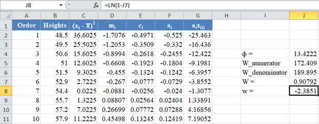
Next, calculate the W denominator of the statistic, , as shown in the picture below:

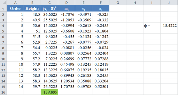
Complete the rest of the column and then calculate the sum (shown in green background) as shown in the picture below:

Thus, the denominator of the W statistic is 189.895.

Next, obtain the values of using the NORM.S.INV Function with the formula:

The formula and the value of m₁ are shown in the picture below:

*Note that for our case, n = 14 because we have 14 data points.

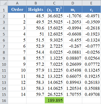
Complete the rest of the column as shown in the picture below:

Now, since is a column vector, then it follows that.

Thus, the value of 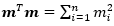can be calculated in Excel using the SUMSQ Function.

Thus, calculate the values of c_i using the formula:

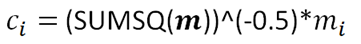
The formula for the value of C₁ is shown in the picture below:

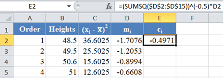
Complete the rest of the column as shown in the picture below:

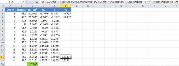
Next, use the formula given above to calculate the values of a_n and a_(n-1) for n=14, and because of the anti-symmetric property of a_i , a_n+1-i = – a_i . That is, a₁₄ = a₁ , a₁₃ = a₂, etc.

The formula and values of a₁₄ and a₁ are shown in the picture below:

Similarly, the formula and values of a₁₃ and a₂ are shown in the picture below:

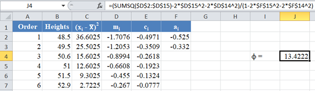
Next, obtain the value of 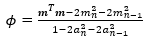, noting that, as established above, 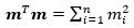. The formula and the value of ϕ are shown in the picture below:

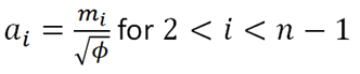
Then, using the value of ϕ, obtain the values of the rest of the a_i column using the formula: 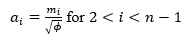for . The picture below shows the formula and value of a_{3 :}

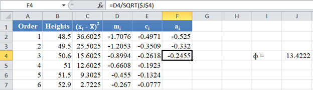
Thus, the complete values of the a_i column are shown in the picture below:

Next, multiply the a_i values with the corresponding (already arranged) values in the dataset to get the a_i x_(i)

column. The calculation and the value for the first data point are shown in the picture below:

Complete the rest of the a_i x_(i) column and calculate the sum (shown in green background) as shown in the picture below:

The denominator of the W statistic as obtained previously is 189.895 , and the numerator is the square of the sum of the a_i x_(i) column. Thus, we have as follows:

Therefore, the W statistic is as shown below:

*Note that the value of the W statistic will always be between 0 and 1.

Next, obtain the values of the w statistic, μ and σ using the formulas stated previously in this article.
For our case, n=14, so we use the formula w=ln⁡(1-W) as shown in the picture below:

Calculate the value of μ as shown in the picture below:

Also, calculate the value of σ as shown in the picture below:

Next, obtain the z-score using the formula stated previously as shown in the picture below:

Finally, obtain the p-value using the NORM.S.DIST Function.

Since the p-value of the Shapiro-Wilk Royston test is the upper tail of the standard normal curve, we used the formula: p-value 1 – NORM.S.DIST(z, TRUE) to obtain the p-value as shown in the picture below:

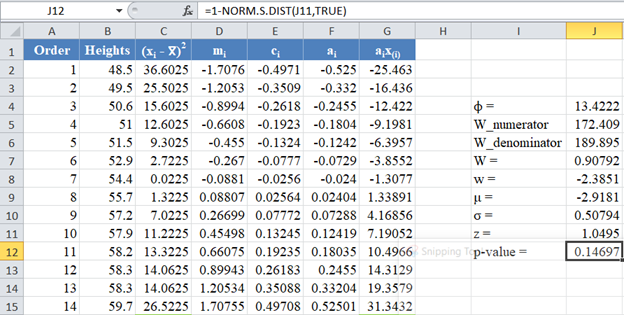
The p-value is 0.14697, which is greater than α=0.05, hence, the null hypothesis is not rejected.

Therefore, we conclude that there is not enough evidence that the dataset is not drawn from a normally distributed population. That is, we can assume that the dataset is normally distributed.

Shapiro-Wilk Royston Test in Google Sheets

Shapiro-Wilk Royston test can be conducted in Google Sheets in a similar way as done in Excel as shown in the picture below.

Источник

Why do we need to run a normality test?

Normality tests enable you to know whether your dataset follows a normal distribution. Moreover, normality of residuals is a required assumption in common statistical modeling methods.
Normality tests involve the null hypothesis that the variable from which the sample is drawn follows a normal distribution. Thus, a low p-value indicates a low risk of being wrong when stating that the data are not normal. In other words, if p-value < alpha risk threshold, the data are significantly not normal.

How do normality tests work?

We calculate the test statistic below on our dataset :

W=(∑i=1naix(i))2∑i=1n(xi−xˉ)2W=dfrac{(sum_{i=1}^na_ix_{(i)})^2}{sum_{i=1}^n(x_i-bar{x})^2}

If its values are below the bounds defined in the Shapiro-Wilk table for a set alpha threshold, then the associated p-value is less than alpha and the null hypothesis is rejected and the data does not follow a normal distribution.

Dataset for Shapiro-Wilk and other normality tests

The data represent two samples each containing the average math score of 1000 students.

Setting up a Shapiro-Wilk and other normality tests

We then want to test the normality of the two samples. Select the XLSTAT / Describing data / Normality tests, or click on the corresponding button of the Describing data menu.

Once you’ve clicked on the button, the dialog box appears. Select the two samples in the Data field.
The Q-Q plot option is activated to allow us to visually check the normality of the samples.

The computations begin once you have clicked on the OK button, and the results are displayed on a new sheet.

Interpreting the results of a Shapiro-Wilk and other normality tests

The results are first displayed for the first sample and then for the second sample.
The first result displayed is the Q-Q plot for the first sample. The Q-Q plot allows us to compare the cumulative distribution function (cdf) of the sample (abscissa) to the cumulative distribution function of the normal distribution with the same mean and standard deviation (ordinates). In the case of a sample following a normal distribution, we should observe an alignment with the first bisecting line. In the other cases some deviations from the bisecting line should be observed.
QQ plot
We can see here that the empiric cdf is very close to the bisecting line. The Shapiro-Wilk and Jarque-Bera confirm that we cannot reject the normality assumption for the sample. We notice that with the Shapiro-Wilk test, the risk of being wrong when rejecting the null assumption is smaller than with the Jarque-Bera test.

The following results are for the second sample. Contrary to what we have observed for the first sample, we notice here on the Q-Q plot that there are two strong deviations indicating that the distribution is most probably not normal.

This gap is confirmed by the normality tests (see below) which allow us to assert with no hesitation that we need to reject the hypothesis that the sample might be normally distributed.

Conclusion

In conclusion, in this tutorial, we have seen how to test two samples for normality using Shapiro-Wilk and Jarque-Bera tests. These tests did not reject the normality assumption for the first sample and allowed us to reject it for the second sample.

Was this article useful?

Источник

The purpose of this blog article is to show how to create a completely automated Shapiro-Wilk test for normality in Excel. The test is completely automated because the user has only to enter the raw, unsorted data sample to be tested for normality along with the alpha level desired for the test. Upon insertion of the sample data and alpha, the entire test will be automatically run and the test’s output will be immediately returned.

As with any hypothesis test, the output states whether to reject or not reject the Null Hypothesis and the specified alpha level. In this case, the Null Hypothesis states that the data sample came from a normally distributed population. This Null Hypothesis is rejected only if Test Statistic W is less than the critical value of W for a given alpha level and sample size.

Overview of the Shapiro-Wilk Test For Normality

The Shapiro-Wilk Test is a hypothesis test that is widely used to determine whether a data sample is normally distributed. A test statistic W is calculated. If this test statistic is less than a critical value of W for a given level of significance (alpha) and sample size, the Null Hypothesis which states that the sample comes from a normally distributed population is rejected. Keep in mind that passing a hypothesis test for normality only allows one to state that no significant departure from normality was found.

The Shapiro-Wilk Test is a robust normality test and is widely-used because of its slightly superior performance against other normality tests, especially with small sample sizes. Superior performance means that it correctly rejects the Null Hypothesis that the data are not normally distributed a slightly higher percentage of times than most other normality tests, particularly at small sample sizes.

The Shapiro-Wilk normality test is generally regarded as being slightly more powerful than the Anderson-Darling normality test, which in turn is regarded as being slightly more powerful than the Kolmogorov-Smirnov normality test. The Shapiro-Wilk normality test is affected by tied data values but less so than the Anderson-Darling normality test.

An abbreviated description of the steps of the Shapiro-Wilk normality test is as follows:

Sort the raw data in an ascending sort
Arrange the sorted data into pairs of successive highest and lowest data values
Calculate the difference between the high and low value of each pair
Multiply each difference by an “a Value” from a lookup table
Calculate test statistic W
Compare test statistic W with a W Critical Value obtained from a lookup table
Reject the Null Hypothesis stating normality only if W is smaller than W Critical

The complete Shapiro-Wilk test of normality appears in Excel as follows:

(Click On Image To See a Larger Version)

Step 1 – Sort Data in an Ascending Sort

Enter the Raw Data and Alpha Level

First, paste in the raw, unsorted data and set the alpha level in the yellow cells as follows:

(Click On Image To See a Larger Version)

This Shapiro-Wilk normality test in Excel has the capability to handle up to 20 data points. This data sample contains only 15 data points but the Excel worksheet below indicates the capability for an additional 5 data points in the empty yellow cells. Expanding the capability of this Excel test to handle a larger number of data points would be a straightforward matter of making adjustments to the Excel formulas.

The alpha level should be set at 0.01, 0.05, or 0.10 because critical values of W are provided here only for those common alpha levels. If alpha is set at a different level, the following warning appears as a result of the If-Then-Else statement seen in the previous image:

(Click On Image To See a Larger Version)

Sort the Raw Data Using Formulas, Not the Excel Sorting Tool

The most efficient way to sort data is with the use of formulas as shown. The Excel sorting tool must be manually re-run whenever the raw data is changed in any way. The following formula will automatically resort the data if any data are changed or added. The following formulas produce an ascending sort. To create a descending sort, simply swap the word LARGE for SMALL within the formula.

(Click On Image To See a Larger Version)

Step 2 – Obtain “a Values” From the “a Value Lookup Table”

The Table of a Values

The a Values are constants that are calculated from the means, variances, and covariances of the order statistics of a sample of size n from a normal distribution. The a Value table is shown as follows for data samples varying in size from n = 2 up to n = 50.

(Click On Image To See a Larger Version)

Create Labels for the a Values

The first step in obtaining the correct a Values is to create the proper number of labels for the a Values.

The number of a Values needed depends on the sample size n. If n is an even number, the number of a Values equals n / 2. If n is an odd number, the number of a Values equals (n-1) / 2. This can be implemented with the following formulas:

(Click On Image To See a Larger Version)

Lookup a Values on the a Value Lookup Table

The a Values can now be looked up on the a Value table previously shown. An Index formula is a straightforward way implementing this. The Excel Index function is its simplest form has the following format:

Index(array, row number, column number) and returns the data value located in the specified row and column of the given array. The row and column number are relative to the cell in the upper-left corner of the array. Note that the array containing the a Values starts in cell H58 at the upper left corner and finishes in cell BE82 in the lower right corner.

(Click On Image To See a Larger Version)

Step 3 – Pair Up Successive Highest-Lowest Data Values

Create X Labels for Data Sample Values

Each sorted data sample value will have an X Label. This is implemented with the following formulas:

(Click On Image To See a Larger Version)

The following is a close-up of the formulas to create the labels for the X Values:

(Click On Image To See a Larger Version)

The X Values are then obtained using the following formulas:

(Click On Image To See a Larger Version)

Create the Upper Value of Each Data Pair

The labels for the upper X Values of each data pair are created as follows:

The following is a close-up of the formulas to create the labels for the upper X Values:

(Click On Image To See a Larger Version)

The upper X Values of each data pair are the obtained using the following set of formulas:

(Click On Image To See a Larger Version)

Here is a close-up of those formulas:

(Click On Image To See a Larger Version)

Create the Lower Value of Each Data Pair

The labels for the lower X Values of each data pair are created as follows:

(Click On Image To See a Larger Version)

The following is a close-up of the formulas to create the labels for the lower X Values:

(Click On Image To See a Larger Version)

The lower X Values of each data pair are the obtained using the following set of formulas:

(Click On Image To See a Larger Version)

Here is a close-up of those formulas:

(Click On Image To See a Larger Version)

Step 4 – Calculate the Difference Within Each Pair

(Click On Image To See a Larger Version)

Here is a close-up of the difference formulas:

(Click On Image To See a Larger Version)

Step 5 – Calculate a * Difference

(Click On Image To See a Larger Version)

Here is a close-up of those formulas:

(Click On Image To See a Larger Version)

Step 6 – Calculate b, SS, and Test Statistic W

b equals the sums of the product of a * pair difference.

SS is the sum of the squared deviations of x from the mean x. Excel formula DEVSQ() performs this.

Test Statistic W equals b²/SS.

(Click On Image To See a Larger Version)

Here is a close-up of these formulas:

(Click On Image To See a Larger Version)

Step 7 – Lookup W Critical Values

Each unique combination of sample size and alpha level has its own critical W value. The following is a table of the respective critical W value for each combination of n and alpha up to a sample size of 50 and 3 common levels of alpha.

(Click On Image To See a Larger Version)

Here is a close-up of the formulas. The If-Then-Else statement that looks up the critical W value is the following:

=IF(OR(B1=0.01,B1=0.05,B1=0.1),INDEX(BL18:BN67,U14,IF(U12=0.01,1,IF(U12=0.05,2,IF(U12=0.1,3)))),”alpha must be set to 0.01, 0.05, or 0.10”)

The INDEX() function looks up the critical W values in the array starting in cell BL18 in the upper left corner and ending in cell BN67 in the lower right corner.

(Click On Image To See a Larger Version)

Step 8 – Determine Whether or Not To Reject Null Hypothesis By Comparing W to W Critical

The Null Hypothesis is rejected only if Test Statistic W is smaller the critical W value for the given sample size and alpha level. The Null Hypothesis states that the sample came from a normally distributed population. The Null Hypothesis is never accepted but only rejected or not rejected. Not rejecting the Null Hypothesis does not automatically imply that the population from which the sample was taken is normally distributed. This merely indicates that there is not even evidence to state that the population is likely not normally distributed for the given alpha level. As with all hypothesis tests, alpha = 1 — level of certainty. If a 95-percent level of certainty is required to reject the Null Hypothesis, the alpha level will be 0.05.

(Click On Image To See a Larger Version)

Here is a close-up of the formulas to compare W with W Critical:

(Click On Image To See a Larger Version)

The complete Shapiro-Wilk test of normality appears in Excel as follows:

(Click On Image To See a Larger Version)

Excel Master Series Blog Directory

Click Here To See a List Of All

Statistical Topics And Articles In

This Blog

You Will Become an Excel Statistical Master!

Источник

Тест Шапиро-Уилка является тестом на нормальность. Он используется для определения того, соответствует ли выборка нормальному распределению .

Этот тип теста полезен для определения того, исходит ли данный набор данных из нормального распределения, что является распространенным предположением, используемым во многих статистических тестах, включая регрессию , дисперсионный анализ , t-тесты и многие другие.

Мы можем легко выполнить тест Шапиро-Уилка для данного набора данных, используя следующую встроенную функцию в R:

Шапиро.тест(х)

куда:

x: числовой вектор значений данных.

Эта функция создает тестовую статистику W вместе с соответствующим p-значением. Если p-значение меньше, чем α = 0,05, имеется достаточно доказательств, чтобы сказать, что выборка не происходит из населения с нормальным распределением.

Примечание. Размер выборки должен быть от 3 до 5000, чтобы можно было использовать функцию shapiro.test().

В этом руководстве показано несколько примеров использования этой функции на практике.

Пример 1. Критерий Шапиро-Уилка для нормальных данных

В следующем коде показано, как выполнить тест Шапиро-Уилка для набора данных с размером выборки n = 100:

#make this example reproducible
set.seed(0)

#create dataset of 100 random values generated from a normal distribution
data <- rnorm(100)

#perform Shapiro-Wilk test for normality
shapiro.test(data)

 Shapiro-Wilk normality test

data: data
W = 0.98957, p-value = 0.6303

Значение p теста оказывается равным 0,6303.Поскольку это значение не меньше 0,05, мы можем предположить, что данные выборки получены из населения с нормальным распределением.

Этот результат не должен вызывать удивления, поскольку мы сгенерировали выборочные данные с помощью функции rnorm(), которая генерирует случайные значения из нормального распределения со средним значением = 0 и стандартным отклонением = 1.

Связанный: Руководство по dnorm, pnorm, qnorm и rnorm в R

Мы также можем создать гистограмму, чтобы визуально убедиться, что данные выборки распределены нормально:

hist(data, col='steelblue')

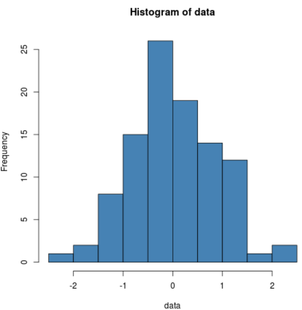
Мы видим, что распределение имеет довольно колоколообразную форму с одним пиком в центре распределения, что типично для данных с нормальным распределением.

Пример 2: тест Шапиро-Уилка на ненормальных данных

В следующем коде показано, как выполнить тест Шапиро-Уилка для набора данных с размером выборки n = 100, в котором значения генерируются случайным образом израспределения Пуассона :

#make this example reproducible
set.seed(0)

#create dataset of 100 random values generated from a Poisson distribution
data <- rpois(n=100, lambda=3)

#perform Shapiro-Wilk test for normality
shapiro.test(data)

 Shapiro-Wilk normality test

data: data
W = 0.94397, p-value = 0.0003393

Значение p теста оказывается равным 0,0003393.Поскольку это значение меньше 0,05, у нас есть достаточно доказательств, чтобы сказать, что данные выборки не получены из населения с нормальным распределением.

Этот результат не должен вызывать удивления, поскольку мы сгенерировали выборочные данные с помощью функции rpois(), которая генерирует случайные значения из распределения Пуассона.

Связанный: Руководство по dpois, ppois, qpois и rpois в R

Мы также можем создать гистограмму, чтобы визуально увидеть, что выборочные данные не распределены нормально:

hist(data, col='coral2')

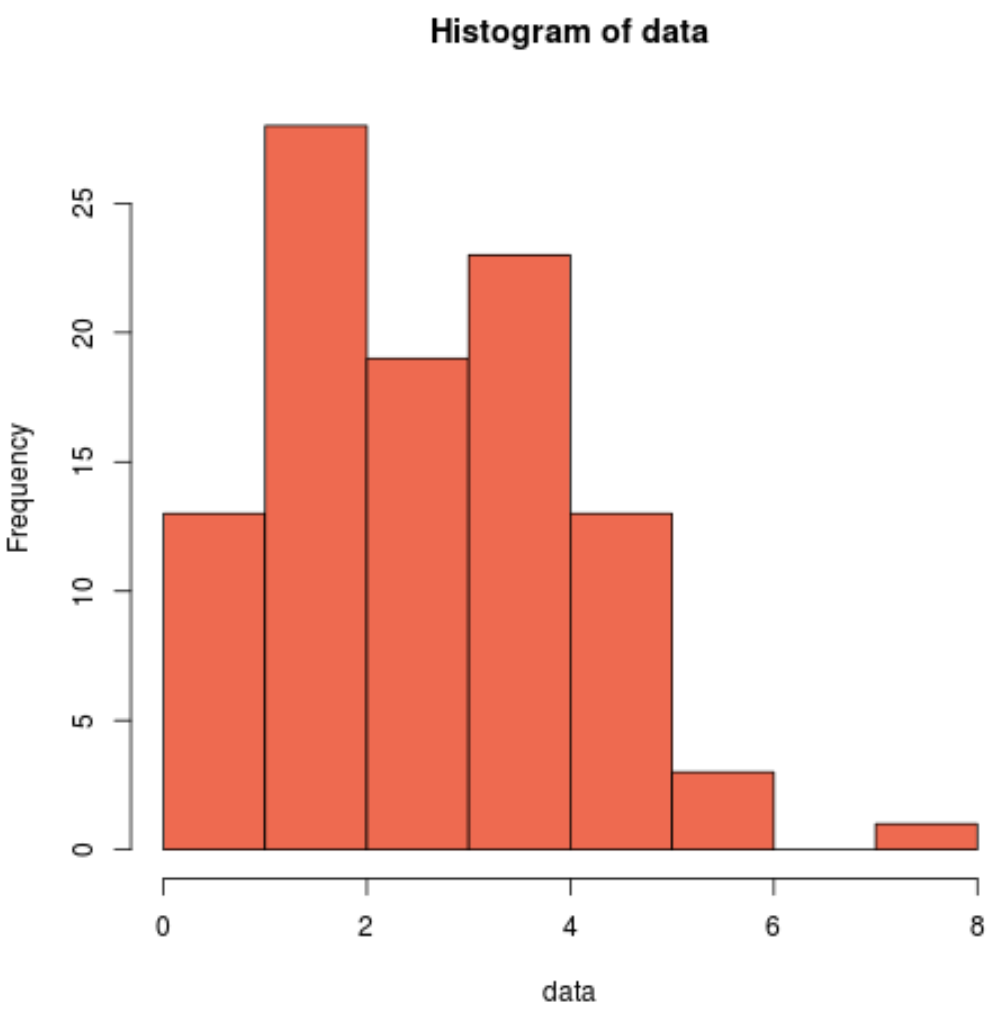
Мы видим, что распределение скошено вправо и не имеет типичной «колокольчатой формы», связанной с нормальным распределением. Таким образом, наша гистограмма соответствует результатам теста Шапиро-Уилка и подтверждает, что данные нашей выборки не имеют нормального распределения.

Что делать с ненормальными данными

Если данный набор данных не распределен нормально, мы часто можем выполнить одно из следующих преобразований, чтобы сделать его более нормальным:

1. Преобразование журнала: преобразование переменной ответа из y в log(y) .

2. Преобразование квадратного корня: преобразовать переменную отклика из y в √y .

3. Преобразование кубического корня: преобразовать переменную ответа из y в y 1/3 .

Выполняя эти преобразования, переменная отклика обычно становится ближе к нормально распределенной.

Ознакомьтесь с этим руководством , чтобы увидеть, как выполнять эти преобразования на практике.

Дополнительные ресурсы

Как провести тест Андерсона-Дарлинга в R
Как провести тест Колмогорова-Смирнова в R
Как выполнить тест Шапиро-Уилка в Python

Источник