Shapes in cells excel

To insert the cell content to your shape, do the following:

   1.   Select the shape or text box.

   2.   In the formula bar, type the equal («=«) symbol.

   3.   Click the spreadsheet cell that contains the data or text you want to
insert into the selected shape or text box.

You can also type the reference to the spreadsheet cell. Include the sheet name, for example:

= [officetooltips.xls]Tips!$B$2

   4.   Press Enter.

See also this tip in French:
Comment insérer le contenu de la cellule à la forme.

Please, disable AdBlock and reload the page to continue

Today, 30% of our visitors use Ad-Block to block ads.We understand your pain with ads, but without ads, we won’t be able to provide you with free content soon. If you need our content for work or study, please support our efforts and disable AdBlock for our site. As you will see, we have a lot of helpful information to share.

• #2

On your Drawing toolbar, goto Draw. There are many options for aligning autoshapes in there.

• #3

Objects in XL do not fit into a cell; instead, they ‘float’ in a layer above the cells layer. Consequently, it is not possible — without an incredible amount of work — to make an object appear as though it is part of the text within a cell.

That said, XL does support some rudimentary shape position and size relative to the underlying cell. Double click the object and select the Properties tab.

gnaga said:

I would like to draw a shape (for ex. Smily Face) in a cell and want to align with the cell like formating a text in the cell. Horizontally and vertically center and if cell changes this (shape) also shoud get adjust it to the cell size. Is this possible?

• #4

Thanks for both of you.

In Draw option in the drawing toolbar has some options for aligning the shape but it is not gettting enabled even I select the shape object. I do not know how to make them enable.

Tushar, If I copy & paste an exisiting shape, it is not getting pasted into my deisred location but close to the copied shape. How to move this shape object into a desired location in the worksheet?

• #5

For a shape taken created by using the Excel Drawing toolbar, or for an image or picture that has been pasted, click on top of the shape or picture. You should see the eight little sizing squares, and the cursor turns into a four-arrow shape. Just click and hold down the left mouse button, and drag the shape where you want it, then, release the mouse button. That’s it!

• #6

Ralph Thanks. I am aware of the technique you have suggested. I wanted to copy the shape or image and then I want to paste it in a location thorugh VBA. Is the worksheet has any dimension based on pixels to place the image into a particular location?

• #7

Code:

Sub testIt()
    With ActiveSheet.Shapes(1)
    .Height = .Height / 2
    .Width = .Width / 2
    .Left = Range("c1").Left
    .Top = Range("c1").Top
        End With
    End Sub

• #8

Tushar Thank you very much. This is the one I was looking for. Now I can manipulate with this to complete my work.

• #9

Code:

Sub testIt()
    With ActiveSheet.Shapes(1)
    .Height = .Height / 2
    .Width = .Width / 2
    .Left = Range("c1").Left
    .Top = Range("c1").Top
        End With
    End Sub

Perfect! this is also just what I needed, Tusharm, thank you!

In this article, you will learn how to make a circle around something in Excel and Google Sheets.

Make a Circle Around a Cell

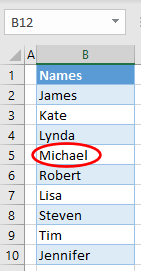
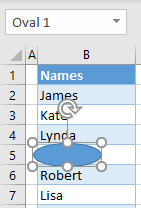
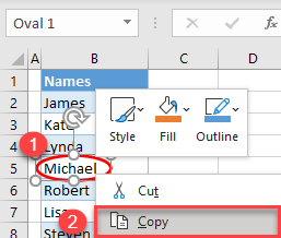
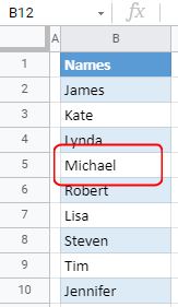
In Excel, you can circle a cell using the oval shape. Say you have the following list of names in Column B:

You can circle, for example, Michael in cell B5 with a red oval.

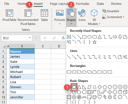
1. In the Ribbon, go to Insert > Shapes > Basic Shapes > Oval. Here you can choose to insert any shape offered (rectangle, circle, etc.). Any shape that you insert will be added to the Recently Used Shapes section at the top.

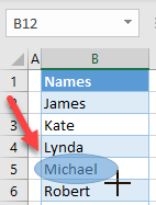
2. A small black cross appears. Position it where you want to start the shape and drag the cursor to form the shape.

As a result of this step, the oval is inserted, but as you can see below, the fill color and line color are both blue. The shape needs to have a red line and transparent fill, so you can see the text from the cell underneath.

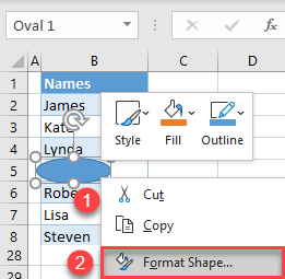
3. To change the oval’s appearance, right-click on the shape and choose Format Shape.

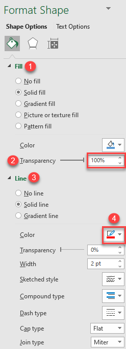
4. The Format Shape menu comes up on the right side of the screen. (1) Click Fill, and (2) set the transparency to 100% (this removes the fill color of the shape). Then (3) click Line, and (4) choose the line color (red).

Finally, the shape is transparent with the red outline, and the text in B5 is circled. Similarly, you can also circle a range of cells by expanding the shape.

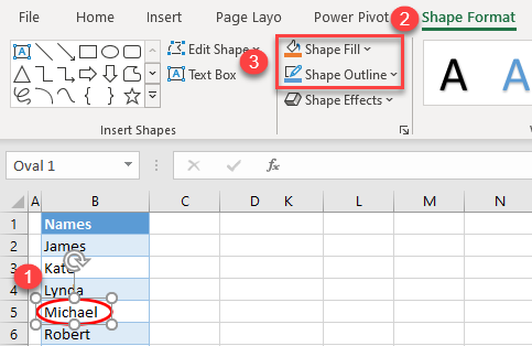
Another option to format the shape is to use the options in the Ribbon. To do this, click on the shape to select it, and in the Ribbon, go to Format Shape > Shape Fill (and Shape Outline).

Note: You can also insert a shape using VBA code.

Copy a Circle

Now let’s say you want to circle another name (for example, Jennifer) with the same shape (transparent with a red outline). To avoid formatting a new shape, you can copy the existing one and position it around cell B10.

1. Right-click the shape, and choose Copy (or use the keyboard shortcut CTRL + C).

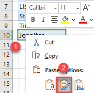
2. Right-click the cell where you want to paste the shape (B10), and choose Paste (Keep source formatting, or use the keyboard shortcut CTRL + V).

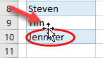
3. Now the shape is in the right general area, but it is not positioned ideally around the text in the cell. Therefore, you have to move it a bit. To do this, position the cursor on the shape, and when the four-sided arrow appears, drag and drop the shape.

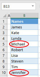
As a result, you have a new shape copied from the original one.

Make a Circle Around a Cell in Google Sheets

You can also add a shape to circle a cell in Google Sheets.

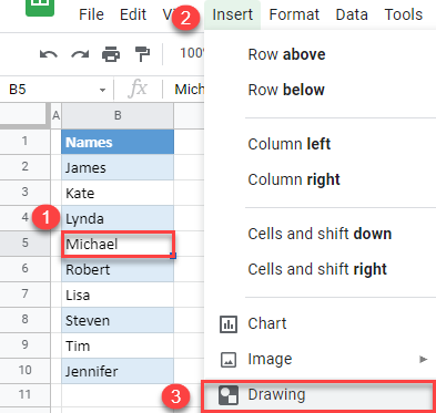
1. Select a cell where you want to add a circle (B5) and in the menu, go to Insert > Drawing.

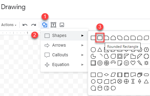
2. In the Drawing window, (1) click the shape icon, then (2) select Shapes and (3) choose a shape (e.g., Rounded Rectangle).

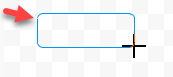
3. A black cross appears. Position it where you want to start your shape and drag the cursor to form the shape.

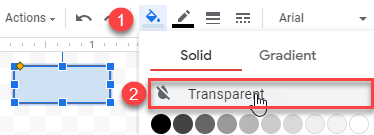
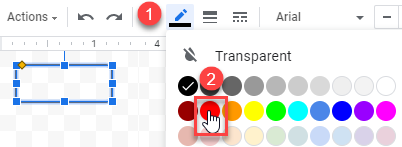
4. Click the fill color icon, and choose Transparent.

5. Click the border color icon, and select the color (red).

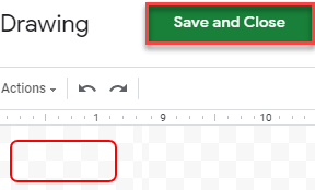
6. Now that the shape is created, and click Save and Close.

7. The shape is now inserted into the sheet, but not in the right place. Select the shape and position the cursor on it until the white hand appears. Now, drag and drop the shape to position it around cell B5 (Michael).

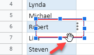
Finally, you have the red shape around the text.

Unfortunately, in Google Sheets, you can’t copy a drawing, so if you need several shapes, you’ll need to create them manually one by one.

Excel is one of my favorite spreadsheets due to its powerful formatting features. One can format content in the worksheet including cells, splitting it diagonally, and filling its two halves with different colors.

This article focuses on MS Excel for Windows Users. Demonstrating how o split a cell diagonally and apply to fill colors on its two halves. Follow the following procedure below.

The procedure for applying the format:

Step 1: Ensure that you have an updated and installed version of the MS Office suite.

Alternatively, you can have only the Excel application to be installed if possible.

Step 2:
Click the Windows button or optionally click Windows+ Q.

This will open the search option for most Windows OS versions. The search function is usually a faster way of searching an installed application in the Windows Operating system. It will optionally save you time.

Step 3: Ensure that the search functionality is resting on the apps option as shown below.

Step 4: Type in the word «excel» in the search Bar.

By typing the app name you initiate a Search operation for the MS Excel application for those who have already it installed.

As you type in more suggestions usually pop up.

Step 5: MS Excel will load its interface. Select your file of choice that you wish to open

Step 6: Now select the cell that you want to format.

The active cursor which is a bolded square border on a cell shows the currently highlighted cells.

Step 7: Right-click on the cell. You can do this using a mouse or laptop’s touchpad buttons.

A drop-down menu will be displayed as shown above.

Step 8: Select «Format Cells»

Format cells option is used to add appealing effects to the cell.

Step 9: A dialog box will be displayed. Click on the «Fill» tab.

Another dialog will appear. The dialog will have group boxes named colors, shading styles, variants, and a sample in the Right Bottom corner. The dialog also has «OK» and «CANCEL» buttons.

Step 10: Select the two colors that you want to fill in the cell. This is found at the «color 1» and «color 2 «drop-down selector.

Step 11: Select the «Diagonal up» or «diagonal down» radio button

Step 12: Click the «OK» button of the dialog.

Step 13: Also click ok for the other dialog named «format cells» to get the following result of the formatted cell.

Using shapes in cells

This is another method that is successful in splitting a cell into two. This method makes use of a shape that is inserted into the cell. The procedure for using this method is:

Step 1: Open Excel by either searching it or navigating to its location in the start menu.

Step 2: Click the Excel Icon.

Step 3: Wait for excel to load its interface. This should probably take a few seconds.

Step 4. Open the Excel file of your choice. Do this by navigating to the «File» then select «Open».

A list of files in your computer`s storage will be displayed. Choose the excel file that you wish to modify.

Step 4: Right-click on the cell that you want to apply the fill format.

Step 5: Select «Format cells» from the drop-down menu that appears.

Step 6: Choose a color from the Theme color Grid. In my case I choose yellow.

Step 7: Select the «OK» button.

The entire cell will now be formatted fully in the color you choose.

Step 8: Then, Click «insert tab» on the MS Excel ribbon. Then select Shapes.

Step 9: A dialog with all kinds of shapes will display. Double click on the Right-angled triangle.

You can optionally drag it into the cell you wish to format.

Step 10: Drag and resize the shape to split the yellow-filled cell diagonally.

Step 11: After the shape fits well right-click on it.

Step 12: Click on the «Format Shape» option.

Step 13: Select white as the fill color under the «Fill color» group box.

Step 14: Click on the close button of the dialog box.

With method two, your cell will now be split diagonally with a half white and half yellow section. Applying format onto a shape will create an impression on the cell. This is the basis of using method two to create a horizontal split in excel.

Using A Delimiter

Follow the below steps to split a cell diagonally from the middle and half-fill color in excel.

Step 1. Open the Excel spreadsheet you want to edit.

Step 2. Click and highlight the cells you want to split and half-fill color. Remember you can highlight cells with only one or more pieces of information. When dealing with wells with two or more pieces of information, you should separate them with a comma, dash, period, or space. For example, your column may read, “Nimrod, Europe.” In this case, you should highlight the desired cell and ensure a gray box appears.

Step 3. After this, click on the Data Tab at the top of your spreadsheet.

Step 4. After pressing this button, the data tab ribbon appears. Under the ribbon, select the Text to Columns option. A menu on Convert Text to Columns Wizard will appear.

Step 5. Now choose the “Delimited” button since you are using the Delimiter method.

Step 6. Still at the menu, click on the Next button at the bottom-right to choose your delimiters.

You should pick one or more delimiters to enable Excel to know where to split your cell. For instance, you can select the box next to the Comma delimiter since our data has a comma between Nimrod and Europe.

The Comma delimiter is common for data with names and addresses. Though, one may select the Space and Punctuation delimiters depending on your data, especially when extracting data from other sources and importing the data to a spreadsheet.

In other cases, some data may have multiple delimiters. For instance, in a row, you can have a comma followed by a space, or a semi-colon followed by a space. If this happens, you should pick all the delimiter boxes that apply to your data and tick the “Treat consecutive delimiters as one” box.

Step 7. Now press the Next button after you select all the delimiters that apply to your data.

Step 8. After this, choose the format option of how you want your data to appear on the column tab. You will find the below column formats on the menu. Select only one desired column format.

• General
• Text
• Date
• Do not import column(skip)

Step 9. Now click the Destination button to select where you want to place your new columns in Excel. For example, if the current information is in cell C3 and you want the cells next to it, type D3. Selecting “Destination” is an important step since failure to do it will have your split cells overwritten to your current cell.

Step 10. Press the Finish button that appears below on the menu to split your cells.

After splitting your cell, you now need to half-fill it with color diagonally. Here, you can follow these steps.

Step 1. Open the spreadsheet where you have the split cells.

Step 2. Select the split cells you want to diagonally half-fill with color and right-click.

Step 3. Now choose Format Cells in the drop-down menu that appears. Depending on your windows version, you may not see a drop-down menu. This is not a hindrance to diagonally half-fill your split cells with colors. Just select and right-click the split cells you want to diagonally half-fill with color and a drop-down menu will appear automatically. At the top of the menu, type Format Cells in the search bar and select the app that appears.

Step 4. Go to the Fill Tab and select Fill Effects.

Step 5. Now select the Two Colour check box and pick two colors you want to use in color 1 and color 2 respectively.

Step 6. Pick a shading style and choose the Diagonal Up variant.

Step 7. Select the diagonally colored window sample and click the OK button to apply the color. Now you have split and half-filled Excel cells diagonally with color in your workbook.

Using The Fixed Width Option

The Fixed Width option is used to manually split cells in excel. Below are steps to guide you through and half-fill a cell with colors.

Step 1. Open your Microsoft excel workbook that requires formatting.

Step 2. Highlight all the cells that need to be split. Unlike the Delimiter method, cells don’t need to have information separated by commas, punctuations, or spaces. Just select all the cells that you need to split.

Step 3. Go to the top of your Excel workbook and click on the Data Tab.

Step 4. Select the Texts to Columns button.

Step 5. After this, a Convert Text to Columns Wizard menu will appear. Select the Fixed Width option and click on the Next button at the bottom right.

Step 6. You should indicate at which point you would like to split your cell. Go to Data Preview and drag your line to the point you want a cell split. Remember, to remove an incorrect line split, you should double-click on the line.

Step 7. Press the Next button at the bottom right.

Step 8. After this, decide where to place the new spreadsheet cells. Under the Destination option, enter the row and the column where you need the split cells. Do not skip this step to avoid Excel overwriting the new cells to the current ones and making your data content difficult to read.

Step 9. Click on the Finish button.

Step 10. Select the range of split cells you want to diagonally fill half color.

Step 11. Press Ctrl + Shift + F command keys on your laptop keyboard.

Step 12. Next, go to the Fill Tab and choose Fill Effects at the bottom of the background colors.

Step 13. Check the Two-Color box and choose colors 1 and color 2 according to your preferences.

Step 14. Choose the Diagonal Down variant under the shading style and select the diagonally down-colored window.

Step 13. Lastly, click the OK button to diagonally apply the colors. You will have the cell split diagonally and half-filled with color.