Overview of formulas in Excel
Get started on how to create formulas and use built-in functions to perform calculations and solve problems.

Important: The calculated results of formulas and some Excel worksheet functions may differ slightly between a Windows PC using x86 or x86-64 architecture and a Windows RT PC using ARM architecture. Learn more about the differences.
Important: In this article we discuss XLOOKUP and VLOOKUP, which are similar. Try using the new XLOOKUP function, an improved version of VLOOKUP that works in any direction and returns exact matches by default, making it easier and more convenient to use than its predecessor.
Create a formula that refers to values in other cells
-
Select a cell.
-
Type the equal sign =.
Note: Formulas in Excel always begin with the equal sign.
-
Select a cell or type its address in the selected cell.

-
Enter an operator. For example, – for subtraction.
-
Select the next cell, or type its address in the selected cell.
-
Press Enter. The result of the calculation appears in the cell with the formula.


See a formula
-
When a formula is entered into a cell, it also appears in the Formula bar.
-
To see a formula, select a cell, and it will appear in the formula bar.


Enter a formula that contains a built-in function
-
Select an empty cell.
-
Type an equal sign = and then type a function. For example, =SUM for getting the total sales.
-
Type an opening parenthesis (.
-
Select the range of cells, and then type a closing parenthesis).
-
Press Enter to get the result.

Download our Formulas tutorial workbook
We’ve put together a Get started with Formulas workbook that you can download. If you’re new to Excel, or even if you have some experience with it, you can walk through Excel’s most common formulas in this tour. With real-world examples and helpful visuals, you’ll be able to Sum, Count, Average, and Vlookup like a pro.
Formulas in-depth
You can browse through the individual sections below to learn more about specific formula elements.
A formula can also contain any or all of the following: functions, references, operators, and constants.
Parts of a formula

1. Functions: The PI() function returns the value of pi: 3.142…
2. References: A2 returns the value in cell A2.
3. Constants: Numbers or text values entered directly into a formula, such as 2.
4. Operators: The ^ (caret) operator raises a number to a power, and the * (asterisk) operator multiplies numbers.
A constant is a value that is not calculated; it always stays the same. For example, the date 10/9/2008, the number 210, and the text «Quarterly Earnings» are all constants. An expression or a value resulting from an expression is not a constant. If you use constants in a formula instead of references to cells (for example, =30+70+110), the result changes only if you modify the formula. In general, it’s best to place constants in individual cells where they can be easily changed if needed, then reference those cells in formulas.
A reference identifies a cell or a range of cells on a worksheet, and tells Excel where to look for the values or data you want to use in a formula. You can use references to use data contained in different parts of a worksheet in one formula or use the value from one cell in several formulas. You can also refer to cells on other sheets in the same workbook, and to other workbooks. References to cells in other workbooks are called links or external references.
-
The A1 reference style
By default, Excel uses the A1 reference style, which refers to columns with letters (A through XFD, for a total of 16,384 columns) and refers to rows with numbers (1 through 1,048,576). These letters and numbers are called row and column headings. To refer to a cell, enter the column letter followed by the row number. For example, B2 refers to the cell at the intersection of column B and row 2.
To refer to
Use
The cell in column A and row 10
A10
The range of cells in column A and rows 10 through 20
A10:A20
The range of cells in row 15 and columns B through E
B15:E15
All cells in row 5
5:5
All cells in rows 5 through 10
5:10
All cells in column H
H:H
All cells in columns H through J
H:J
The range of cells in columns A through E and rows 10 through 20
A10:E20
-
Making a reference to a cell or a range of cells on another worksheet in the same workbook
In the following example, the AVERAGE function calculates the average value for the range B1:B10 on the worksheet named Marketing in the same workbook.
1. Refers to the worksheet named Marketing
2. Refers to the range of cells from B1 to B10
3. The exclamation point (!) Separates the worksheet reference from the cell range reference
Note: If the referenced worksheet has spaces or numbers in it, then you need to add apostrophes (‘) before and after the worksheet name, like =’123′!A1 or =’January Revenue’!A1.
-
The difference between absolute, relative and mixed references
-
Relative references A relative cell reference in a formula, such as A1, is based on the relative position of the cell that contains the formula and the cell the reference refers to. If the position of the cell that contains the formula changes, the reference is changed. If you copy or fill the formula across rows or down columns, the reference automatically adjusts. By default, new formulas use relative references. For example, if you copy or fill a relative reference in cell B2 to cell B3, it automatically adjusts from =A1 to =A2.
Copied formula with relative reference
-
Absolute references An absolute cell reference in a formula, such as $A$1, always refer to a cell in a specific location. If the position of the cell that contains the formula changes, the absolute reference remains the same. If you copy or fill the formula across rows or down columns, the absolute reference does not adjust. By default, new formulas use relative references, so you may need to switch them to absolute references. For example, if you copy or fill an absolute reference in cell B2 to cell B3, it stays the same in both cells: =$A$1.
Copied formula with absolute reference
-
Mixed references A mixed reference has either an absolute column and relative row, or absolute row and relative column. An absolute column reference takes the form $A1, $B1, and so on. An absolute row reference takes the form A$1, B$1, and so on. If the position of the cell that contains the formula changes, the relative reference is changed, and the absolute reference does not change. If you copy or fill the formula across rows or down columns, the relative reference automatically adjusts, and the absolute reference does not adjust. For example, if you copy or fill a mixed reference from cell A2 to B3, it adjusts from =A$1 to =B$1.
Copied formula with mixed reference
-
-
The 3-D reference style
Conveniently referencing multiple worksheets If you want to analyze data in the same cell or range of cells on multiple worksheets within a workbook, use a 3-D reference. A 3-D reference includes the cell or range reference, preceded by a range of worksheet names. Excel uses any worksheets stored between the starting and ending names of the reference. For example, =SUM(Sheet2:Sheet13!B5) adds all the values contained in cell B5 on all the worksheets between and including Sheet 2 and Sheet 13.
-
You can use 3-D references to refer to cells on other sheets, to define names, and to create formulas by using the following functions: SUM, AVERAGE, AVERAGEA, COUNT, COUNTA, MAX, MAXA, MIN, MINA, PRODUCT, STDEV.P, STDEV.S, STDEVA, STDEVPA, VAR.P, VAR.S, VARA, and VARPA.
-
3-D references cannot be used in array formulas.
-
3-D references cannot be used with the intersection operator (a single space) or in formulas that use implicit intersection.
What occurs when you move, copy, insert, or delete worksheets The following examples explain what happens when you move, copy, insert, or delete worksheets that are included in a 3-D reference. The examples use the formula =SUM(Sheet2:Sheet6!A2:A5) to add cells A2 through A5 on worksheets 2 through 6.
-
Insert or copy If you insert or copy sheets between Sheet2 and Sheet6 (the endpoints in this example), Excel includes all values in cells A2 through A5 from the added sheets in the calculations.
-
Delete If you delete sheets between Sheet2 and Sheet6, Excel removes their values from the calculation.
-
Move If you move sheets from between Sheet2 and Sheet6 to a location outside the referenced sheet range, Excel removes their values from the calculation.
-
Move an endpoint If you move Sheet2 or Sheet6 to another location in the same workbook, Excel adjusts the calculation to accommodate the new range of sheets between them.
-
Delete an endpoint If you delete Sheet2 or Sheet6, Excel adjusts the calculation to accommodate the range of sheets between them.
-
-
The R1C1 reference style
You can also use a reference style where both the rows and the columns on the worksheet are numbered. The R1C1 reference style is useful for computing row and column positions in macros. In the R1C1 style, Excel indicates the location of a cell with an «R» followed by a row number and a «C» followed by a column number.
Reference
Meaning
R[-2]C
A relative reference to the cell two rows up and in the same column
R[2]C[2]
A relative reference to the cell two rows down and two columns to the right
R2C2
An absolute reference to the cell in the second row and in the second column
R[-1]
A relative reference to the entire row above the active cell
R
An absolute reference to the current row
When you record a macro, Excel records some commands by using the R1C1 reference style. For example, if you record a command, such as clicking the AutoSum button to insert a formula that adds a range of cells, Excel records the formula by using R1C1 style, not A1 style, references.
You can turn the R1C1 reference style on or off by setting or clearing the R1C1 reference style check box under the Working with formulas section in the Formulas category of the Options dialog box. To display this dialog box, click the File tab.
Top of Page


Need more help?
You can always ask an expert in the Excel Tech Community or get support in the Answers community.
See Also
Switch between relative, absolute and mixed references for functions
Using calculation operators in Excel formulas
The order in which Excel performs operations in formulas
Using functions and nested functions in Excel formulas
Define and use names in formulas
Guidelines and examples of array formulas
Delete or remove a formula
How to avoid broken formulas
Find and correct errors in formulas
Excel keyboard shortcuts and function keys
Excel functions (by category)
Need more help?
Want more options?
Explore subscription benefits, browse training courses, learn how to secure your device, and more.
Communities help you ask and answer questions, give feedback, and hear from experts with rich knowledge.
How to Create a Formula in Excel: Beginner Tutorial (2023)
Excel is all about running calculations! And so creating and operating a formula in Excel is simple.
An Excel formula is a combination of operators and operands. For example, 2 + 2 = 4 is a formula where 2s are the operands, plus sign (+) is the operator, and 4 is the answer to the formula.
Only if you know the basics to write a formula in Excel – there’s a high chance you’d solve most of your Excel problems. This article explains the basics of creating Excel formulas.
So let’s dive right in.
As you scroll down, download our free sample workbook here to practice the examples used in the guide below. 😀
How to create formulas in Excel
Creating Excel formulas is easy as pie.
For example, what is 10 divided by 2? Can you calculate this in Excel?
1. Start by activating a cell.
2. Write an equal sign.

It is very important to start any formula with an equal sign. If you do not start with an equal sign, Excel wouldn’t recognize it as a formula but as a text string.
3. Input the simple mathematical operation of 10 divided by 2.
= 10 / 2

4. Hit enter, and you’re good to go!

You can create the same above formula with a slight variation.
For example, if you have the operands as cell values.

1. Write the formula using cell references as follows.
= A2 / B2

The above formula translates to ‘A2 divided by A3’.
Where A2 has the numeric value 10, and A3 has the numeric value 2.
2. The results remain the same as in the above example.

Creating a formula using cell references and values
The same formula can also be created using a combination of cell references and values.
Write the following formula using cell references and values.
= A2 / 2

The above formula translates to ‘A2 divided by 2’.
Where A2 has the numeric value 10, and 2 is a value.
1. The results look as follows.

Pro Tip!
Using cell references is better than using absolute values. This is because if sometime later you change the cell value – the formula would automatically update.
How to add, subtract, multiply, and divide?
There are four basic mathematical operations – add, subtract, multiply, and divide.
Let’s now see how to perform each of these operations in Excel.
How to make a SUM formula (addition)
Adding things up in Excel can take different forms.
Excel has an in-built function for performing addition i.e. the SUM function. Here’s how you can bring it to action.
1. Write the SUM function beginning with an equal sign as follows.
= SUM (5, 5)
Every argument of the SUM function separated by a comma represents the value to be added.
Excel adds 5 into 5 to give the results below.

Easy enough? You can use the SUM function for cell references too. 🤩
2. Write the SUM function as follows.
= SUM (A2, A3)
Pro Tip!
To insert SUM from the Insert Function button, take this route.
Go to Formulas tab > Function Library > Insert function button > Type the function name.
In the Insert Function dialog box, type SUM and hit search. Select the desired function and hit ‘Okay’ to insert the same.
Excel adds the cell values of Cell A2 and Cell A3.

What makes the SUM function a big plus is its ability to add up a range of cells.
For example, see the data below.

3. To add this up in Excel using the SUM function, write the SUM function as below.
= SUM (A2:A10)

Must notice how we have defined the cell range from Cell A2 to Cell A10 as A2:A10.
4. Excel sums up all cell values in cells from A2 to A10.

You can make this function work even more interestingly by adding up multiple ranges.
5. Write the SUM function with multiple ranges as follows.
= SUM (A2:A5, B2:B8, C1:C10)


How to subtract in Excel
Subtracting in Excel is all about creating a formula with the minus sign operator (-).
For example:
1. To subtract 5 from 10, begin with an equal sign and write the following formula.
= 10 – 5
A simple subtraction formula with a minus sign operator!
Press enter and here you go.

2. Try doing the same with cell references as below.
= A2 – A3
This formula translates to A2 less A3. Where A2 has the numeric value 10, and A3 has the numeric value 5.

3. Alternatively, you can use the SUM function to perform subtraction. However, to do this you need to add a minus sign to the value to be subtracted.
= SUM (A2, -A3)
Here are the results.

How to multiply in Excel
After we have learned how to add and subtract in Excel, it’s time we learn multiplication in Excel.
First thing first, the operator for multiplication in Excel is an asterisk (*).
Now, do you remember what is 9 times 8? No?
1. Write a multiplication formula in Excel.
= 9 * 8


2. Try doing the same using cell references as below.
= A2 * A3

The formula above translates to A2 multiplied by A3.
Excel also offers an in-built function for multiplication in Excel. The PRODUCT Function!
3. Write the PRODUCT function as follows.
= PRODUCT (9, 

We have added both the values to be multiplied as the arguments to the PRODUCT function.
Here are the results.

The PRODUCT function can also find the product of multiple values (or a range of cells) at once.
For example, see the data below.

4. To multiply all these values, write the PRODUCT function as follows:
= PRODUCT (A2:A10)

Excel multiplies all the values in the specified range.

How to divide in Excel
Here comes the last operation of this guide – division. 🤞
Creating a division formula in Excel is also very straightforward.
What is the operator for division? A forward slash (/).
Also, the dividend (or the numerator) comes before the slash. And the divisor (or the denominator) comes after the slash.
1. Write a division formula as below.
= 30 / 10

Excel divides both operands to give the results as follows.

2. The same can be done using cell references.
= A2 / A3
Pro Tip!
While performing the division function in Excel, you might see the #DIV/0! Error. This error is given back by Excel when you attempt to divide the number of zero.
Basic Rule of Grade 6! No number is divisible by zero. Excel remembers that, if not us. 😆
Order of operations
Here’s an equation for you to solve.
= 2+ 4 * 6 / 3 – 2
What a mess! Which operation do you perform first?
To solve this mystery, there is an order for performing mathematical operations – PEMDAS
P = Parenthesis
E = Exponents
MD = Multiplication & Division (left to right)
AS = Addition & Subtraction
Solve the above equation in the same order, and you’d reach the answer 8.
Let Excel do the same to see the results.

Excel performs division first (6 / 3 = 2), multiplication second (4 * 2 = 8), addition third (2 + 8 = 10), and subtraction last (10 – 2 = 8), resulting in 8.
Now, let’s enclose a part of this formula in parentheses to see how the results change.
= 2+ 4 * 6 / (3 – 2)

What causes the results to change with only parenthesis added?
Excel now first performs the operation enclosed in parenthesis i.e. (3-2).
Next, multiplication is performed, then division and addition last. This causes the answer to change.
Pro Tip!
Try doing some mental maths to double-check if Excel has rightly calculated 26.
Parenthesis first = 2+ 4*6/(3 – 2)
Multiplication Second= 2+4*6/1
Division Third = 2 + 24/1
Addition Last = 2 + 24
Here’s the answer = 26
How to create formulas with references
Creating Excel formulas with references is super simple. All you need to do is replace the values in a simple formula with cell references (cells that contain those values).
For example, let’s create a multiplication formula in Excel.

Great! What if you had 2 & 4 as numerical values in cells?

Create the same formula using cell references.

You can do the same for all operators! It is this simple.
Also, what happens when a cell value changes? Until the cell reference is in place, the formula would automatically update for the cell value change.

Must note how the cell reference in the formula remains unchanged. The answer however changes as the cell value for A3 has changed.ltiple criteria lookup💡
Formulas or functions?
What is an Excel formula, and what is an Excel function? And how are these two different?
There are two ways to add 2 and 2 in Excel.
- = 2 + 2
- SUM (2,2)
The answer to them both would be the same. However, the first one is a formula created in Excel. Whereas the second one is an in-built function of Excel – the SUM function.
Functions are more like predefined formulas in Excel.
Although the function library of Microsoft Excel is huge enough for you to explore, there is a limit to it. And you may not find everything you need there.
So, you might still need to write your own formulas to perform calculations in Excel. 😉
Pro Tip!
Sometimes, you might even nest a function into a formula.
For example, what is 2 + 2 – 3?
You may write it as = (SUM (2,2)) – 3
SUM (2,2) is a function, and deducting 3 from it makes it a self-created formula.
That’s it – Now what?
Until now, we’ve created formulas using different operators, values, and cell references. And learned how to use the SUM function for addition and subtraction.
Not only that but we’ve also studied the order of operations in Excel. The above article is a whole pack of information, isn’t it?
Creating your own formulas in Excel is the first step to manipulating numbers in Excel. However, this is something very basic, and Excel has tons more to offer.
Some very important Excel functions that one must hone include the VLOOKUP, SUMIF, and IF functions.
Haven’t mastered them yet? Click here to register for my 30-minute free email course that helps you learn these and much more.
Kasper Langmann2023-02-23T14:38:38+00:00
Page load link
Содержание
- Создание простейших формул в Excel
- Примеры вычислений в Excel
- Использование Excel как калькулятор
- Основные операторы Excel
- Вопросы и ответы

Одной из основных возможностей Microsoft Excel является возможность работы с формулами. Это значительно упрощает и ускоряет процедуру подсчета общих итогов и отображения искомых данных. Давайте разберемся, как создать формулы и как работать с ними в программе.
Самыми простыми формулами в Экселе являются выражения арифметических действий между данными, расположенными в ячейках. Чтобы создать подобную формулу, прежде всего пишем знак равенства в ту ячейку, в которую предполагается выводить полученный результат от арифметического действия. Либо можете выделить ячейку, но вставить знак равенства в строку формул. Эти манипуляции равнозначны и автоматически дублируются.

Затем выделите определенную ячейку, заполненную данными, и поставьте нужный арифметический знак («+», «-», «*»,«/» и т.д.). Такие знаки называются операторами формул. Теперь выделите следующую ячейку и повторяйте действия поочередно до тех пор, пока все ячейки, которые требуются, не будут задействованы. После того, как выражение будет введено полностью, нажмите Enter на клавиатуре для отображения подсчетов.
Примеры вычислений в Excel
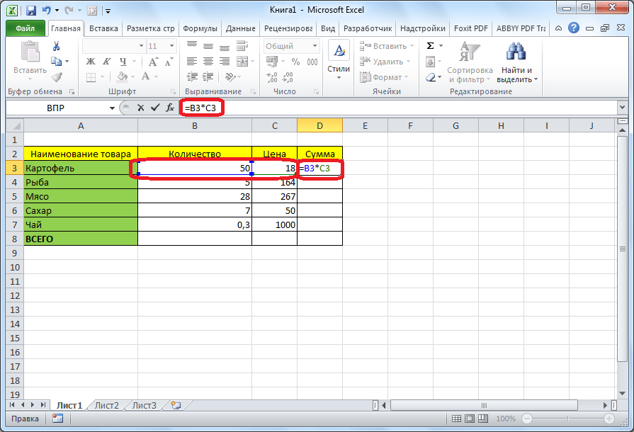
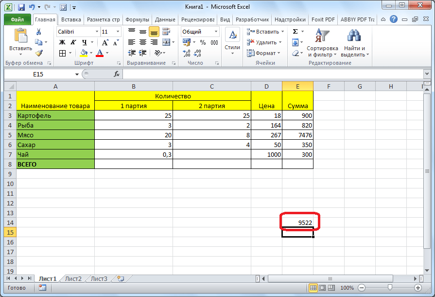
Допустим, у нас есть таблица, в которой указано количество товара, и цена его единицы. Нам нужно узнать общую сумму стоимости каждого наименования товара. Это можно сделать путем умножения количества на цену товара.
- Выбираем ячейку, где должна будет отображаться сумма, и ставим там =. Далее выделяем ячейку с количеством товара — ссылка на нее сразу же появляется после знака равенства. После координат ячейки нужно вставить арифметический знак. В нашем случае это будет знак умножения — *. Теперь кликаем по ячейке, где размещаются данные с ценой единицы товара. Арифметическая формула готова.
- Для просмотра ее результата нажмите клавишу Enter.
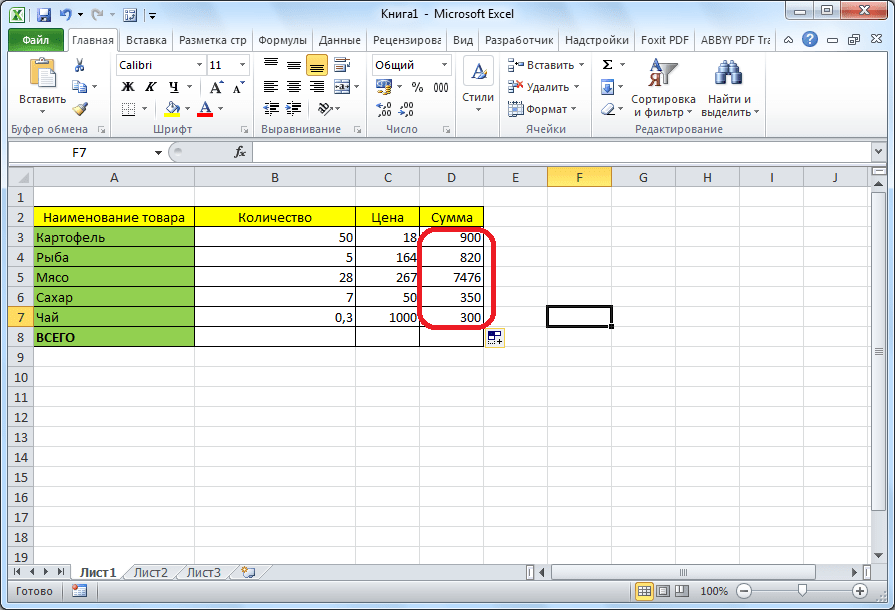
- Чтобы не вводить эту формулу каждый раз для вычисления общей стоимости каждого наименования товара, наведите курсор на правый нижний угол ячейки с результатом и потяните вниз на всю область строк, в которых расположено наименование товара.
- Формула скопировалась и общая стоимость автоматически рассчиталась для каждого вида товара,согласно данным о его количестве и цене.


Аналогичным образом можно рассчитывать формулы в несколько действий и с разными арифметическими знаками. Фактически формулы Excel составляются по тем же принципам, по которым выполняются обычные арифметические примеры в математике. При этом используется практически идентичный синтаксис.
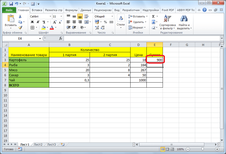
Усложним задачу, разделив количество товара в таблице на две партии. Теперь, чтобы узнать общую стоимость, следует сперва сложить количество обеих партий товара и полученный результат умножить на цену. В арифметике подобные расчеты выполнятся с использованием скобок, иначе первым действием будет выполнено умножение, что приведет к неправильному подсчету. Воспользуемся ими и для решения поставленной задачи в Excel.
- Итак, пишем = в первой ячейке столбца «Сумма». Затем открываем скобку, кликаем по первой ячейке в столбце «1 партия», ставим +, щелкаем по первой ячейке в столбце «2 партия». Далее закрываем скобку и ставим *. Кликаем по первой ячейке в столбце «Цена» — так мы получили формулу.
- Нажимаем Enter, чтобы узнать результат.
- Так же, как и в прошлый раз, с применением способа перетягивания копируем данную формулу и для других строк таблицы.
- Нужно заметить, что не обязательно все эти формулы должны располагаться в соседних ячейках или в границах одной таблицы. Они могут находиться в другой таблице или даже на другом листе документа. Программа все равно корректно осуществляет подсчет.


Использование Excel как калькулятор
Хотя основной задачей программы является вычисление в таблицах, ее можно использовать и как простой калькулятор. Вводим знак равенства и вводим нужные цифры и операторы в любой ячейке листа или в строке формул.


Для получения результата жмем Enter.
Основные операторы Excel
К основным операторам вычислений, которые применяются в Microsoft Excel, относятся следующие:
| Оператор | Описание | Действие |
|---|---|---|
| = | Знак равенства | Равно |
| + | Плюс | Сложение |
| — | Минус | Вычитание |
| * | Звездочка | Умножение |
| / | Наклонная черта | Деление |
| ^ | Циркумфлекс | Возведение в степень |
Microsoft Excel предоставляет полный инструментарий пользователю для выполнения различных арифметических действий. Они могут выполняться как при составлении таблиц, так и отдельно для вычисления результата определенных арифметических операций.
Еще статьи по данной теме:
Помогла ли Вам статья?
Spreadsheets aren’t merely for arranging data into rows and columns. Most of the time, you use them for data analysis as well.
Microsoft Excel is one of the most widely used spreadsheet applications, especially in finance and accounting. This is partly because of its easy UI and unmatched depth of functions.
In this article, you will learn:
- What Excel formulas are
- How to write a formula in Excel
- What Excel functions are
- How to work with an Excel function
- Lastly, we’ll take a look at dynamic Excel functions.
What do I need to install on my computer to follow this article?
To follow along, you will need to have Microsoft Excel installed on your computer. We’ll use a Windows computer for this article.
How can I install Microsoft Excel on my computer?
Follow these steps to install Microsoft Excel on your Windows computer:
- Sign in to www.office.com if you’re not already signed in.
- Sign in with the account associated with your Microsoft 365 subscription. You can also try out Office for free as well.
- Once signed in, select “Install Office” from the Office home page. This will automatically download Microsoft Office onto your Windows computer.
- Run the installer to set up Microsoft Office and select «Close» once you’re done.
- Once done, select the “Start” button (located at the lower-left corner of your screen) and type “Microsoft Excel.”
- Click on Microsoft Excel to open it.
- Accept the license agreement, and let’s get started.
What are Excel Formulas?
An Excel formula is an expression that carries out an operation based on the value of a cell or range of cells. You can use an Excel formula to:
- Perform simple mathematical operations such as addition or subtraction.
- Perform a simple operation like joining categorical data.
It’s important to understand two things: Excel formulas always begin with the equals «=» sign and they can return an error if not properly executed.
What Operators Are Used in Excel Formulas?
There are four different types of operators in Excel—arithmetic, comparison, text concatenation, and reference. But for most formulas, you’ll typically use these three:
Arithmetic operators
|
+ |
Addition |
|
— |
Subtraction |
|
/ |
Division |
|
* |
Multiplication |
|
^ |
Exponentiation |
Comparison operators
|
= |
Equal to |
|
> |
Greater than |
|
< |
Less than |
|
>= |
Greater than or equal to |
|
<= |
Less than or equal to |
|
<> |
Not equal to |
Text concatenation
Here you have just the ampersand “&” sign for joining text.
How Can I Create an Excel Formula?
Let’s take a simple scenario using one of the arithmetic operators.
In math, to add up two numbers, let’s say 20 and 30, you will calculate this by writing: 20 + 30 =
And this will give you 50.
In Excel, here is how it goes:
- First, open a blank Excel worksheet.
- In cell A1, type 20.
- In cell A2, type 30.
- To add it up, type in = 20 + 30 in cell A3.

5. Then, press ENTER on your keyboard. Excel will instantly calculate this and return 50.

I mentioned earlier that every formula begins with the equal «=» sign. That’s what I meant. To write a formula, you type the equal to sign followed by the numeric values. This also applies to cases of subtraction, division, multiplication, and exponentiation.
Let’s take another simple scenario using one of the comparison operators. Assume we want to find out if 30 is greater than 40.
In Excel, here is how we would do it:
- Type in =30>40
- Press ENTER.

3. This will return a FALSE because 30 isn’t greater than 40. Excel uses TRUE and FALSE for logical statements, the same way we human says yes and no.

Lastly, let’s take another simple scenario using the text concatenation operator – the ampersand “&” sign. This works with your string data types and you use it to join text.
Assume we have «Welcome», «To», and «FreeCodeCamp» all in different cells—A1, A2, and A3—of your worksheet. We would type =A1&” “&A2&” “&A3 to join them.
The space in quotes “ “ represents that we want a space between our words.

Another tip: the formula bar shows the formula used to generate a value.
What Are Excel Functions?
Excel functions are predefined inbuilt formulas that perform mathematical, statistical, and logical calculations and operations using your values and arguments.
For Excel functions, you should know that:
- They’re formulas, so yeah, they start with the equal «=» sign as well.
- The order is very important.
There are over 500 functions available. You can find all available Excel functions on the Formulas tab on the Ribbon.

But why use a function when you can just write a formula?
Here are some benefits of Excel functions.
- To improve productivity and effectiveness.
- To simplify complex calculations.
- To automate your work.
- To quickly visualize data.
What Makes Up Excel Functions?
Unlike formulas, Excel functions are made up of a structure with arguments you need to pass.
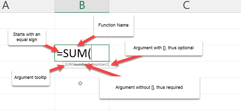
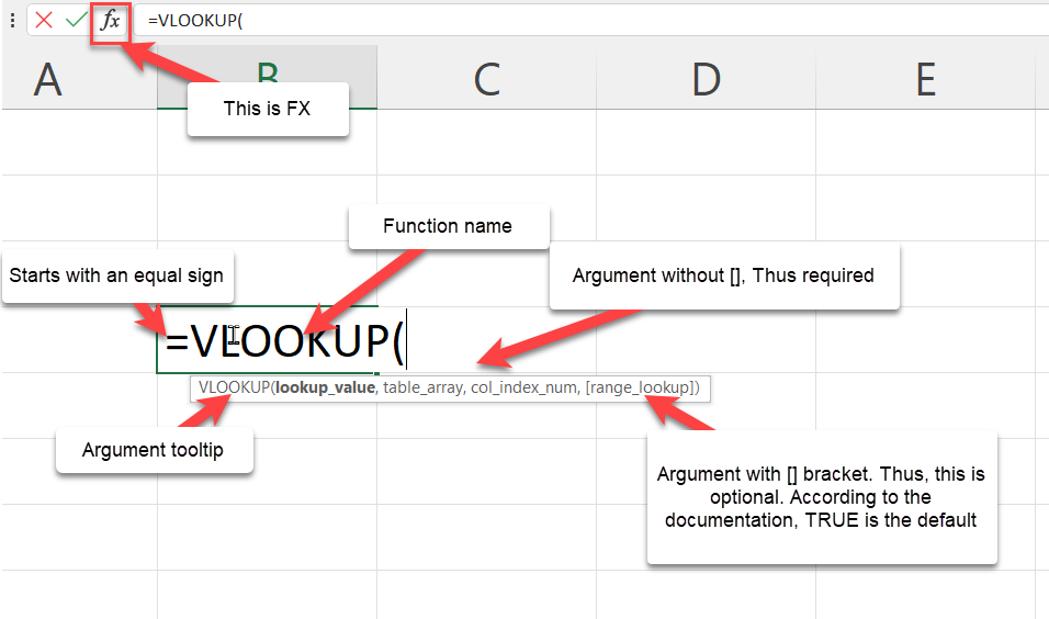
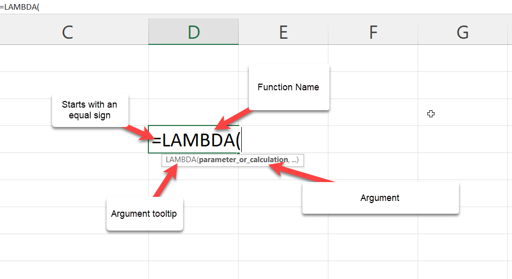
Every function:
- Starts with the equals «=» sign
- Has a name. Some examples are VLOOKUP, SUM, UNIQUE, and XLOOKUP.
- Requires arguments which are separated by commas. You should know that semicolons are used as separators in countries like Spain, France, Italy, Netherlands, and Germany. You can, however, change this via the Excel setting.
- Argument with the square brackets [] are optional
- Has an opening and closing parenthesis.
- Has an argument tooltip which shows you what you should pass.
There are some exceptions. For example,
- The DATEDIF doesn’t show in Excel because it is not a standard function and gives incorrect results in a few circumstances. However, here is the syntax:
DATEDIF(birthdate, TODAY(), "y")
- Functions like PI(), RAND(), NOW(), TODAY() require no argument.
Let’s look at a few functions:
How to Use the SUM() Function in Excel
According to the documentation, the SUM function adds values. Here is the syntax:
Let’s assume that we have a line of numbers from 1 to 10 and we want to add it up. To achieve this, we will just type =SUM(A1:A10). The A1:A10 simply returns an array of number that are situated on cell A1 to A10 which are A1, A2, and A3 up through A10.

Since the second argument is optional, that means a sum(A10) will return a value. In our case, it will return just 10 since A10 has the value 10 in it. Give it a try.
If you were writing this using the addition operator, you would have written:
=1 + 2 + 3 + 4 + 5 + 6 + 7 + 8 + 9 + 10
or
=A1 + A2 + A3 + A4 + A5 + A6 + A7 + A8 + A9 + A10
This doesn’t look very productive or efficient.
How to Use the TODAY() Function in Excel
According to the documentation, the TODAY function displays the current date on your worksheet. It also requires no argument. Here is the syntax:

Excel displays the current date automatically according to your computer’s date and time setting. The same goes for the NOW() function, which displays the current date and time.
How to Use the CONCATENATE() Function in Excel
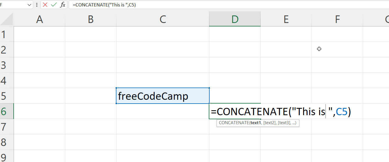
Let’s look at a text function. You use CONCATENATE to join two or more text strings into one string together.
Here is the syntax:

Let’s assume we want to join “This is” with “freeCodeCamp” – but in your cell, you have just «freeCodeCamp.»
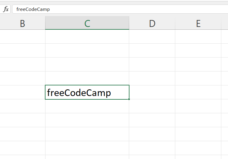
If you’re going to write a string inside a formula, you must write it inside quotes like this “ “.
Why?
This way, Excel wouldnt think you’re trying to write another function.
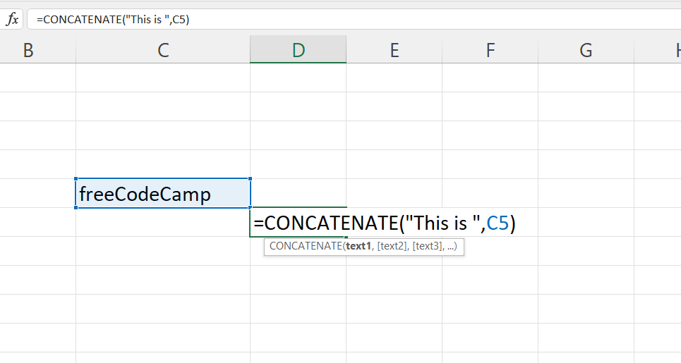
This will return the phrase “This is freeCodeCamp”
How to Use the VLOOKUP() Function in Excel
This is one of Excel’s most interesting and commonly used formulas or functions. You use it to find a value in a table or range by row.
Here is a scenario:
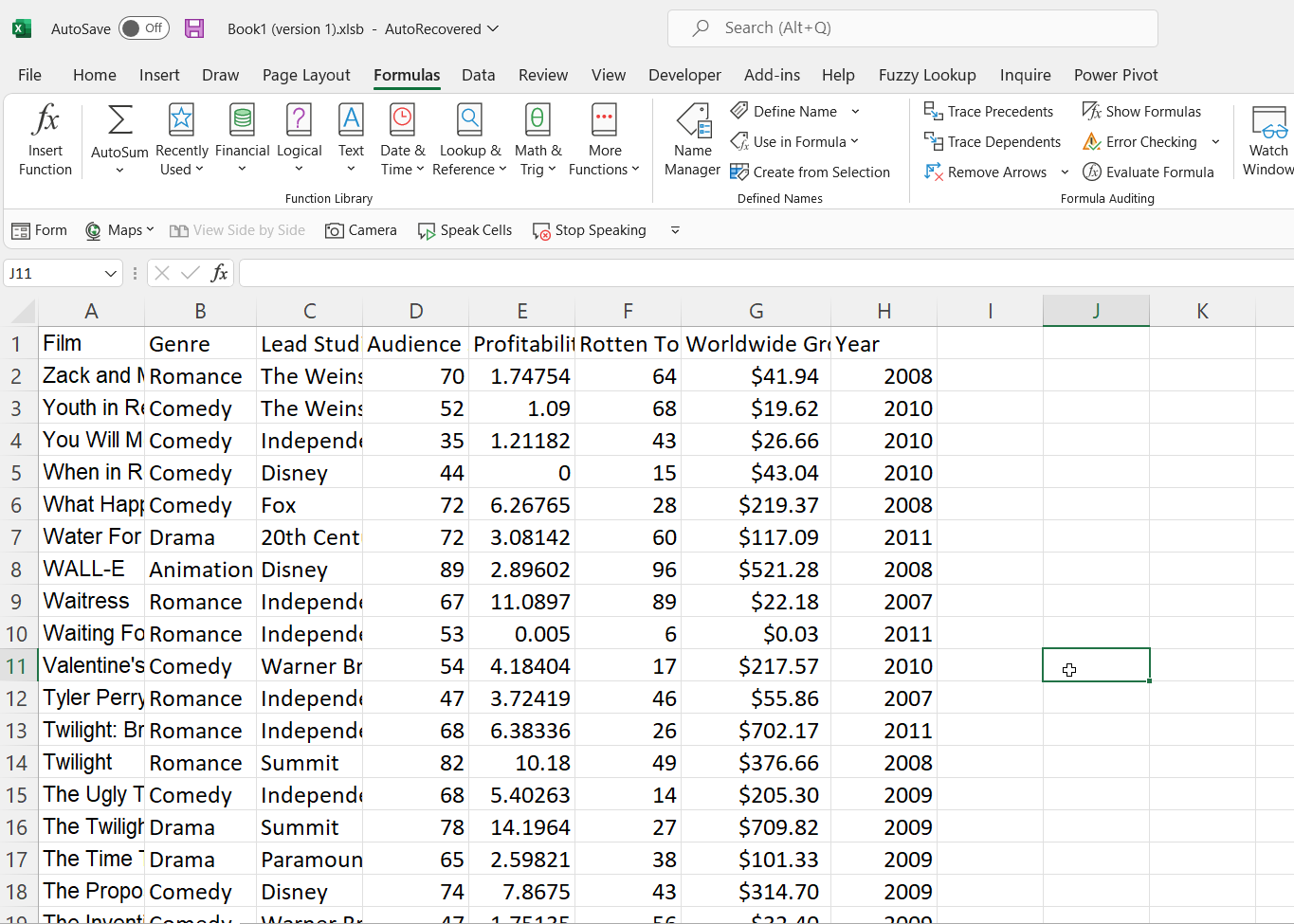
We have a simple table that shows various films along with their genre, lead studio, audience score %, profitability, rotten tomatoes %, worldwide gross and year. I would use just the first 10 rows of the sample data from this GitHub Gist.

I want that, whenever I type in a movie in the yellow cell, the year should get displayed in the green cell. Let’s use VLOOKUP to find it.
This is the VLOOKUP syntax:
Besides writing your formulas in the cell, you can also write them using the Excel Insert Function (fx) button, which is close to the formula bar.
Let’s try this.
- Write
=Vlookup(on the green cell. - Click on fx. A dialogue box will pop up showing all the arguments this formula needs.
- Input the value for each argument.
- Lookup_value (required argument): This is what you want to find. In our case, that is the movie “Youth in Revolt” which is in cell B1.
- Table_array (required argument): This is just asking you for the table that contains the data. You give it the entire table, which in our case is A4:H13
- Col_index_num (required argument): This is asking you for the column number of the table you gave. In our case, we want the year. This is in column 8.
- Range_lookup (optional argument): Lastly, we pick if we want an approximate match (TRUE) or an exact match (FALSE).
— TRUE means approximate match, so it returns the closest or an estimate.
— FALSE means exact match, so it returns an error if it’s not found.
8. We would go for the FALSE because we want the exact match.

9. Click on «OK.» Excel will return 2010.
However, you can write this in the cell by typing in =VLOOKUP(B1,A4:H13,8,FALSE) in your cell.

Tips and Rules When Writing Excel Functions
When writing our function, Excel provides some formula tips.
- The Argument tooltip doesn’t leave until you close the last parenthesis.
- The formula bar shows your formula.
- The argument you are currently writing is always dark. Take a look at the lookup_value in the image below.
- The square brackets [] tell you it is optional.
- Lastly, the colour code – our B1 is in blue, and cell B1 is in blue to guide us on what cell or table was picked. The same thing will happen to A4:H13 when we pick it as our table_array argument.

How to Work with Nested Functions in Excel
A nested function is when you write a function within another function. For example, finding the average of the sum of values.
The first tip when writing a nested function will be to treat every function individually. So address the first function before addressing the second. A pro tip would be to look at the argument tooltip when writing it.
Let’s take a simple scenario.
We have two arrays of numbers. Each has the scores of students in the class. I want to add the two arrays before I get the average.
Let’s get started.
- Type in your = followed by the average.
- The number one will be the sum of the scores from class one.
- The number two will be the sum of the scores from class two.
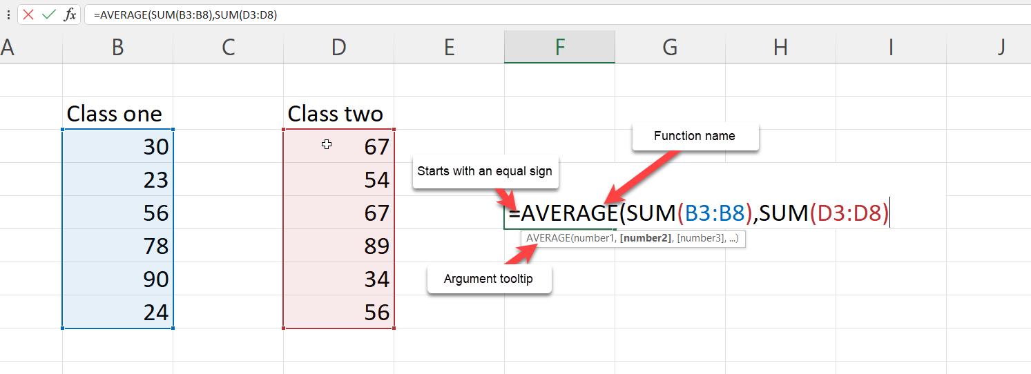

Finally, don’t forget the closing parenthesis.
Thus, the formula will be =AVERAGE(SUM(B3:B8),SUM(D3:D8)).
How to Work with Dynamic Array Functions in Excel
Dynamic array functions are formulas associated with spill array behaviour.
Before now, you wrote a function and it returned just a single input. We call these kinds of functions legacy array formulas.
Dynamic array functions, on the other hand, will return values that will enter the neighbouring cells. A few examples of dynamic array functions are:
- UNIQUE
- TEXTSPLIT
- FILTER
- SEQUENCE
- SORT
- SORTBY
- RANDARRAY
Let’s look at the UNIQUE formula.
How to Use the UNIQUE() Formula in Excel
The unique formula works by returning the unique value from an array or list. Let’s use the movie sample data from this GitHub Gist. This table contains 77 rows of film excluding the heading.

Let’s try to get the unique years from our dataset – that is, years without duplicates.
To do this:
- Type
=UNIQUE( - Select the entire array of values from the year column: =UNIQUE(H2:H78)

3. Close the parenthesis and press Enter.
Though the formula was written in a single cell, the returned value got spilled into the cells below it. That’s the spilled array behaviour.

How to Create Your Own Functions in Excel
Microsoft Excel released a bunch of new functions to make user more productive. One of these function was the LAMBDA function.
The LAMBDA function lets you create custom functions without macros, VBA or JavaScript, and reuse them throughout a workbook.
The best part? you can name it.
How to Use the LAMBDA() Function in Excel
This LAMBDA function will increase productivity by eliminating the need to copy and paste this formula, which can be error-prone.
Here is the LAMBDA syntax:
Lets start with a simple use case using the movie sample data from this GitHub Gist.
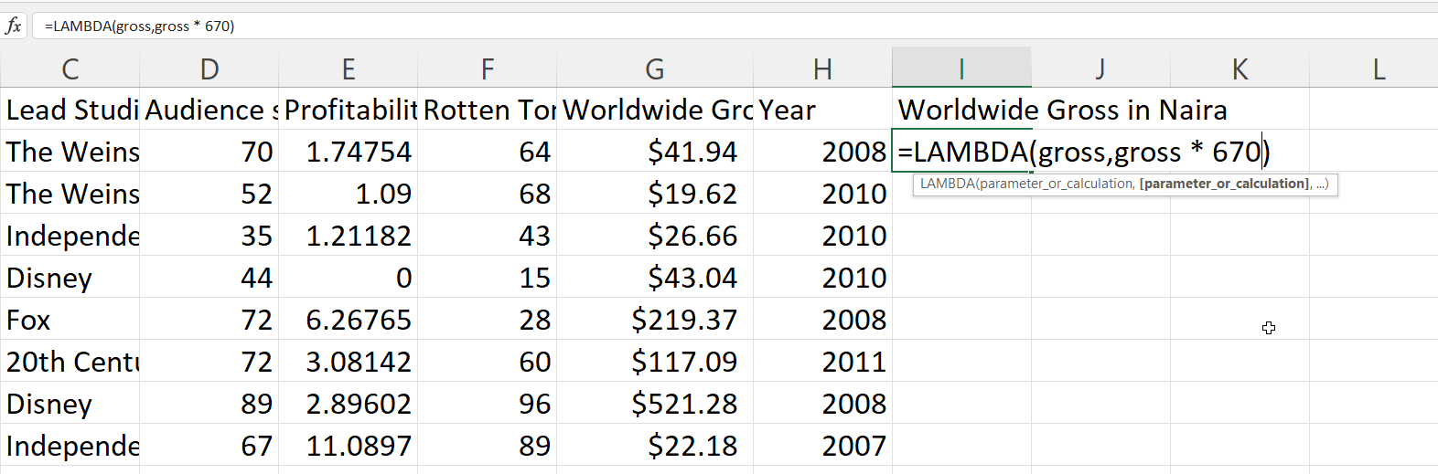
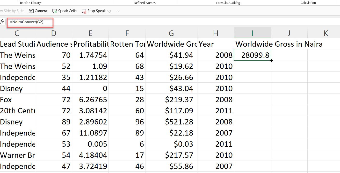
We had a column called «Worldwide Gross», lets try to find the Naira value.
- Create a new column and call it «Worldwide Gross in Naira».
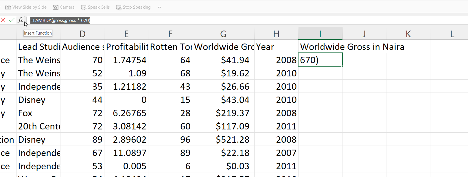
- Right below our column name, Cell I2, type
=lAMBDA( - LAMBDA requires a parameter and/or a calculation.
The parameter means the value you want to pass, in our use case we want to change the gross value. Lets call it gross.
The calculation means the formula or function you want to execute. For us, that will be to multiply it with te exchange rate. At the moment, that’s 670. so lets write gross * 670.
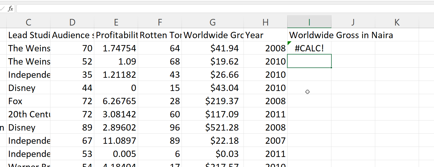
4. Press Enter. This will return an error because, gross doesnt exist and you need to let excel know of these names.
5. To make use of the newly created function, you need to copy the syntax written.
6. Go to the formula ribbon and open the name manager.
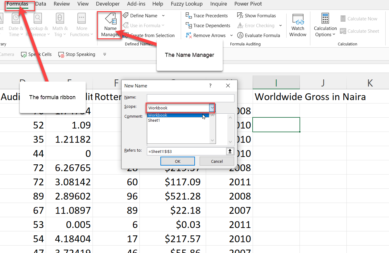
7. Define the name manger parameters:
- The name is simply what you want to call this function. I am going with NairaConvert.
- The scope should be workbook because you want to use this function in the workbook.
- The comments explains what your function does. It is acts as a documentation.
- In the refer to, you should paste the copied function syntax.
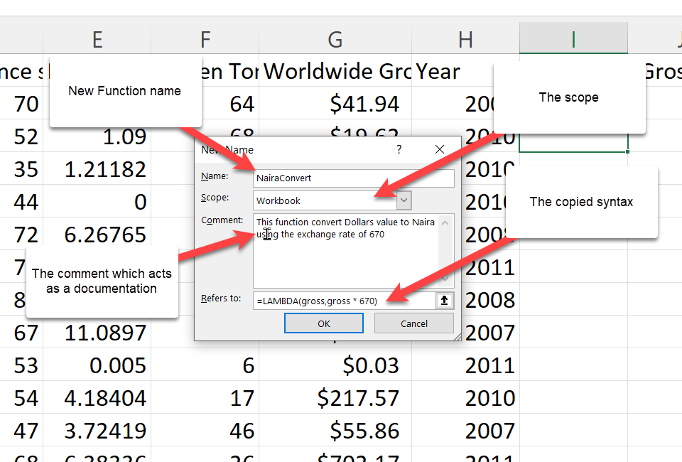
8. Press Ok.
9. To use this new function, you call it with the name you defined it as—NairaConvert—and give it the gross which is our worldwise gross on G2.
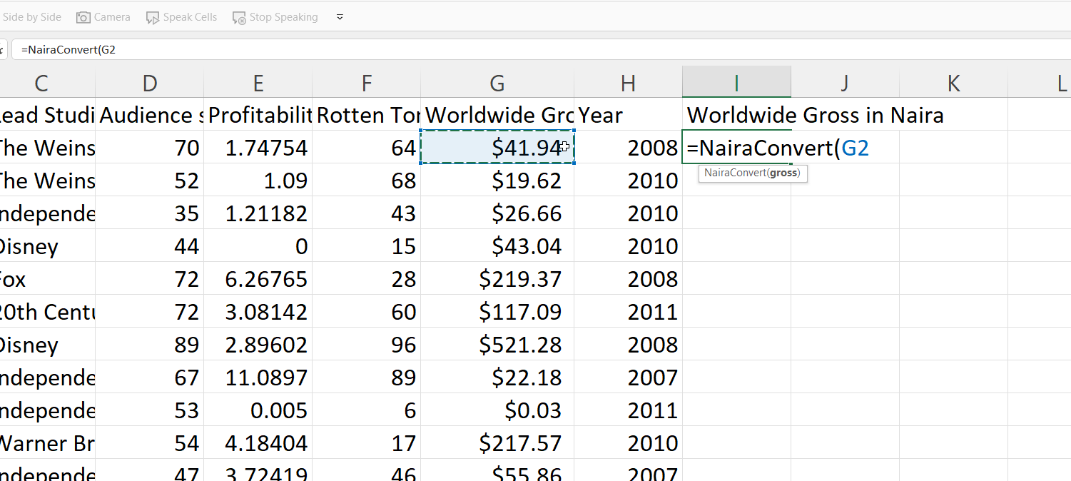
10. Close the parenthesis and press Ok
Where Can I Learn More about Excel?
There are a ton of resources for learning Microsoft Excel nowadays. So many that it is hard to figure out which ones are up-to-date and helpful.
The best thing you can do is find a helpful tutorial and follow it to completion, instead of attempting to take several at once. I would advise you to start with freeCodeCamp’s Microsoft Excel Tutorial for Beginners — Full Course, which is available on YouTube.
You should also join communities like the Microsoft Excel and Data Analysis Learning Community. However, if you’re looking for a compilation of resources, check out freeCodeCamp’s publication Excel tags.
If you enjoyed reading this article and/or have any questions and want to connect, you can find me on LinkedIn or Twitter.
Learn to code for free. freeCodeCamp’s open source curriculum has helped more than 40,000 people get jobs as developers. Get started
Excel formulas allow you to identify relationships between values in your spreadsheet’s cells, perform mathematical calculations with those values, and return the resulting value in the cell of your choice. Sum, subtraction, percentage, division, average, and even dates/times are among the formulas that can be performed automatically. For example, =A1+A2+A3+A4+A5, which finds the sum of the range of values from cell A1 to cell A5.
Excel Functions: A formula is a mathematical expression that computes the value of a cell. Functions are predefined formulas that are already in Excel. Functions carry out specific calculations in a specific order based on the values specified as arguments or parameters. For example, =SUM (A1:A10). This function adds up all the values in cells A1 through A10.
How to Insert Formulas in Excel?
This horizontal menu, shown below, in more recent versions of Excel allows you to find and insert Excel formulas into specific cells of your spreadsheet. On the Formulas tab, you can find all available Excel functions in the Function Library:
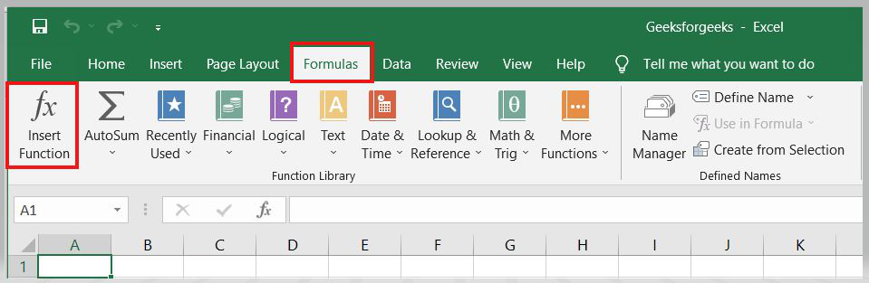
The more you use Excel formulas, the easier it will be to remember and perform them manually. Excel has over 400 functions, and the number is increasing from version to version. The formulas can be inserted into Excel using the following method:
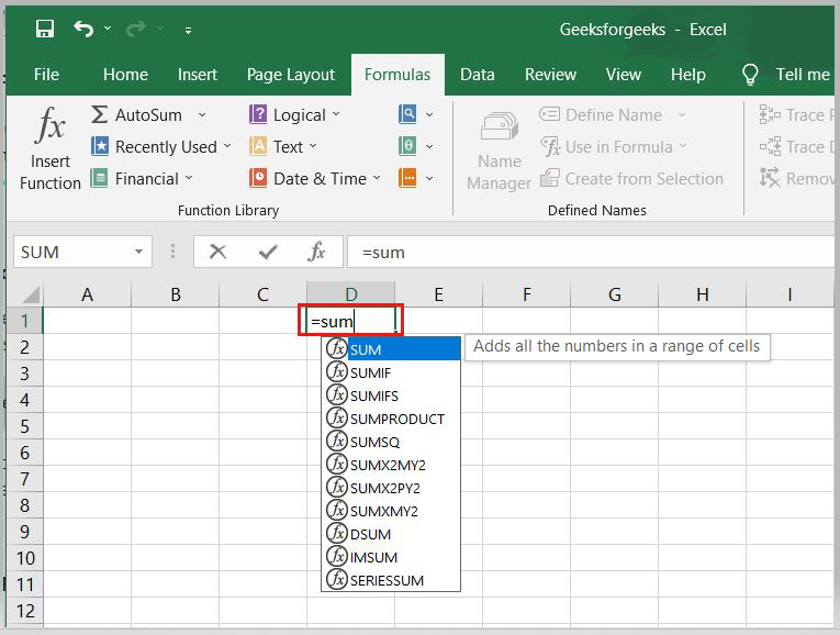
1. Simple insertion of the formula(Typing a formula in the cell):
Typing a formula into a cell or the formula bar is the simplest way to insert basic Excel formulas. Typically, the process begins with typing an equal sign followed by the name of an Excel function. Excel is quite intelligent in that it displays a pop-up function hint when you begin typing the name of the function.
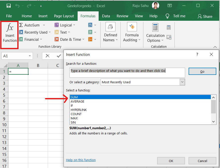
2. Using the Insert Function option on the Formulas Tab:
If you want complete control over your function insertion, use the Excel Insert Function dialogue box. To do so, go to the Formulas tab and select the first menu, Insert Function. All the functions will be available in the dialogue box.
3. Choosing a Formula from One of the Formula Groups in the Formula Tab:
This option is for those who want to quickly dive into their favorite functions. Navigate to the Formulas tab and select your preferred group to access this menu. Click to reveal a sub-menu containing a list of functions. You can then choose your preference. If your preferred group isn’t on the tab, click the More Functions option — it’s most likely hidden there.
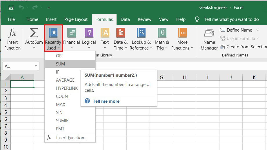
4. Use Recently Used Tabs for Quick Insertion:
If retyping your most recent formula becomes tedious, use the Recently Used menu. It’s on the Formulas tab, the third menu option after AutoSum.
Basic Excel Formulas and Functions:
1. SUM:
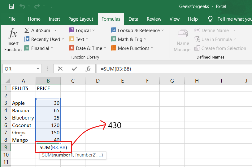
The SUM formula in Excel is one of the most fundamental formulas you can use in a spreadsheet, allowing you to calculate the sum (or total) of two or more values. To use the SUM formula, enter the values you want to add together in the following format: =SUM(value 1, value 2,…..).
Example: In the below example to calculate the sum of price of all the fruits, in B9 cell type =SUM(B3:B8). this will calculate the sum of B3, B4, B5, B6, B7, B8 Press “Enter,” and the cell will produce the sum: 430.
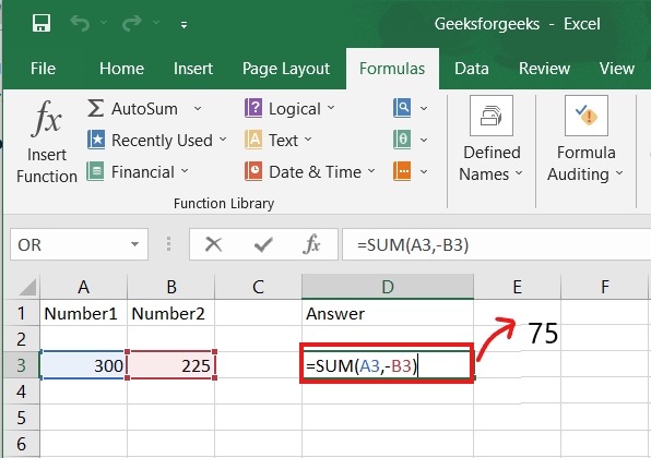
2. SUBTRACTION:
To use the subtraction formula in Excel, enter the cells you want to subtract in the format =SUM (A1, -B1). This will subtract a cell from the SUM formula by appending a negative sign before the cell being subtracted.
For example, if A3 was 300 and B3 was 225, =SUM(A1, -B1) would perform 300 + -225, returning a value of 75 in D3 cell.
3. MULTIPLICATION:
In Excel, enter the cells to be multiplied in the format =A3*B3 to perform the multiplication formula. An asterisk is used in this formula to multiply cell A3 by cell B3.
For example, if A3 was 300 and B3 was 225, =A1*B1 would return a value of 67500.
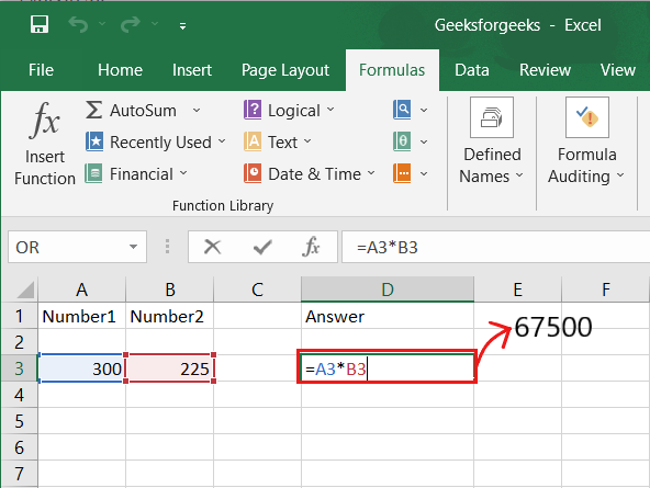
Highlight an empty cell in an Excel spreadsheet to multiply two or more values. Then, in the format =A1*B1…, enter the values or cells you want to multiply together. The asterisk effectively multiplies each value in the formula.
To return your desired product, press Enter. Take a look at the screenshot above to see how this looks.
4. DIVISION:
To use the division formula in Excel, enter the dividing cells in the format =A3/B3. This formula divides cell A3 by cell B3 with a forward slash, “/.”
For example, if A3 was 300 and B3 was 225, =A3/B3 would return a decimal value of 1.333333333.
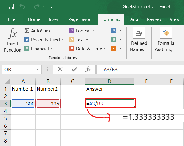
Division in Excel is one of the most basic functions available. To do so, highlight an empty cell, enter an equals sign, “=,” and then the two (or more) values you want to divide, separated by a forward slash, “/.” The output should look like this: =A3/B3, as shown in the screenshot above.
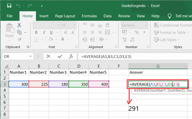
5. AVERAGE:
The AVERAGE function finds an average or arithmetic mean of numbers. to find the average of the numbers type = AVERAGE(A3.B3,C3….) and press ‘Enter’ it will produce average of the numbers in the cell.
For example, if A3 was 300, B3 was 225, C3 was 180, D3 was 350, E3 is 400 then =AVERAGE(A3,B3,C3,D3,E3) will produce 291.
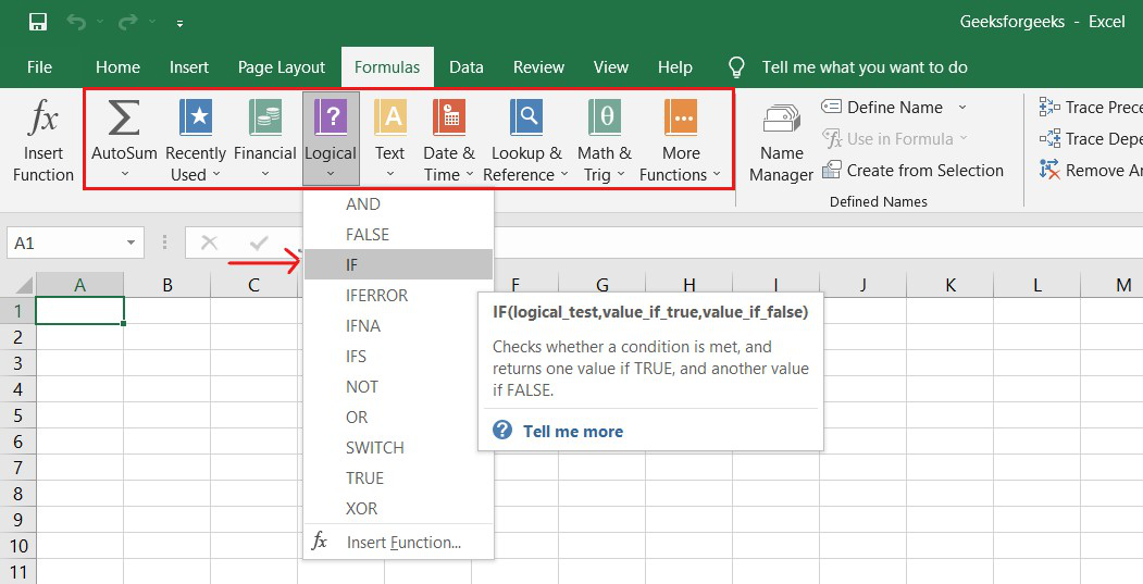
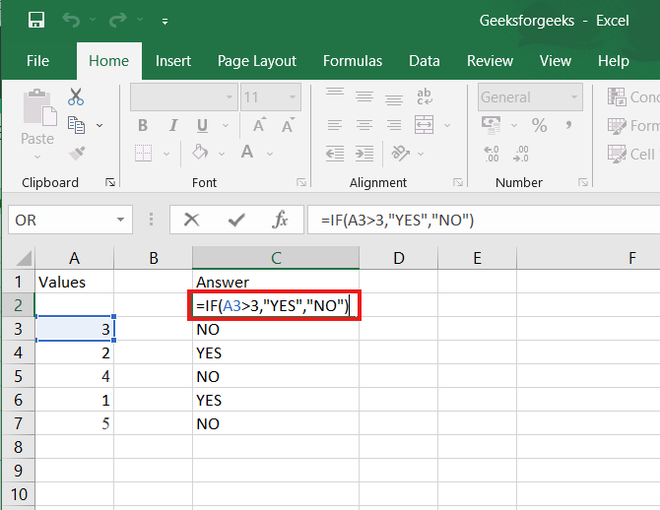
6. IF formula:
In Excel, the IF formula is denoted as =IF(logical test, value if true, value if false). This lets you enter a text value into a cell “if” something else in your spreadsheet is true or false.
For example, You may need to know which values in column A are greater than three. Using the =IF formula, you can quickly have Excel auto-populate a “yes” for each cell with a value greater than 3 and a “no” for each cell with a value less than 3.
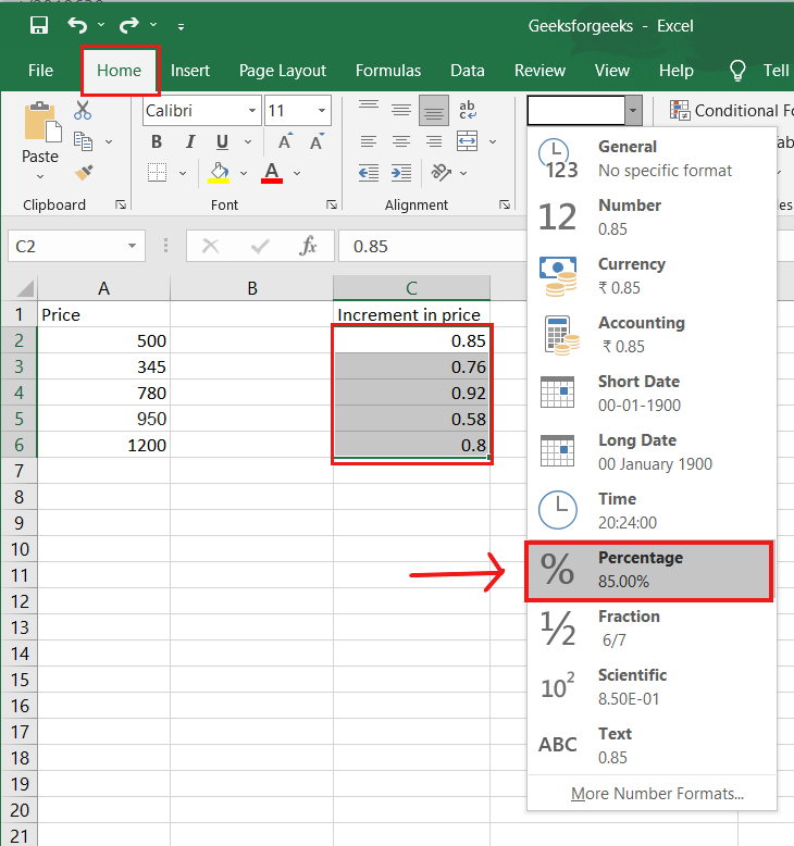
7. PERCENTAGE:
To use the percentage formula in Excel, enter the cells you want to calculate the percentage for in the format =A1/B1. To convert the decimal value to a percentage, select the cell, click the Home tab, and then select “Percentage” from the numbers dropdown.
There isn’t a specific Excel “formula” for percentages, but Excel makes it simple to convert the value of any cell into a percentage so you don’t have to calculate and reenter the numbers yourself.
The basic setting for converting a cell’s value to a percentage is found on the Home tab of Excel. Select this tab, highlight the cell(s) you want to convert to a percentage, and then select Conditional Formatting from the dropdown menu (this menu button might say “General” at first). Then, from the list of options that appears, choose “Percentage.” This will convert the value of each highlighted cell into a percentage. This feature can be found further down.
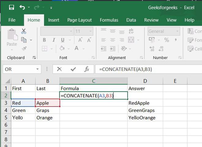
8. CONCATENATE:
CONCATENATE is a useful formula that combines values from multiple cells into the same cell.
For example , =CONCATENATE(A3,B3) will combine Red and Apple to produce RedApple.
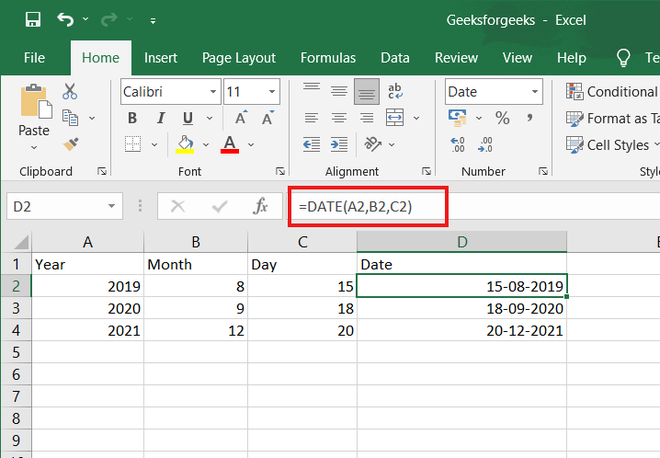
9. DATE:
DATE is the Excel DATE formula =DATE(year, month, day). This formula will return a date corresponding to the values entered in the parentheses, including values referred to from other cells.. For example, if A2 was 2019, B2 was 8, and C1 was 15, =DATE(A1,B1,C1) would return 15-08-2019.
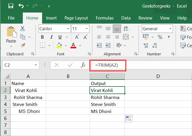
10. TRIM:
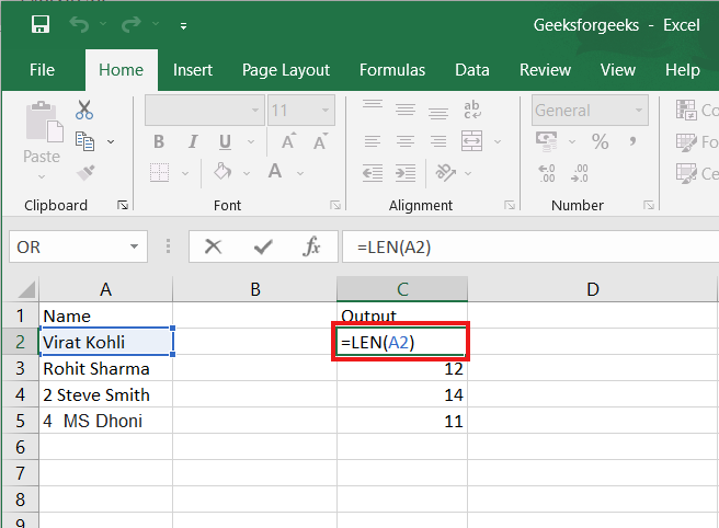
The TRIM formula in Excel is denoted =TRIM(text). This formula will remove any spaces that have been entered before and after the text in the cell. For example, if A2 includes the name ” Virat Kohli” with unwanted spaces before the first name, =TRIM(A2) would return “Virat Kohli” with no spaces in a new cell.
11. LEN:
LEN is the function to count the number of characters in a specific cell when you want to know the number of characters in that cell. =LEN(text) is the formula for this. Please keep in mind that the LEN function in Excel counts all characters, including spaces:
For example,=LEN(A2), returns the total length of the character in cell A2 including spaces.