
Change the column width or row height in Excel
You can manually adjust the column width or row height or automatically resize columns and rows to fit the data.

Note: The boundary is the line between cells, columns, and rows. If a column is too narrow to display the data, you will see ### in the cell.
Resize rows
-
Select a row or a range of rows.
-
On the Home tab, select Format > Row Width (or Row Height).
-
Type the row width and select OK.
Resize columns
-
Select a column or a range of columns.
-
On the Home tab, select Format > Column Width (or Column Height).
-
Type the column width and select OK.
Automatically resize all columns and rows to fit the data
-
Select the Select All button
 at the top of the worksheet, to select all columns and rows.
 -
Double-click a boundary. All columns or rows resize to fit the data.
 at the top of the worksheet, to select all columns and rows.
Need more help?
You can always ask an expert in the Excel Tech Community or get support in the Answers community.
See Also
Insert or delete cells, rows, and columns
Need more help?
Want more options?
Explore subscription benefits, browse training courses, learn how to secure your device, and more.
Communities help you ask and answer questions, give feedback, and hear from experts with rich knowledge.
Adding a column in Excel means inserting a new column to the existing dataset. Besides inserting, one may need to delete, hide, unhide, and move rows or columns. Such modifications help in structuring and organizing the dataset. As a result, it is essential to be aware of the techniques related to these alterations.
For example, while preparing a consolidated balance sheet, Mr. X realizes that the data related to the previous year is missing. To include this data, he wants to insert a new column. Here, the method of inserting a column comes into use.
Excel provides different ways of performing actions on a dataset. This article discusses the most appropriate and effective methods of working with data. It covers the following aspects: –
- Insert Excel columns (alternate methods and shortcuts)
- Delete columns and rows
- Hide and unhide rows or columns
- Move rows or columns
Apart from inserting columns in Excel, the remaining topics have been covered in brief.
Table of contents
- How to Add/Insert Columns in Excel?
- Example #1–Add Columns in Excel
- Example #2–Alternate Method to Insert Rows and Columns in Excel
- Example #3–Hide and Unhide Columns & Rows in Excel
- Example #4–Move Rows or Columns in Excel
- Shortcuts to Insert Columns in Excel
- Frequently Asked Questions
- Recommended Articles
How to Add/Insert Columns in Excel?
Below are some examples through which you may learn how to add and insert columns in Excel.
Example #1–Add Columns in Excel
The following table shows the first and the last names in columns A and B, respectively. We want to insert a new column (column B) between these names, which will display the middle name.

The steps to insert a new column (column B) between two existing columns (columns A and B) are listed as follows:
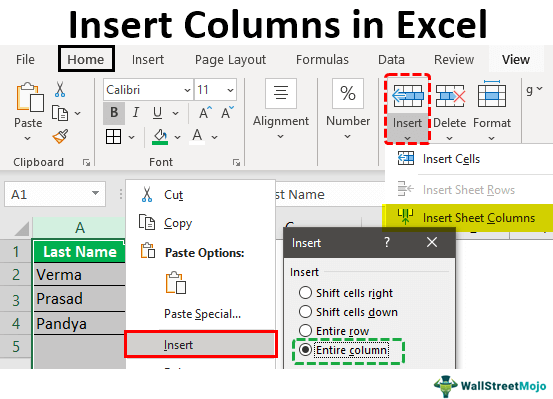
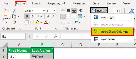
Step 1: Select any cell of column B. Alternatively, one can also select column B, as shown in the following image. Further, click the “Insert” drop-down from the “Home” tab of the Excel ribbonThe ribbon is an element of the UI (User Interface) which is seen as a strip that consists of buttons or tabs; it is available at the top of the excel sheet. This option was first introduced in the Microsoft Excel 2007.read more. Finally, select “Insert Sheet Columns.”
Note: To select a column, click its label or header on top.
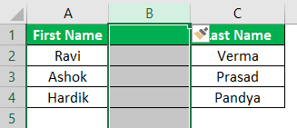
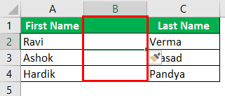
Step 2: A new column (column B) is inserted between the columns containing the first and the last names. As a result, the data (last name) of the previous column B (shown in step 1) now shifts to column C.
Note: Excel inserts a column immediately preceding the column of the selected cell. Hence, one must always choose a cell accordingly. If a column is selected, Excel inserts a column preceding it.
Example #2–Alternate Method to Insert Rows and Columns in Excel
Working on the data of example #1, we need to insert a middle name column using the following methods:
a) Select and right-click a cell
b) Select and right-click a column
a) The steps for inserting a column after selecting and right-clicking a cell are listed as follows:
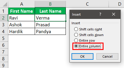
Step 1: Select any cell of column B. This is because a column preceding column B is to be inserted. Right-click the selection and choose “insert,” as shown in the following image.
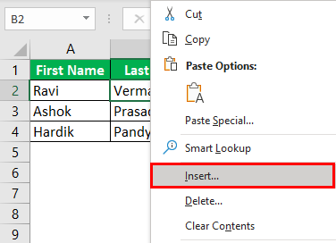
Step 2: The “Insert” dialog box appears. Select “Entire column” to insert a new column.
Note: For inserting a new row, select “Entire row.”
Step 3: A new column (column B) for typing middle names has been inserted.
b) The steps for inserting a column after selecting and right-clicking a column are listed as follows:
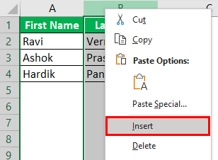
Step 1: Select the entire column B. That is because a column preceding column B is to be inserted. Right-click the selection and choose “Insert,” as shown in the following image.
Step 2: A new column B is inserted. The same has been shown under step 3 of method a.
Note: Select the entire row preceding which a new row is inserted for inserting rows. Right-click the selection and choose “Insert.” The same is shown in the following image.

Example #3–Hide and Unhide Columns & Rows in Excel
Working on the data of example #1, we want to perform the following tasks:
a) Hide columns A and B or rows 3 and 4 by right-clicking
b) Hide column A by using the “format” drop-down
c) Unhide columns B and C by right-clicking
a) The steps to hide the columns A and B or rows 3 and 4 by right-clicking are listed as follows:
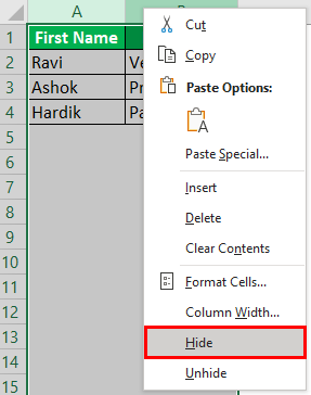
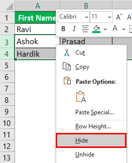
Step 1: Select columns A and B. Right-click the selection and choose “hide,” as shown in the next image.
Note 1: To select a row or column, click the row number (to the left) or the column label (on top).
Note 2: Multiple adjacent rows or columns can be selected by dragging across the row and column headings. Alternatively, hold the “Shift” key while selecting the rows or columns.
Note 3: We can select non-adjacent rows or columns by holding the “Ctrl” key while making the selections.
Step 2: Columns A and B will be hidden. Likewise, select rows 3 and 4. Right-click the selection and choose the “Hide” option from the context menu. The same is shown in the following image.
It will hide rows 3 and 4.
b) The steps to hide column A by using the “format” drop-down are listed as follows:
Step 1: Select any cell of column A. Click the “Format” drop-down under the “Home” tab of the Excel ribbon. Next, select “Hide Columns” under the “Hide & Unhide” option.
The same is shown in the following image.
Note: Alternatively, select the relevant column to be hidden. Click “Hide columns” under the “Hide & Unhide” option.
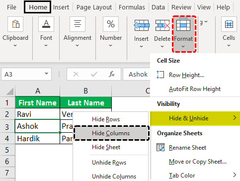
Step 2: We will hide the column of the selected cell, column A. Likewise, to hide rows, select the relevant row. Then, choose “Hide Rows” from the “Hide & Unhide” option of the “Format” drop-down.
c) The steps to unhide columns B and C by right-clicking are listed as follows:
Step 1: Select the unhidden columns (A and D) immediately before and after the hidden columns (B and C). Right-click the selection and choose “Unhide.”
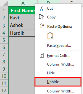
Step 2: The columns B and C will be unhidden. The dataset appears as shown in step 1 of task b.
Likewise, unhide rows by selecting the “Unhide rows” (immediately before and after the hidden rows) and clicking “Unhide” from the context menu.
Example #4–Move Rows or Columns in Excel
Working on the data of example #1, we want to move column B (last name) to precede column A (first name).
The steps to move column B are listed as follows:
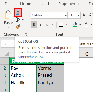
Step 1: Select column B, which is to be moved. Cut it in either of the following ways:
- Press “Ctrl+X.”
- Click the scissors icon from the “Clipboard” group of the “Home” tab.
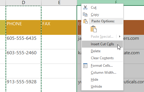
Step 2: Select column A, where the data of column B is to be pasted. Right-click the selection and choose “Insert Cut Cells.”
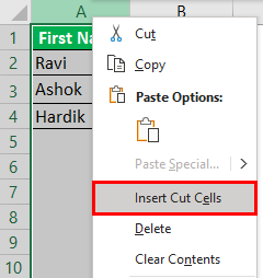
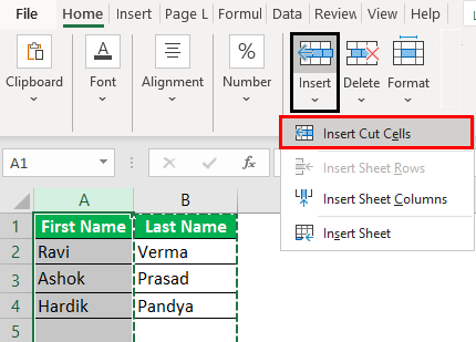
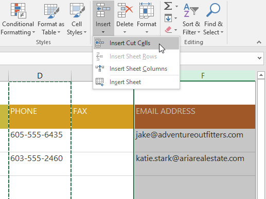
Alternatively, select “Insert Cut Cells” from the “Insert” drop-down of the “Home” tab. The same is shown in the following image.
Note: The “Insert Cut Cells” option will be visible once the selected cells have been cut.
Step 3: The data of column B is pasted into column A. Hence, the first column (column A) now contains the last names. The data of the initial column A (first name) automatically shifts to column B.
The same is shown in the following image.
Note: A row can be selected, cut, and pasted to the desired location. Select the “Insert Cut Cells” option from the “Insert” drop-down of the “Home” tab for pasting.

Shortcuts to Insert Columns in Excel
Let us go through the two shortcuts for inserting columns and rows.
a) Shortcut for inserting with the “Insert” drop-down of the “Home” tab
The excel shortcutAn Excel shortcut is a technique of performing a manual task in a quicker way.read more for inserting a row or column with the “Insert” drop-down works as follows:
- Select a cell preceding which a row or column is inserted.
- Click the “Insert” drop-down from the “Cells” group of the “Home” tab.
- Press “R” to insert a row or “C” to insert a column
A new row or column is inserted depending on the third pointer’s key.
Note: Under the “Insert” drop-down, the “R” of “insert sheet rows” and the “C” of “insert sheet columns” are underlined. Hence, these keys work as shortcuts for inserting rows and columns.
b) Shortcut for inserting with right-click
- The shortcut for inserting a row or column with right-click works as follows:
- Select a cell preceding which a row or column is inserted.
- Right-click the selection and press “I.” The “Insert” dialog box opens.
- Press “R” to insert a row or “C” to insert a column.
- Press the “Enter” key.
A new row or column is inserted depending on the third pointer’s key.
Note: If the “Insert” dialog box does not open in step 2, press the “Enter” key after pressing “I.” It opens the “Insert” dialog box.
Frequently Asked Questions
1. What does it mean to insert a column? How is it done in Excel?
Inserting a column refers to adding a new column to an existing dataset. This new column may contain additional data that can be important for the end-user.
Additionally, there is a possibility that a column has been omitted by mistake. In such cases, inserting a column will be helpful.
The steps to insert a column in Excel are listed as follows:
a. Select the column preceding which a new column is to be inserted.
b. Right-click the selection and choose “Insert” from the context menu.
It will insert the new column immediately before the selected column.
Note: To select a column, click its header (label) on top.
2. How to insert a column in Excel by using a shortcut?
Let us insert a new column E in Excel. The steps to insert a column (column E) by using a shortcut are listed as follows:
a. Select the existing column E.
b. Press the keys “Ctrl+Shift+plus sign(+)” together to insert a column.
It will insert the new column E. The data of the initial column E now shifts to column F.
Note 1: One must select a column carefully. That is because Excel inserts a column preceding the selected column.
Note 2: As an alternative to step a, one can select any cell of column E. After that, press “Ctrl+space” to select the entire column E.
3. How to insert multiple adjacent columns in Excel?
Let us insert columns D, E, and F in Excel. The steps to insert multiple columns (D, E, and F) are listed as follows:
a. Select as many columns in the existing dataset as the number of the new columns to be inserted. So, select the current columns D, E, and F.
b. Press the keys “Ctrl+Shift+plus sign(+)” together.
It will insert the blank columns D, E, and F. The initial columns D, E, and F data shift to columns G, H, and I.
Note 1: Alternative to step a: select adjacent cells of columns D, E, and F. These cells should be in one row. Further, press “Ctrl+space.” As a result, columns D, E, and F will be selected.
Note 2: To select multiple adjacent columns (in step a), drag across the column headings. Alternatively, hold the “Shift” key while selecting the columns.
Note 3: Alternative to step b: right-click the selection and choose “Insert.”
Recommended Articles
This article is a guide to Add Columns in Excel. We also discuss inserting, hiding, and moving rows and columns in Excel and practical examples. You may learn more about Excel from the following articles: –
- Compare Two Columns in Excel for Matches
- 3 Ways to Show Excel Negative Numbers
- Rows vs. Columns
- Move Columns in Excel

Excel Add Column (Table of Contents)
- Add Column in Excel
- How to Add Column in Excel?
- How to Modify a Column Width?
Add Column in Excel
Excel allows a user to add columns, whether left or right, of the column in the worksheet, which is called Add Column in Excel. Of course, there is more than one way to accomplish a task, as in all Microsoft programs. These instructions cover how rows and columns can be added and modified in an Excel worksheet using a keyboard shortcut and using the context menu with the right-click.
How to Add Column in Excel?
Adding a column in Excel is very easy and convenient whenever we want to add data to the table. There are different Methods to Insert or add Column which is as follows:
- Manually we can do this by just right-clicking on the selected column> then click on the insert button.
- Use Shift + Ctrl + + shortcut to add a new column in the Excel.
- Home tab >> click on Insert >> Select Insert Sheet Columns.
- We can add N number of columns in the Excel sheet; a user needs to select that many columns which number of columns he wants to insert.
Let’s understand How to Add Column in Excel with a few examples.
Example #1
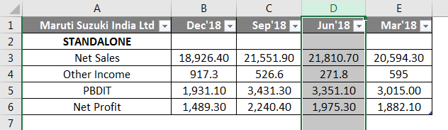
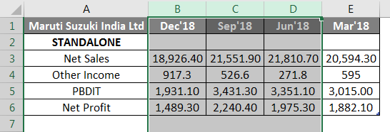
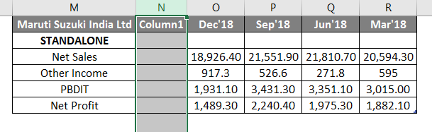
A user has a standalone book data of sales, income, PBDIT, and Profit details of each quarter of Maruti Suzuki India Pvt Ltd in sheet1.
You can download this Add a Column Excel Template here – Add a Column Excel Template
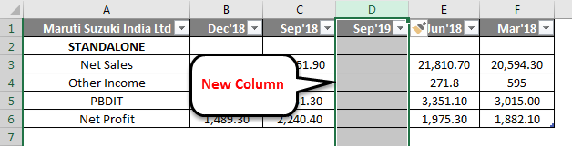
Step 1: Select the column where a user wants to add the column in the excel worksheet (The new column will be inserted to the left of the selected column, so select accordingly)
Step 2: A user has selected the D column where he wants to insert the new column.
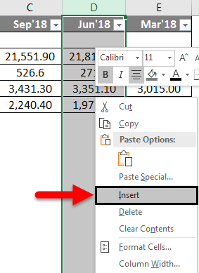
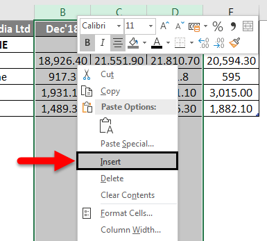
Step 3: Now Right-click and select Insert button or use shortcut Shift + Ctrl + +
Or

As we can see, as it was required to insert a new column between C and D column, in the above example, we have added a new column. So, as a result, it will move the D column data to the next column, which is E, and it will take the place of D.
Example #2
Let’s take the same data to analyze this example. A user wants to insert three columns left of the B column.
Step 1: Select B, C, and D columns where a user wants to insert new 3 columns in the worksheet (The new column is inserted to the left of the selected column, so select accordingly)
Step 2: A user has selected the B, C, and D columns where he wants to insert a new column
Step 3: Now Right-click and select Insert button or use shortcut Shift + Ctrl + +
Or
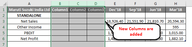
As we can see, as it was required to insert a new column left of the B, C, and D column, we added a new column in the above example. As a result, it will move B, C, and D column data to the next column, which are E, F, and G; it will take the place of the B, C, and D column.
Example #3
Step 1: Go to Worksheet >> Select the column’s heading where a user wants to insert a new column.
Step 2: Click on the Insert button.
Step 3: One drop-down will be open; click on the Insert Sheet Columns.
As the user wants to use the Insert toolbar to insert a new column, as in the above example, it added.
Example #4
The user can insert a new column in any version of Excel; in the above examples, we can see that we had selected one or more columns in the worksheet then >Right click on the selected column> then clicked on the Insert button.
To add a new column in the excel worksheet.
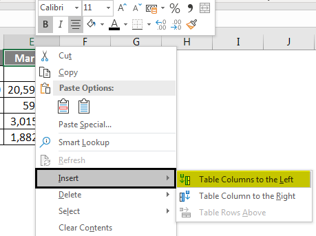
Click in a cell to the left or right of where you want to add a column. If the user wants to add a column to the left of the cell, then follow the below process:
- Click on Table Columns to the Left from the Insert option.
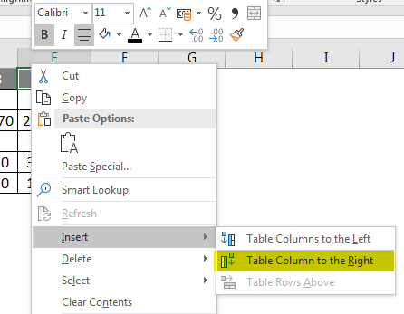
And if a user wants to insert the column to the right of the cell, then follow the below process:
- Click on Table Columns to the Right from the Insert option.
How to Modify a Column Width?
A user can modify the width of any column. Let’s take an example as some of the content in column A cannot be displayed. We can make all this content visible by changing the width of column A.
Step 1: Position the mouse over the column line in the column heading to the Black Cross. (As shown below)
Step 2: Click, hold and drag the mouse to increase or decrease the column width.
Step 3: Release the mouse. The column width will be changed.
A user can auto fit the width of the column. The AutoFit feature will allow you to set a column’s width to fit its content automatically.
Step1: Position the mouse over the column line in the column heading to the Black Cross.
Step2: Double-click the mouse. The column width will be changed automatically to fit the content.
Things to Remember About Add a Column in Excel
- The user needs to select that column where the user wants to insert the new column.
- By default, every row and column have the same height and width, but a user can modify the width of the column and the height of the row.
- The user can insert multiple columns at a time.
- You can also AutoFit the width for several columns at the same time. Simply select the columns you want to AutoFit, and then select the AutoFit Column Width command from the Format drop-down menu on the Home. This method can also be used for row height.
- All the rules will also be applied for rows, as applied to column insertion.
- Excel allows the user to wrap text and merging cells.
- For deleting also, we can go to Home Tab >> Delete >> Delete Sheet Columns; either we can select the column which we want to delete or >> Right Click >> click on Delete.
- After adding the insert column, all the data will be shifted to the right side after that column.
Recommended Articles
This is a guide to add a column in excel. Here we have discussed How to Add a column in excel by using different methods and How to modify a column in Excel along with practical examples and a downloadable excel template. You can also go through our other suggested articles –
- COLUMNS Formula in Excel
- Switching Columns in Excel
- Excel COLUMN to Number
- Freeze Columns in Excel
Lesson 6: Modifying Columns, Rows, and Cells
/en/excel/cell-basics/content/
Introduction
By default, every row and column of a new workbook is set to the same height and width. Excel allows you to modify column width and row height in different ways, including wrapping text and merging cells.
Optional: Download our practice workbook.
Watch the video below to learn more about modifying columns, rows, and cells.
To modify column width:
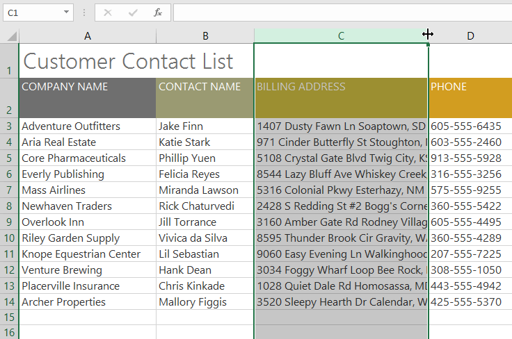
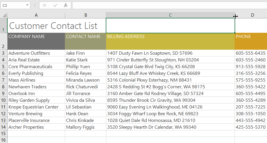
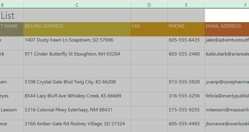
In our example below, column C is too narrow to display all of the content in these cells. We can make all of this content visible by changing the width of column C.
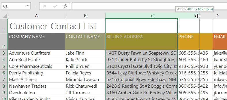
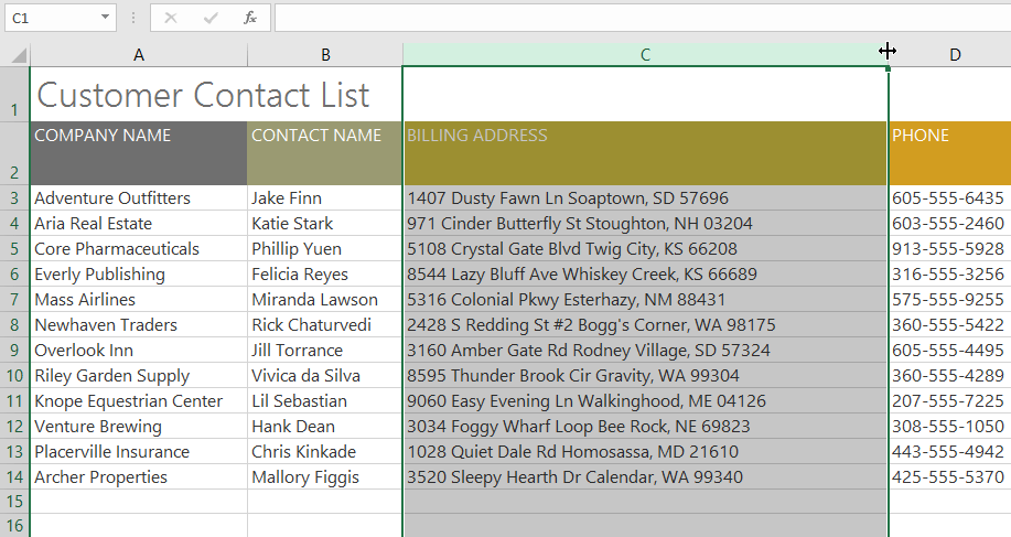
- Position the mouse over the column line in the column heading so the cursor becomes a double arrow.

- Click and drag the mouse to increase or decrease the column width.

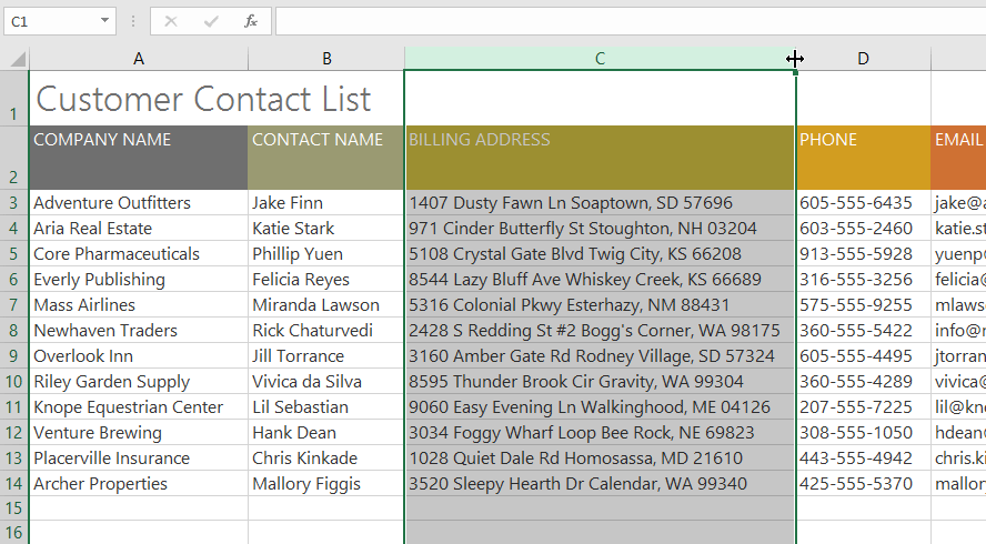
- Release the mouse. The column width will be changed.

With numerical data, the cell will display pound signs (#######) if the column is too narrow. Simply increase the column width to make the data visible.
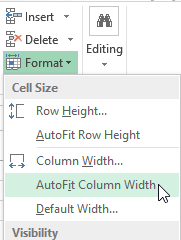
To AutoFit column width:
The AutoFit feature will allow you to set a column’s width to fit its content automatically.
- Position the mouse over the column line in the column heading so the cursor becomes a double arrow.

- Double-click the mouse. The column width will be changed automatically to fit the content.

You can also AutoFit the width for several columns at the same time. Simply select the columns you want to AutoFit, then select the AutoFit Column Width command from the Format drop-down menu on the Home tab. This method can also be used for row height.
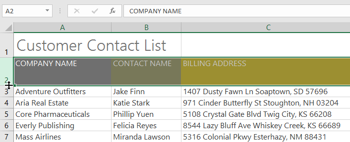
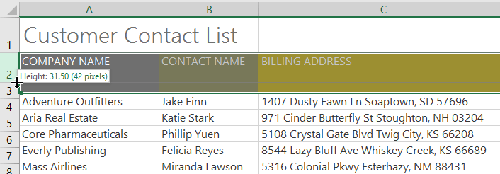
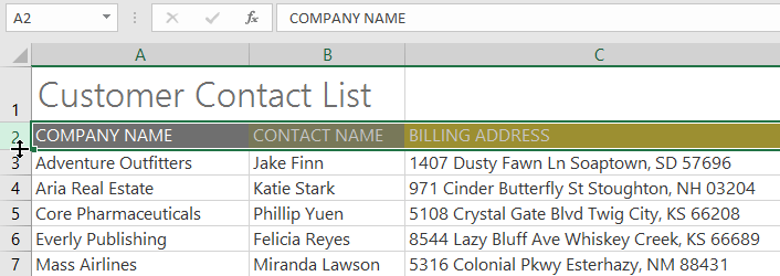
To modify row height:
- Position the cursor over the row line so the cursor becomes a double arrow.
- Click and drag the mouse to increase or decrease the row height.
- Release the mouse. The height of the selected row will be changed.
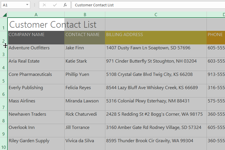
To modify all rows or columns:
Instead of resizing rows and columns individually, you can modify the height and width of every row and column at the same time. This method allows you to set a uniform size for every row and column in your worksheet. In our example, we will set a uniform row height.
- Locate and click the Select All button just below the name box to select every cell in the worksheet.
- Position the mouse over a row line so the cursor becomes a double arrow.
- Click and drag the mouse to increase or decrease the row height, then release the mouse when you are satisfied. The row height will be changed for the entire worksheet.

Inserting, deleting, moving, and hiding
After you’ve been working with a workbook for a while, you may find that you want to insert new columns or rows, delete certain rows or columns, move them to a different location in the worksheet, or even hide them.
To insert rows:
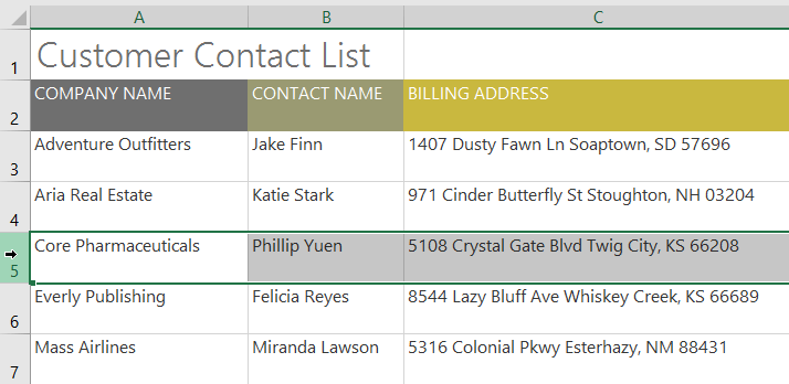
- Select the row heading below where you want the new row to appear. In this example, we want to insert a row between rows 4 and 5, so we’ll select row 5.
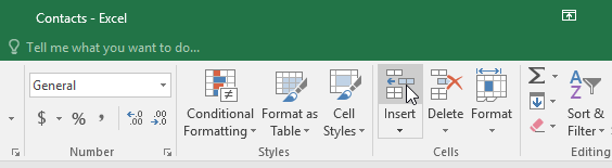
- Click the Insert command on the Home tab.
- The new row will appear above the selected row.
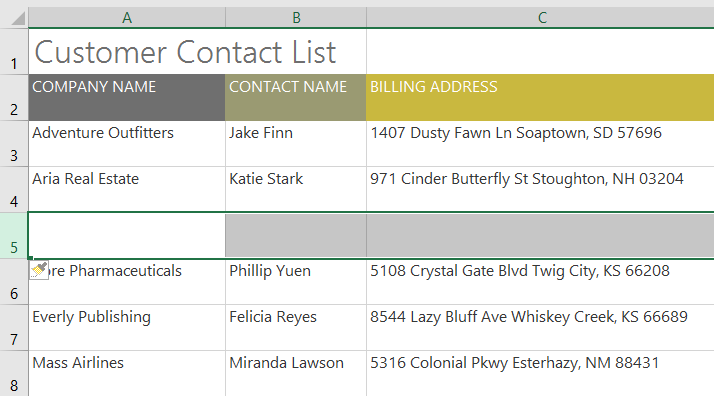
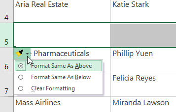
When inserting new rows, columns, or cells, you will see a paintbrush icon next to the inserted cells. This button allows you to choose how Excel formats these cells. By default, Excel formats inserted rows with the same formatting as the cells in the row above. To access additional options, hover your mouse over the icon, then click the drop-down arrow.
To insert columns:
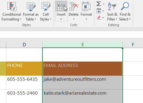
- Select the column heading to the right of where you want the new column to appear. For example, if you want to insert a column between columns D and E, select column E.
- Click the Insert command on the Home tab.
- The new column will appear to the left of the selected column.
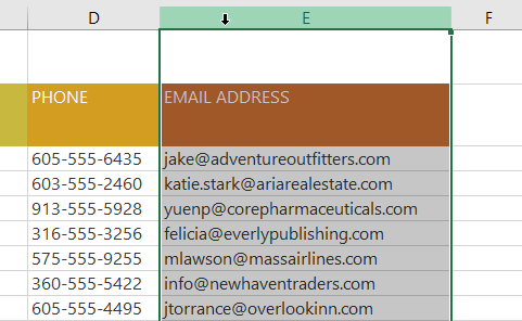
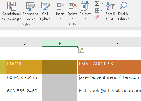
When inserting rows and columns, make sure to select the entire row or column by clicking the heading. If you select only a cell in the row or column, the Insert command will only insert a new cell.
To delete a row or column:
It’s easy to delete a row or column that you no longer need. In our example we’ll delete a row, but you can delete a column the same way.
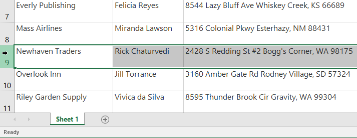
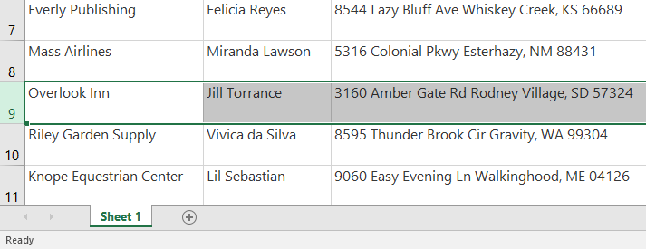
- Select the row you want to delete. In our example, we’ll select row 9.
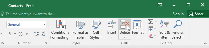
- Click the Delete command on the Home tab.
- The selected row will be deleted, and those around it will shift. In our example, row 10 has moved up, so it’s now row 9.
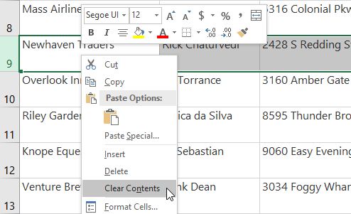
It’s important to understand the difference between deleting a row or column and simply clearing its contents. If you want to remove the content from a row or column without causing others to shift, right-click a heading, then select Clear Contents from the drop-down menu.
To move a row or column:
Sometimes you may want to move a column or row to rearrange the content of your worksheet. In our example we’ll move a column, but you can move a row in the same way.
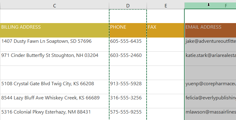
- Select the desired column heading for the column you want to move.
- Click the Cut command on the Home tab, or press Ctrl+X on your keyboard.
- Select the column heading to the right of where you want to move the column. For example, if you want to move a column between columns E and F, select column F.
- Click the Insert command on the Home tab, then select Insert Cut Cells from the drop-down menu.
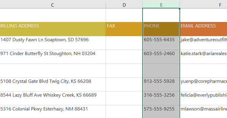
- The column will be moved to the selected location, and the columns around it will shift.
You can also access the Cut and Insert commands by right-clicking the mouse and selecting the desired commands from the drop-down menu.
To hide and unhide a row or column:
At times, you may want to compare certain rows or columns without changing the organization of your worksheet. To do this, Excel allows you to hide rows and columns as needed. In our example we’ll hide a few columns, but you can hide rows in the same way.
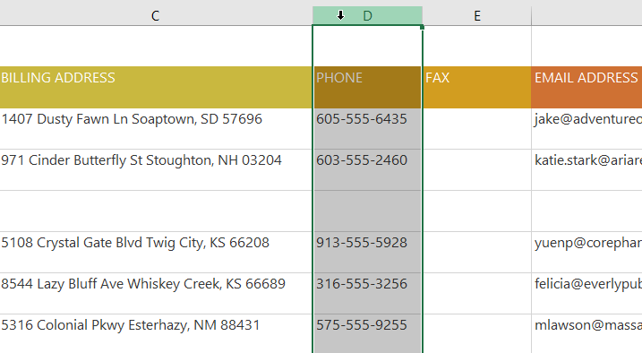
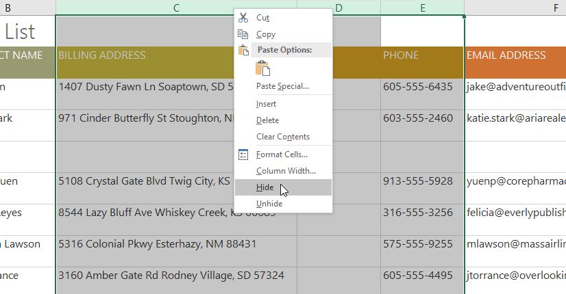
- Select the columns you want to hide, right-click the mouse, then select Hide from the formatting menu. In our example, we’ll hide columns C, D, and E.

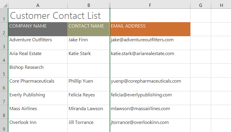
- The columns will be hidden. The green column line indicates the location of the hidden columns.
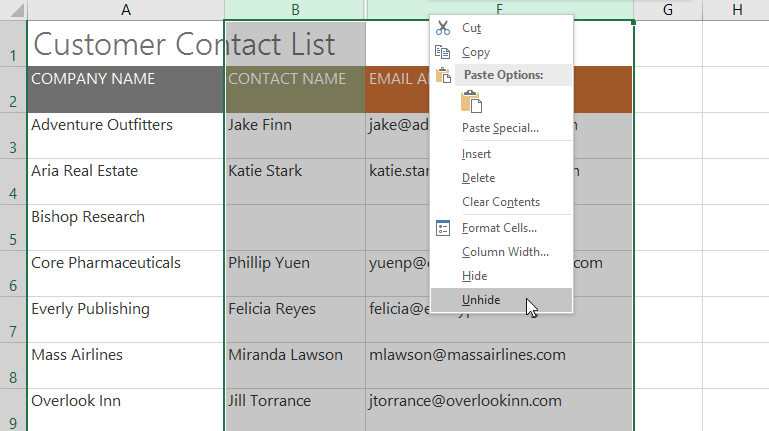
- To unhide the columns, select the columns on both sides of the hidden columns. In our example, we’ll select columns B and F. Then right-click the mouse and select Unhide from the formatting menu.
- The hidden columns will reappear.

Wrapping text and merging cells
Whenever you have too much cell content to be displayed in a single cell, you may decide to wrap the text or merge the cell rather than resize a column. Wrapping the text will automatically modify a cell’s row height, allowing cell contents to be displayed on multiple lines. Merging allows you to combine a cell with adjacent empty cells to create one large cell.
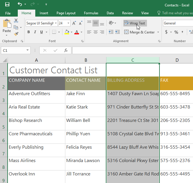
To wrap text in cells:
- Select the cells you want to wrap. In this example, we’ll select the cells in column C.
- Click the Wrap Text command on the Home tab.
- The text in the selected cells will be wrapped.
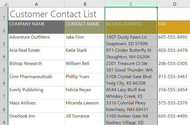
Click the Wrap Text command again to unwrap the text.
To merge cells using the Merge & Center command:
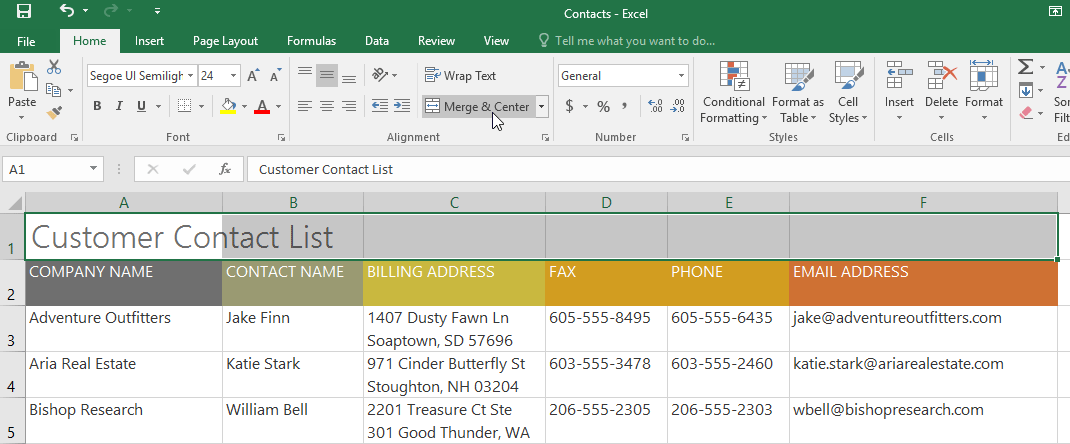
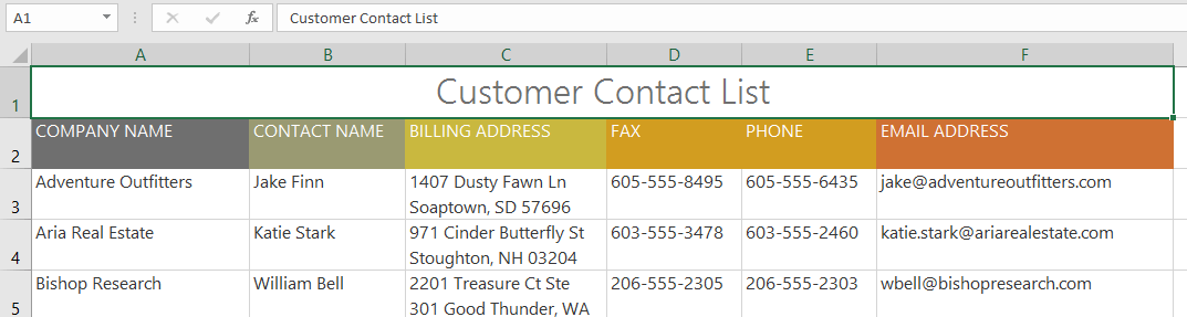
- Select the cell range you want to merge. In our example, we’ll select A1:F1.
- Click the Merge & Center command on the Home tab. In our example, we’ll select the cell range A1:F1.

- The selected cells will be merged, and the text will be centered.

To access additional merge options:
If you click the drop-down arrow next to the Merge & Center command on the Home tab, the Merge drop-down menu will appear.
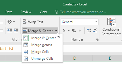
From here, you can choose to:
- Merge & Center: This merges the selected cells into one cell and centers the text.
- Merge Across: This merges the selected cells into larger cells while keeping each row separate.
- Merge Cells: This merges the selected cells into one cell but does not center the text.
- Unmerge Cells: This unmerges selected cells.
Be careful when using this feature. If you merge multiple cells that all contain data, Excel will keep only the contents of the upper-left cell and discard everything else.
Centering across selection
Merging can be useful for organizing your data, but it can also create problems later on. For example, it can be difficult to move, copy, and paste content from merged cells. A good alternative to merging is to Center Across Selection, which creates a similar effect without actually combining cells.
Watch the video below to learn why you should use Center Across Selection instead of merging cells.
To use Center Across Selection:
- Select the desired cell range. In our example, we’ll select A1:F1. Note: If you already merged these cells, you should unmerge them before continuing to step 2.
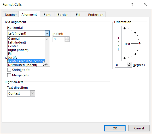
- Click the small arrow in the lower-right corner of the Alignment group on the Home tab.
- A dialog box will appear. Locate and select the Horizontal drop-down menu, select Center Across Selection, then click OK.
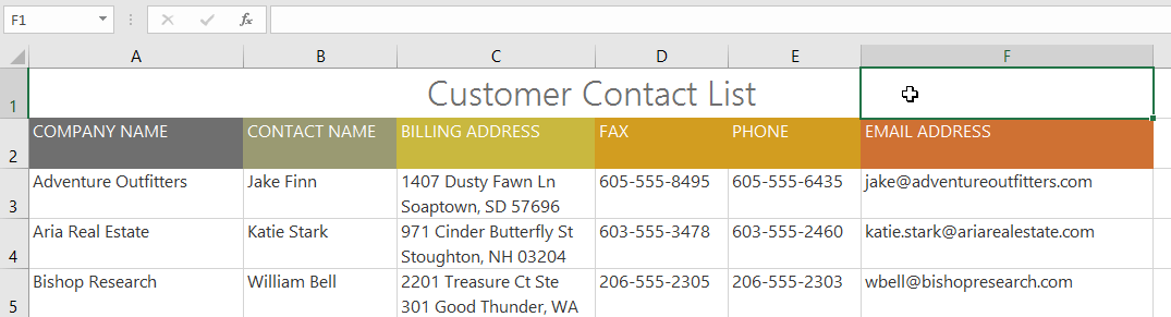
- The content will be centered across the selected cell range. As you can see, this creates the same visual result as merging and centering, but it preserves each cell within A1:F1.

Challenge!
- Open our practice workbook.
- Autofit Column Width for the entire workbook.
- Modify the row height for rows 3 to 14 to 22.5 (30 pixels).
- Delete row 10.
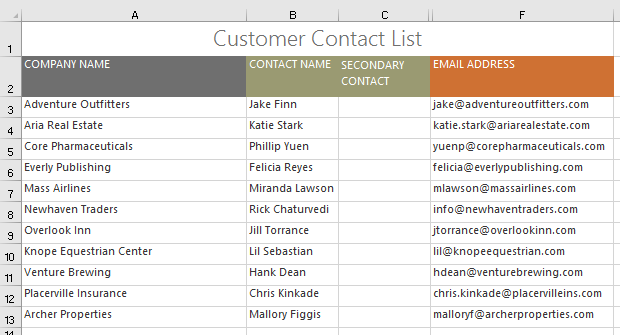
- Insert a column to the left of column C. Type SECONDARY CONTACT in cell C2.
- Make sure cell C2 is still selected and choose Wrap Text.
- Merge and Center cells A1:F1.
- Hide the Billing Address and Phone columns.
- When you’re finished, your workbook should look something like this:
/en/excel/formatting-cells/content/
A neat looking worksheet is always better than a shabby and unorganized one. You can tell if a sheet has been handled repeatedly by different people by just one look at it.
You will find it unorganized and shabby, often with rows and columns of varying sizes. Nobody likes that!
Maybe you were the one destined to put the sheet back in shape and make it nice and neat with trimmed cells that are evenly sized! In this Excel tutorial, we will help you do just that.
We will show you how you can set the column width and row height of all your cells so that they are all the same size. We will also show you how you can make sure that all the cells are well fitted around the content for added neatness.
In the end, we will show you how you can speed up this process by using simple VBA macro codes.
Setting the Column Width and Row Height of All Cells to a Specific Size
When you open a fresh Excel worksheet, you will always find the cells to be of a specific width and height by default. The default row height is 15 and the default column width is 8.43.
However, as you work on these cells, the heights and widths of the cells keep expanding to accommodate the contents of your cells.
In the end, what you get is a hodgepodge of cells of varying heights and widths.
Giving these cell sizes some uniformity though is quite easy. Here’s how you can achieve this.
If you want to resize your entire worksheet, do the following:
- Click on the ‘Select All’ button on the top-left of the Excel window.

- Set the Column width for all the cells. Right-click on any column header. Select ‘Column Width’ from the popup menu. Enter the size to which you want to set all the columns.
- Set the Row height for all the cells. Right-click on any row, select ‘Row Height’ from the popup menu. Enter the size to which you want to set all the rows.

That’s all. You will get all your cells uniformly adjusted to your required size.

Setting the Column Width and Row Height of Selected Cells to a Specific Size
If you want to resize only selected cells, do the following:
- Drag and select all your required cells. If there are a lot of cells that you need to select, click on the cell at the top left corner of your required selection, then pressing down on the SHIFT key, click on the cell at the bottom right corner of your required selection.
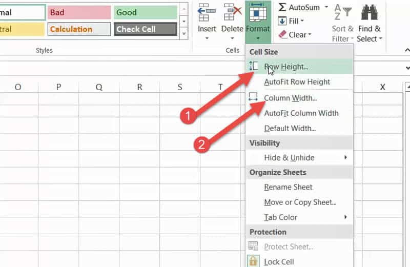
- Set the column width for the selected cells. Under the Home tab, select ‘Format’ (from the Cells group). Select ‘Column Width’ and enter the size to which you want to set all the columns in the small ‘Column Width’ window that appears.
- Set the row height for the selected cells. Under the Home tab, select ‘Format’ (from the Cells group). Select ‘Row Height’ and enter the size to which you want to set all the columns in the small ‘Row Height’ window that appears.
Your selected cells will now be equally resized to your requirement.
Applying the Same Column Width and Row Height by Using a Mouse
- Apply the same column width by selecting the column headers of all the cells you want to adjust.
- Drag the boundary of any one of the selected column headers to the width you like. When you release the mouse button, you will find all the other selected columns resized to the same width.

- Similarly, you can apply the same row height by selecting the row headers of all the cells you want to adjust.
- Drag the boundary of any one of the selected row headers to the height you like. When you release the mouse button, you will find all the other selected rows resized to the same height.

Changing the Column Width and Row Height to Auto-fit the Contents
In case you want to further make your sheet look neat, you can adjust the cell sizes to the height/ width of the cell with the highest height/ width.
- Select the column headers of the cells you want to adjust.
- Double click the boundary of any one of the selected column headers. You will find all the selected columns adjusted to fit the contents of the widest cell in each column.
- Similarly, select the row headers of the cells you want to adjust
- Double click the boundary of any one of the selected row headers. You will find all the selected rows adjusted to fit the contents of the cell with the most height in each row.
Using VBScript
If you are comfortable using VBScript, you can easily speed up the above processes by copying and pasting a short script into your developer window.
- Select the rows and columns that you want to adjust.
- From the Developer Menu Ribbon, select Visual Basic.
- Once your VBA window opens, Click Insert->Module. Now you can start adding your code.
Using VBScript to Set the Selected Cells to a Specific Size
Let us assume that you want to set all the selected cells to a column width of 10 and a row height of 20.
You can then copy and paste the following lines to your Developer window:
Sub makeequalsize()
Selection.ColumnWidth = 10
Selection.RowHeight = 20
End Sub
You can also choose to specify the range of cells that you want to set to a specific size.
For example, if you want to set the size for the range A2 to G12, you can use the following code:
Sub makeequalsize()
Range("A2:G12").ColumnWidth = 10
Range("A2:G12").RowHeight = 20
End Sub
Note: You can replace the column width and row height according to your preference.
Using VBScript to Set the Selected Cells to the Same Size as a Specific Cell
If you have a reference cell with the perfect size that you want to copy to all other cells in your selection, say cell B5, then copy and paste the following lines:
Sub makeequalsize()
Selection.ColumnWidth = Columns("B").ColumnWidth
Selection.RowHeight = Rows("5").RowHeight
End Sub
You can also choose to specify the range of cells that you want to set to the size of a particular cell.
For example, if you want to set the size for the range A2 to G12 to the size of cell B5, you can use the following code:
Sub makeequalsize()
Range("A2:G12").ColumnWidth = Columns("B").ColumnWidth
Range("A2:G12").RowHeight = Rows("5").RowHeight
End Sub
Note: You can replace the column name “B” and row number “5” with the corresponding column name and row number of your preferred cell.
Using VBScript to Auto-fit the Contents of All Selected Cells
To adjust the cell sizes to the height/ width of the cell with the highest height/ width, you can use AutoFit as follows:
To autofit the column width of the selected cells, copy-paste the following lines:
Sub autofitColumns()
Selection.Columns.AutoFit
End Sub
To autofit the row height of selected cells, copy-paste the following lines:
Sub autofitRows()
Selection.Rows.AutoFit
End Sub
To autofit both, you can combine the two commands as follows:
Sub autofitAllCells()
Selection.Columns.AutoFit
Selection.Rows.AutoFit
End Sub
Conclusion
In this tutorial, you saw how you can adjust cell sizes to make your worksheet look uniform and neat.
We have shown you how you can either set the cells to a specific height and width or adjust the height and width to match that of a specific cell.
In the end, we also showed how you can use VBA Script to programmatically and quickly get this done so that you can get this done for multiple sheets quickly.
Other Excel tutorials you may find useful:
- How to Find Merged Cells in Excel
- How to Subtract Multiple Cells from One Cell in Excel
- How to Select Every Other Cell in Excel
- How to Select Alternate Columns in Excel (or every Nth Column)
- How to Set a Row to Print on Every Page in Excel
- How to Press Enter in Excel and Stay in the Same Cell?
- How to Show Ruler in Excel? (Ruler Grayed Out)
- Autofit Column Width in Excel (Shortcut)