Setting column names in excel

How to change the name of the column headers in Excel

In Microsoft Excel, the column headers are named A, B, C, and so on by default. Some users want to change the names of the column headers to something more meaningful. Unfortunately, Excel does not allow the header names to be changed.

The same applies to row names in Excel. You cannot change the row names, or numbering, but you can add your desired row names in column A for the corresponding rows.

Instead, if you want to have meaningful column header names, you can do the following.

1. Click in the first row of the worksheet and insert a new row above that first row.

• How to add or remove a cell, column, or row in Excel.

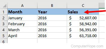
1. In the inserted row, enter the preferred name for each column.
2. To make the row of column names more noticeable, you could increase the text size, make the text bold, or add background color to the cells in that row.

After inserting the new row and adding column header names, if you want to hide the default column header names, follow the steps below to hide column and row headers.

1. In Microsoft Excel, click the File tab or the Office button in the upper-left corner.
2. In the left navigation pane, click Options.
3. In the Excel Options window, click the Advanced option in the left navigation pane.
4. Scroll down to the Display options for this worksheet section. Uncheck the box for Show row and column headers.

The column and row headers are now hidden. To display them again, re-check the box in step 4 above.

Источник

Create and format tables

Create and format a table to visually group and analyze data.

Note: Excel tables shouldn’t be confused with the data tables that are part of a suite of What-If Analysis commands ( Forecast, on the Data tab). See Introduction to What-If Analysis for more information.

Try it!

Select a cell within your data.

Select Home > Format as Table.

Choose a style for your table.

In the Create Table dialog box, set your cell range.

Mark if your table has headers.

Insert a table in your spreadsheet. See Overview of Excel tables for more information.

Select a cell within your data.

Select Home > Format as Table.

Choose a style for your table.

In the Create Table dialog box, set your cell range.

Mark if your table has headers.

To add a blank table, select the cells you want included in the table and click Insert > Table.

To format existing data as a table by using the default table style, do this:

Select the cells containing the data.

Click Home > Table > Format as Table.

If you don’t check the My table has headers box, Excel for the web adds headers with default names like Column1 and Column2 above the data. To rename a default header, double-click it and type a new name.

Note: You can’t change the default table formatting in Excel for the web.

Источник

Use the Name Manager in Excel

Use the Name Manager dialog box to work with all the defined names and table names in a workbook. For example, you may want to find names with errors, confirm the value and reference of a name, view or edit descriptive comments, or determine the scope. You can also sort and filter the list of names, and easily add, change, or delete names from one location.

To open the Name Manager dialog box, on the Formulas tab, in the Defined Names group, click Name Manager.

The Name Manager dialog box displays the following information about each name in a list box:

One of the following:

A defined name, which is indicated by a defined name icon.

A table name, which is indicated by a table name icon.

Note: A table name is the name for an Excel table, which is a collection of data about a particular subject stored in records (rows) and fields (columns). Excel creates a default Excel table name of Table1, Table2, and so on, each time you insert an Excel table. You can change a table’s name to make it more meaningful. For more information about Excel tables, see Using structured references with Excel tables.

The current value of the name, such as the results of a formula, a string constant, a cell range, an error, an array of values, or a placeholder if the formula cannot be evaluated. The following are representative examples:

«this is my string constant»

The current reference for the name. The following are representative examples:

A worksheet name, if the scope is the local worksheet level.

«Workbook,» if the scope is the global workbook level. This is the default option.

Additional information about the name up to 255 characters. The following are representative examples:

This value will expire on May 2, 2007.

Don’t delete! Critical name!

Based on the ISO certification exam numbers.

The reference for the selected name.

You can quickly edit the range of a name by modifying the details in the Refers to box. After making the change you can click Commit to save changes, or click Cancel to discard your changes.

You cannot use the Name Manager dialog box while you are changing the contents of a cell.

The Name Manager dialog box does not display names defined in Visual Basic for Applications (VBA), or hidden names (the Visible property of the name is set to False).

On the Formulas tab, in the Defined Names group, click Define Name.

In the New Name dialog box, in the Name box, type the name you want to use for your reference.

Note: Names can be up to 255 characters in length.

The scope automatically defaults to Workbook. To change the name’s scope, in the Scope drop-down list box, select the name of a worksheet.

Optionally, in the Comment box, enter a descriptive comment up to 255 characters.

In the Refers to box, do one of the following:

Click Collapse Dialog (which temporarily shrinks the dialog box), select the cells on the worksheet, and then click Expand Dialog .

To enter a constant, type = (equal sign) and then type the constant value.

To enter a formula, type = and then type the formula.

Be careful about using absolute or relative references in your formula. If you create the reference by clicking on the cell you want to refer to, Excel will create an absolute reference, such as «Sheet1!$B$1». If you type a reference, such as «B1», it is a relative reference. If your active cell is A1 when you define the name, then the reference to «B1» really means «the cell in the next column». If you use the defined name in a formula in a cell, the reference will be to the cell in the next column relative to where you enter the formula. For example, if you enter the formula in C10, the reference would be D10, and not B1.

To finish and return to the worksheet, click OK.

Note: To make the New Name dialog box wider or longer, click and drag the grip handle at the bottom.

Источник

MS Excel 2016: How to Change Column Headings from Numbers to Letters

This Excel tutorial explains how to change column headings from numbers (1, 2, 3, 4) back to letters (A, B, C, D) in Excel 2016 (with screenshots and step-by-step instructions).

See solution in other versions of Excel :

Question: In Microsoft Excel 2016, my Excel spreadsheet has numbers for both rows and columns. How do I change the column headings back to letters such as A, B, C, D?

Answer: Traditionally, column headings are represented by letters such as A, B, C, D. If your spreadsheet shows the columns as numbers, you can change the headings back to letters with a few easy steps.

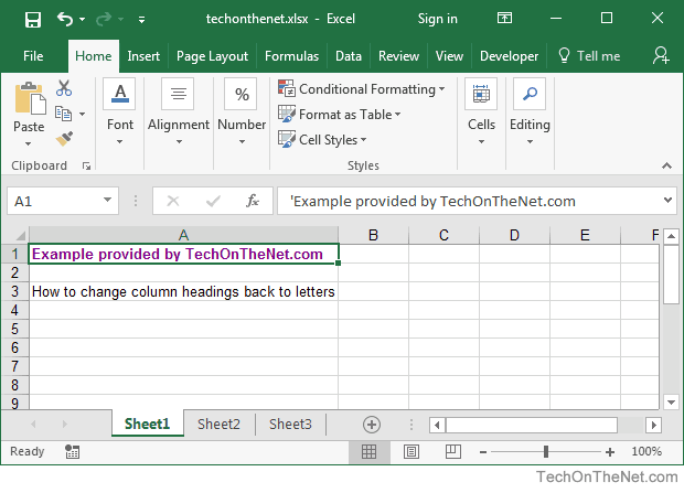
In the example below, the column headings are numbered 1, 2, 3, 4 instead of the traditional A, B, C, D values that you normally see in Excel. When the column headings are numeric values, R1C1 reference style is being displayed in the spreadsheet.

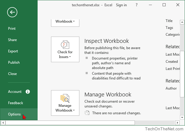
To change the column headings to letters, select the File tab in the toolbar at the top of the screen and then click on Options at the bottom of the menu.

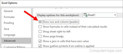
When the Excel Options window appears, click on the Formulas option on the left. Then uncheck the option called «R1C1 reference style» and click on the OK button.

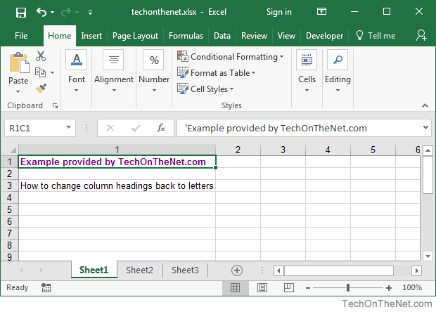
Now when you return to your spreadsheet, the column headings should be letters (A, B, C, D) instead of numbers (1, 2, 3, 4).

Источник

Columns and rows are labeled numerically in Excel

Symptoms

Your column labels are numeric rather than alphabetic. For example, instead of seeing A, B, and C at the top of your worksheet columns, you see 1, 2, 3, and so on.

Cause

This behavior occurs when the R1C1 reference style check box is selected in the Options dialog box.

Resolution

To change this behavior, follow these steps:

1. Start Microsoft Excel.
2. On the Tools menu, click Options.
3. Click the Formulas tab.
4. Under Working with formulas, click to clear the R1C1 reference style check box (upper-left corner), and then click OK.

If you select the R1C1 reference style check box, Excel changes the reference style of both row and column headings, and cell references from the A1 style to the R1C1 style.

More information

A1 Reference Style vs. R1C1 Reference Style

The A1 Reference Style

By default, Excel uses the A1 reference style, which refers to columns as letters (A through IV, for a total of 256 columns), and refers to rows as numbers (1 through 65,536). These letters and numbers are called row and column headings. To refer to a cell, type the column letter followed by the row number. For example, D50 refers to the cell at the intersection of column D and row 50. To refer to a range of cells, type the reference for the cell that is in the upper-left corner of the range, type a colon (:), and then type the reference to the cell that is in the lower-right corner of the range.

The R1C1 Reference Style

Excel can also use the R1C1 reference style, in which both the rows and the columns on the worksheet are numbered. The R1C1 reference style is useful if you want to compute row and column positions in macros. In the R1C1 style, Excel indicates the location of a cell with an «R» followed by a row number and a «C» followed by a column number.

References

For more information about this topic, click Microsoft Excel Help on the Help menu, type about cell and range references in the Office Assistant or the Answer Wizard, and then click Search to view the topic.

Источник