Set range for excel - Word и Excel - помощь в работе с программами

Excel VBA Set Range

To set the range in VBA is to select the cell where we want to put the required content or to move the cursor to the chosen cell. This helps us in building a code where we can choose the cell we want. If we do not set the range then it will automatically choose the current cell where the cursor is placed. Excel VBA Set Range helps us to choose the range as per user requirements.

In Excel, which is a common fact that whatever we do, contains a cell or table. Either it has numbers or words, everything goes into the cell. It becomes very important for us to know the fact that choosing a cell where we want to place or type of cell contact could be done easily. For that, we have the VBA Set Range, which helps us to put any value in any cell using VBA code where we can select the cell we want.

How to Use Set Range in VBA Excel?

We can choose a cell using a Range object and cell property in VBA. For example, if we want to choose cell A1 from any worksheet then we can use RANGE Object as shown below.

As per the syntax of RANGE Object, where it requires only Cell1, Cell2 as Range. If the number of cells are more than 1 then, instead of type cell name separated by commas we can choose colon (“:“). For example, if we want to select the cell from A1 to C5 then we can use the format as RANGE(“A1:C5”) instead of typing each cell into the Range syntax brackets.

You can download this VBA Set Range Excel Template.xlsm here – VBA Set Range Excel Template.xlsm

Example #1

We will see the example where we will select the range to put anything we want. For this, follow the below steps:

Step 1: Insert a new module inside Visual Basic Editor (VBE). Click on Insert tab > select Module.

Step 2: Write the subprocedure for VBA Set Range as shown below.

Code:

Sub VBA_SetRange()

End Sub

Step 3: Declare the variable using DIM as Range object as shown below.

Code:

Sub VBA_SetRange()

Dim MyRange As Range

End Sub

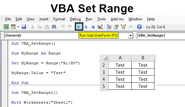
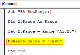
Step 4: Further setting up the range object with declared variable MyRange, we will then choose the cell which wants to include. Here those cells are A1 to B5.

Code:

Sub VBA_SetRange()

Dim MyRange As Range

Set MyRange = Range("A1:B5")

End Sub

Step 5: Let’s consider a text which we want to insert in the selected range cells as TEST as shown below.

Code:

Sub VBA_SetRange()

Dim MyRange As Range

Set MyRange = Range("A1:B5")

MyRange.Value = "Test"

End Sub

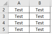
Step 6: Once done, run the code after compiling. We will see the chosen cell range A1: B5 has now text as TEST as shown below.

Example #2

There is another way to apply VBA Set Range. In this example, we will see how to set Range in different cell range and choosing the different text into the 2 or more different cell Range. For this, follow the below steps:

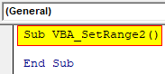
Step 1: Open a module and directly write the subprocedure for VBA Set Range.

Code:

Sub VBA_SetRange2()

End Sub

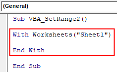
Step 2: Open With-End With loop choosing the current worksheet as Sheet1.

Code:

Sub VBA_SetRange2()

With Worksheets("Sheet1")

End With

End Sub

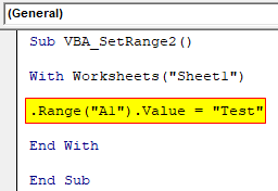
Step 3: Let’s select the cell range choosing cell A1 and putting the value in the cell range A1 as TEST as shown below.

Code:

Sub VBA_SetRange2()

With Worksheets("Sheet1")

.Range("A1").Value = "Test"

End With

End Sub

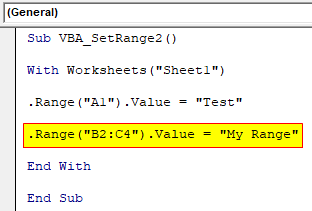
Step 4: Similar to the above-shown step, let’s choose another cell range from cell B2 to C4, choosing the value as MY RANGE as shown below.

Code:

Sub VBA_SetRange2()

With Worksheets("Sheet1")

.Range("A1").Value = "Test"

.Range("B2:C4").Value = "My Range"

End With

End Sub

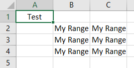
Step 5: Now we can run the code if there is no error in compilation found. We would see both the cell of the selected range A1 and cells B2:C4 as shown below with chosen texts.

Example #3

There is another simplest way to choose the VBA Set Range which is the simplest way. For this, follow the below steps:

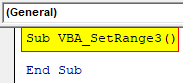
Step 1: Again open the module and write the subprocedure preferably in the name of VBA Set Range.

Code:

Sub VBA_SetRange3()

End Sub

Step 2: Choose the cell where want to set the Range. We have chosen cell A1 as shown below.

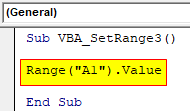
Code:

Sub VBA_SetRange3()

Range("A1").Value

End Sub

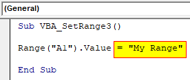
Step 3: Put the name or value which we want to insert in the select the Range cell. Here we are choosing MY RANGE again.

Code:

Sub VBA_SetRange3()

Range("A1").Value = "My Range"

End Sub

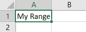
Step 4: Now if we run this code, we would see the cell A1 in the current worksheet will have the range value as MY RANGE as shown below.

Pros of VBA Set Range

It is very easy to implement and also very important to know the way to set the Range in VBA.
We can choose and set more than 1 Range value using VBA Set Range.

Things to Remember

VBA Set Range is not limited to the examples which we have seen above. There are many ways to execute VBA Set Range.
RANGE in VBA is an Object and CELLS are the property that may contain anything.
We can use CELLS properties as well to set the Range in VBA.
If we use CELLS instead of RANGE, then we would only be able to set one cell whereas with the help of the RANGE object we can choose any range or combination of cells.
It is always advised to save the Excel file in Macro enable excel format after writing the VBA Code, to avoid losing the written code in the future.

Set Range in Excel VBA

Set range in VBA means we specify a given range to the code or the procedure to execute. If we do not provide a specific range to a code, it will automatically assume the range from the worksheet with the active cell. So, it is very important in the code to have a range variable set.

After working with Excel for so many years, you must have understood that all works we do are on the worksheet. In worksheets, it is cells containing the data. So when you want to play around with data, you must be a behavior pattern of cells in worksheets. So, when the multiple cells get together, it becomes a RANGE. Therefore, to learn VBA, you should know everything about cells and ranges. So in this article, we will show you how to set the range of cells we can use for VBA codingVBA code refers to a set of instructions written by the user in the Visual Basic Applications programming language on a Visual Basic Editor (VBE) to perform a specific task.read more in detail.

Set Range in Excel VBA
- How to Access Range of Cells in Excel VBA?
- Accessing Multiple Cells & Setting Range Reference in VBA
- Things to Remember
- Recommended Articles

You are free to use this image on your website, templates, etc, Please provide us with an attribution linkArticle Link to be Hyperlinked
For eg:
Source: VBA Set Range (wallstreetmojo.com)

What is the Range Object?

Range in VBA refers to an object. A range can contain a single cell, multiple cells, a row or column, etc.

In VBA, we can classify the range as below.

“Application >>> Workbook >>> Worksheet >>> Range”

First, we need to access the Application. Then under this, we need to refer to which workbook we are referring to. Next, in the workbook, we are referring to which worksheet we are referring to. Then in the worksheet, we need to mention the range of cells.

Using the Range of cells, we can enter the value to the cell or cells, we can read or get values from the cell or cells, we can delete, we can format, and we can do many other things as well.

How to Access the Range of Cells in Excel VBA?

You can download this VBA Set Range Excel Template here – VBA Set Range Excel Template

In VBA coding, we can refer to the cell using the VBA CELLS propertyCells are cells of the worksheet, and in VBA, when we refer to cells as a range property, we refer to the same cells. In VBA concepts, cells are also the same, no different from normal excel cells.read more and RANGE object. So, for example, if you want to refer to cell A1, we will first see using the RANGE object.

Inside the subprocedure, we need first to open the RANGE object.

Code:

Sub Range_Examples()

 Range(

End Sub

As you can see above, the RANGE object asks what cell we are referring to. So, we need to enter the cell address in double quotes.

Code:

Sub Range_Examples()

 Range ("A1")

End Sub

Once we supply the cell address, we must decide what to do with this cell using properties and methods. Now, put a dot to see the properties and methods of the RANGE object.

If we want to insert the value into the cell, we must choose the “Value” property.

Code:

Sub Range_Examples()

 Range("A1").Value

End Sub

To set a value, we need to put an equal sign and enter the value we want to insert into cell A1.

Code:

Sub Range_Examples()

 Range("A1").Value = "Excel VBA Class"

End Sub

Run the code through the run option and see the magic in cell A1.

As the code mentioned, we have the value in cell A1.

Similarly, we can also refer to the cell using the CELLS property. Open the CELLS property and see the syntax.

It is unlike the RANGE object, where we can enter the cell address directly in double quotes. Rather, we need to give a row number and column to refer to the cell. For example, since we are referring to cell A1, we can say the row is 1, and the column is 1.

After mentioning the cell address, we can use properties and methods to work with cells. But the problem here is unlike the Range object after putting a dot. We do not get to see the IntelliSense list.

So, it would help if you were an expert to refer to the cells using the CELLS property.

Code:

Sub CELLS_Examples()

 Cells(1, 1).Value = "Excel VBA Class"

End Sub

Accessing Multiple Cells & Setting Range Reference in VBA

One of the big differences between CELLS and RANGE is using CELLS. We can access only one cell but using RANGE. We can access multiple cells, as well.

For example, for cells A1 to B5, if we want the value of 50, we can write the code below.

Code:

Sub Range_Examples()

 Range("A1:B5").Value = 50

End Sub

It will insert the value of 50 from cells A1 to B5.

Instead of referring to the cells directly, we can use the variable to hold the reference of specific cells.

First, define the variable as the “Range” object.

Code:

Sub Range_Examples()  

  Dim Rng As Range

End Sub

Once we define the variable as the “Range” object, we need to set the reference for this variable about what the cell addresses will hold the reference to.

To set the reference, we need to use the “SET” keyword and enter the cell addresses using the RANGE object.

Code:

Sub Range_Examples()

  Dim Rng As Range

  Set Rng = Range("A1:B5")

End Sub

The variable “Rng” refers to the cells A1 to B5.

Instead of writing the cell address Range (“A1:B5”), we can use the variable name “Rng.”

Code:

Sub Range_Examples()

  Dim Rng As Range

  Set Rng = Range("A1:B5")

  Rng.Value = "Range Setting"

End Sub

It will insert the mentioned value from the A1 to the B5 cells.

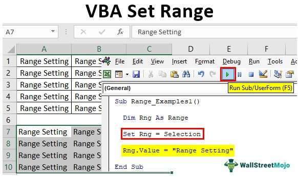
Assume you want whatever the selected cell should be a reference, then we can set the reference as follows.

Code:

Sub Range_Examples()

  Dim Rng As Range

  Set Rng = Selection

  Rng.Value = "Range Setting"

End Sub

This one is a beauty because if we select any of the cells and run it, it will also insert the value to those cells.

For example, we will select certain cells.

Now, we will execute the code and see what happens.

For all the selected cells, it has inserted the value.

Like this, we can set the range reference by declaring variables in VBAVariable declaration is necessary in VBA to define a variable for a specific data type so that it can hold values; any variable that is not defined in VBA cannot hold values.read more.

Things to Remember

The range can select multiple cells, but CELLS can select one cell at a time.
RANGE is an object, and CELLS is property.
Any object variable should be the object’s reference using the SET keyword.

Присвоение диапазона ячеек переменной

Чтобы переменной присвоить диапазон ячеек, она должна быть объявлена как Variant, Object или Range:

Dim myRange1 As Variant

Dim myRange2 As Object

Dim myRange3 As Range

Чтобы было понятнее, для чего переменная создана, объявляйте ее как Range.

Присваивается переменной диапазон ячеек с помощью оператора Set:

Set myRange1 = Range(«B5:E16»)

Set myRange2 = Range(Cells(3, 4), Cells(26, 18))

Set myRange3 = Selection

В выражении Range(Cells(3, 4), Cells(26, 18)) вместо чисел можно использовать переменные.

Для присвоения диапазона ячеек переменной можно использовать встроенное диалоговое окно Application.InputBox, которое позволяет выбрать диапазон на рабочем листе для дальнейшей работы с ним.

Адресация ячеек в диапазоне

К ячейкам присвоенного диапазона можно обращаться по их индексам, а также по индексам строк и столбцов, на пересечении которых они находятся.

Индексация ячеек в присвоенном диапазоне осуществляется слева направо и сверху вниз, например, для диапазона размерностью 5х5:

1	2	3	4	5
6	7	8	9	10
11	12	13	14	15
16	17	18	19	20
21	22	23	24	25

Индексация строк и столбцов начинается с левой верхней ячейки. В диапазоне этого примера содержится 5 строк и 5 столбцов. На пересечении 2 строки и 4 столбца находится ячейка с индексом 9. Обратиться к ней можно так:

‘обращение по индексам строки и столбца

myRange.Cells(2, 4)

‘обращение по индексу ячейки

myRange.Cells(9)

Обращаться в переменной диапазона можно не только к отдельным ячейкам, но и к части диапазона (поддиапазону), присвоенного переменной, например,

обращение к первой строке присвоенного диапазона размерностью 5х5:

myRange.Range(«A1:E1»)

‘или

myRange.Range(Cells(1, 1), Cells(1, 5))

и обращение к первому столбцу присвоенного диапазона размерностью 5х5:

myRange.Range(«A1:A5»)

‘или

myRange.Range(Cells(1, 1), Cells(5, 1))

Работа с диапазоном в переменной

Работать с диапазоном в переменной можно точно также, как и с диапазоном на рабочем листе. Все свойства и методы объекта Range действительны и для диапазона, присвоенного переменной. При обращении к ячейке без указания свойства по умолчанию возвращается ее значение. Строки

MsgBox myRange.Cells(6)

MsgBox myRange.Cells(6).Value

равнозначны. В обоих случаях информационное сообщение MsgBox выведет значение ячейки с индексом 6.

Важно: если вы планируете работать только со значениями, используйте переменные массивов, код в них работает значительно быстрее.

Преимущество работы с диапазоном ячеек в объектной переменной заключается в том, что все изменения, внесенные в переменной, применяются к диапазону (который присвоен переменной) на рабочем листе.

Пример 1 — работа со значениями

Скопируйте процедуру в программный модуль и запустите ее выполнение.

Sub Test1()

‘Объявляем переменную

Dim myRange As Range

‘Присваиваем диапазон ячеек

Set myRange = Range(«C6:E8»)

‘Заполняем первую строку

‘Присваиваем значение первой ячейке

myRange.Cells(1, 1) = 5

‘Присваиваем значение второй ячейке

myRange.Cells(1, 2) = 10

‘Присваиваем третьей ячейке

‘значение выражения

myRange.Cells(1, 3) = myRange.Cells(1, 1) _

* myRange.Cells(1, 2)

‘Заполняем вторую строку

myRange.Cells(2, 1) = 20

myRange.Cells(2, 2) = 25

myRange.Cells(2, 3) = myRange.Cells(2, 1) _

+ myRange.Cells(2, 2)

‘Заполняем третью строку

myRange.Cells(3, 1) = «VBA»

myRange.Cells(3, 2) = «Excel»

myRange.Cells(3, 3) = myRange.Cells(3, 1) _

& » « & myRange.Cells(3, 2)

End Sub

Обратите внимание, что ячейки диапазона на рабочем листе заполнились так же, как и ячейки в переменной диапазона, что доказывает их непосредственную связь между собой.

Пример 2 — работа с форматами

Продолжаем работу с тем же диапазоном рабочего листа «C6:E8»:

Sub Test2()

‘Объявляем переменную

Dim myRange As Range

‘Присваиваем диапазон ячеек

Set myRange = Range(«C6:E8»)

‘Первую строку выделяем жирным шрифтом

myRange.Range(«A1:C1»).Font.Bold = True

‘Вторую строку выделяем фоном

myRange.Range(«A2:C2»).Interior.Color = vbGreen

‘Третьей строке добавляем границы

myRange.Range(«A3:C3»).Borders.LineStyle = True

End Sub

Опять же, обратите внимание, что все изменения форматов в присвоенном диапазоне отобразились на рабочем листе, несмотря на то, что мы непосредственно с ячейками рабочего листа не работали.

Пример 3 — копирование и вставка диапазона из переменной

Значения ячеек диапазона, присвоенного переменной, передаются в другой диапазон рабочего листа с помощью оператора присваивания.

Скопировать и вставить диапазон полностью со значениями и форматами можно при помощи метода Copy, указав место вставки (ячейку) на рабочем листе.

В примере используется тот же диапазон, что и в первых двух, так как он уже заполнен значениями и форматами.

Sub Test3()

‘Объявляем переменную

Dim myRange As Range

‘Присваиваем диапазон ячеек

Set myRange = Range(«C6:E8»)

‘Присваиваем ячейкам рабочего листа

‘значения ячеек переменной диапазона

Range(«A1:C3») = myRange.Value

MsgBox «Пауза»

‘Копирование диапазона переменной

‘и вставка его на рабочий лист

‘с указанием начальной ячейки

myRange.Copy Range(«E1»)

MsgBox «Пауза»

‘Копируем и вставляем часть

‘диапазона из переменной

myRange.Range(«A2:C2»).Copy Range(«E11»)

End Sub

Информационное окно MsgBox добавлено, чтобы вы могли увидеть работу процедуры поэтапно, если решите проверить ее в своей книге Excel.

Размер диапазона в переменной

При получении диапазона с помощью метода Application.InputBox и присвоении его переменной диапазона, бывает полезно узнать его размерность. Это можно сделать следующим образом:

Sub Test4()

‘Объявляем переменную

Dim myRange As Range

‘Присваиваем диапазон ячеек

Set myRange = Application.InputBox(«Выберите диапазон ячеек:», , , , , , , 8)

‘Узнаем количество строк и столбцов

MsgBox «Количество строк = « & myRange.Rows.Count _

& vbNewLine & «Количество столбцов = « & myRange.Columns.Count

End Sub

Запустите процедуру, выберите на рабочем листе Excel любой диапазон и нажмите кнопку «OK». Информационное сообщение выведет количество строк и столбцов в диапазоне, присвоенном переменной myRange.

Источник

На чтение 18 мин. Просмотров 75.1k.

сэр Артур Конан Дойл

Это большая ошибка — теоретизировать, прежде чем кто-то получит данные

Эта статья охватывает все, что вам нужно знать об использовании ячеек и диапазонов в VBA. Вы можете прочитать его от начала до конца, так как он сложен в логическом порядке. Или использовать оглавление ниже, чтобы перейти к разделу по вашему выбору.

Рассматриваемые темы включают свойство смещения, чтение
значений между ячейками, чтение значений в массивы и форматирование ячеек.

Содержание

Краткое руководство по диапазонам и клеткам
Введение
Важное замечание
Свойство Range
Свойство Cells рабочего листа
Использование Cells и Range вместе
Свойство Offset диапазона
Использование диапазона CurrentRegion
Использование Rows и Columns в качестве Ranges
Использование Range вместо Worksheet
Чтение значений из одной ячейки в другую
Использование метода Range.Resize
Чтение Value в переменные
Как копировать и вставлять ячейки
Чтение диапазона ячеек в массив
Пройти через все клетки в диапазоне
Форматирование ячеек
Основные моменты

Краткое руководство по диапазонам и клеткам

Функция	Принимает	Возвращает	Пример	Вид
Range	адреса ячеек	диапазон ячеек	.Range(«A1:A4»)	$A$1:$A$4
Cells	строка, столбец	одна ячейка	.Cells(1,5)	$E$1
Offset	строка, столбец	диапазон	.Range(«A1:A2») .Offset(1,2)	$C$2:$C$3
Rows	строка (-и)	одна или несколько строк	.Rows(4) .Rows(«2:4»)	$4:$4 $2:$4
Columns	столбец (-цы)	один или несколько столбцов	.Columns(4) .Columns(«B:D»)	$D:$D $B:$D

Введение

Это третья статья, посвященная трем основным элементам VBA. Этими тремя элементами являются Workbooks, Worksheets и Ranges/Cells. Cells, безусловно, самая важная часть Excel. Почти все, что вы делаете в Excel, начинается и заканчивается ячейками.

Вы делаете три основных вещи с помощью ячеек:

Читаете из ячейки.
Пишите в ячейку.
Изменяете формат ячейки.

В Excel есть несколько методов для доступа к ячейкам, таких как Range, Cells и Offset. Можно запутаться, так как эти функции делают похожие операции.

В этой статье я расскажу о каждом из них, объясню, почему они вам нужны, и когда вам следует их использовать.

Давайте начнем с самого простого метода доступа к ячейкам — с помощью свойства Range рабочего листа.

Важное замечание

Я недавно обновил эту статью, сейчас использую Value2.

Вам может быть интересно, в чем разница между Value, Value2 и значением по умолчанию:

' Value2
Range("A1").Value2 = 56

' Value
Range("A1").Value = 56

' По умолчанию используется значение
Range("A1") = 56

Использование Value может усечь число, если ячейка отформатирована, как валюта. Если вы не используете какое-либо свойство, по умолчанию используется Value.

Лучше использовать Value2, поскольку он всегда будет возвращать фактическое значение ячейки.

Свойство Range

Рабочий лист имеет свойство Range, которое можно использовать для доступа к ячейкам в VBA. Свойство Range принимает тот же аргумент, что и большинство функций Excel Worksheet, например: «А1», «А3: С6» и т.д.

В следующем примере показано, как поместить значение в ячейку с помощью свойства Range.

Sub ZapisVYacheiku()

    ' Запишите число в ячейку A1 на листе 1 этой книги
    ThisWorkbook.Worksheets("Лист1").Range("A1").Value2 = 67

    ' Напишите текст в ячейку A2 на листе 1 этой рабочей книги
    ThisWorkbook.Worksheets("Лист1").Range("A2").Value2 = "Иван Петров"

    ' Запишите дату в ячейку A3 на листе 1 этой книги
    ThisWorkbook.Worksheets("Лист1").Range("A3").Value2 = #11/21/2019#

End Sub

Как видно из кода, Range является членом Worksheets, которая, в свою очередь, является членом Workbook. Иерархия такая же, как и в Excel, поэтому должно быть легко понять. Чтобы сделать что-то с Range, вы должны сначала указать рабочую книгу и рабочий лист, которому она принадлежит.

В оставшейся части этой статьи я буду использовать кодовое имя для ссылки на лист.

Следующий код показывает приведенный выше пример с использованием кодового имени рабочего листа, т.е. Лист1 вместо ThisWorkbook.Worksheets («Лист1»).

Sub IspKodImya ()

    ' Запишите число в ячейку A1 на листе 1 этой книги    
     Sheet1.Range("A1").Value2 = 67

    ' Напишите текст в ячейку A2 на листе 1 этой рабочей книги
    Sheet1.Range("A2").Value2 = "Иван Петров"

    ' Запишите дату в ячейку A3 на листе 1 этой книги
    Sheet1.Range("A3").Value2 = #11/21/2019#

End Sub

Вы также можете писать в несколько ячеек, используя свойство
Range

Sub ZapisNeskol()

    ' Запишите число в диапазон ячеек
    Sheet1.Range("A1:A10").Value2 = 67

    ' Написать текст в несколько диапазонов ячеек
    Sheet1.Range("B2:B5,B7:B9").Value2 = "Иван Петров"

End Sub

Свойство Cells рабочего листа

У Объекта листа есть другое свойство, называемое Cells, которое очень похоже на Range . Есть два отличия:

Cells возвращают диапазон только одной ячейки.
Cells принимает строку и столбец в качестве аргументов.

В приведенном ниже примере показано, как записывать значения
в ячейки, используя свойства Range и Cells.

Sub IspCells()

    ' Написать в А1
    Sheet1.Range("A1").Value2 = 10
    Sheet1.Cells(1, 1).Value2  = 10

    ' Написать в А10
    Sheet1.Range("A10").Value2 = 10
    Sheet1.Cells(10, 1).Value2  = 10

    ' Написать в E1
    Sheet1.Range("E1").Value2 = 10
    Sheet1.Cells(1, 5).Value2  = 10

End Sub

Вам должно быть интересно, когда использовать Cells, а когда Range. Использование Range полезно для доступа к одним и тем же ячейкам при каждом запуске макроса.

Например, если вы использовали макрос для вычисления суммы и
каждый раз записывали ее в ячейку A10, тогда Range подойдет для этой задачи.

Использование свойства Cells полезно, если вы обращаетесь к
ячейке по номеру, который может отличаться. Проще объяснить это на примере.

В следующем коде мы просим пользователя указать номер столбца. Использование Cells дает нам возможность использовать переменное число для столбца.

Sub ZapisVPervuyuPustuyuYacheiku()

    Dim UserCol As Integer
    
    ' Получить номер столбца от пользователя
    UserCol = Application.InputBox("Пожалуйста, введите номер столбца...", Type:=1)
    
    ' Написать текст в выбранный пользователем столбец
    Sheet1.Cells(1, UserCol).Value2 = "Иван Петров"

End Sub

В приведенном выше примере мы используем номер для столбца,
а не букву.

Чтобы использовать Range здесь, потребуется преобразовать эти значения в ссылку на
буквенно-цифровую ячейку, например, «С1». Использование свойства Cells позволяет нам
предоставить строку и номер столбца для доступа к ячейке.

Иногда вам может понадобиться вернуть более одной ячейки, используя номера строк и столбцов. В следующем разделе показано, как это сделать.

Использование Cells и Range вместе

Как вы уже видели, вы можете получить доступ только к одной ячейке, используя свойство Cells. Если вы хотите вернуть диапазон ячеек, вы можете использовать Cells с Range следующим образом:

Sub IspCellsSRange()

    With Sheet1
        ' Запишите 5 в диапазон A1: A10, используя свойство Cells
        .Range(.Cells(1, 1), .Cells(10, 1)).Value2 = 5

        ' Диапазон B1: Z1 будет выделен жирным шрифтом
        .Range(.Cells(1, 2), .Cells(1, 26)).Font.Bold = True

    End With

End Sub

Как видите, вы предоставляете начальную и конечную ячейку
диапазона. Иногда бывает сложно увидеть, с каким диапазоном вы имеете дело,
когда значением являются все числа. Range имеет свойство Address, которое
отображает буквенно-цифровую ячейку для любого диапазона. Это может
пригодиться, когда вы впервые отлаживаете или пишете код.

В следующем примере мы распечатываем адрес используемых нами
диапазонов.

Sub PokazatAdresDiapazona()

    ' Примечание. Использование подчеркивания позволяет разделить строки кода.
    With Sheet1

        ' Запишите 5 в диапазон A1: A10, используя свойство Cells
        .Range(.Cells(1, 1), .Cells(10, 1)).Value2 = 5
        Debug.Print "Первый адрес: " _
            + .Range(.Cells(1, 1), .Cells(10, 1)).Address

        ' Диапазон B1: Z1 будет выделен жирным шрифтом
        .Range(.Cells(1, 2), .Cells(1, 26)).Font.Bold = True
        Debug.Print "Второй адрес : " _
            + .Range(.Cells(1, 2), .Cells(1, 26)).Address

    End With

End Sub

В примере я использовал Debug.Print для печати в Immediate Window. Для просмотра этого окна выберите «View» -> «в Immediate Window» (Ctrl + G).

Свойство Offset диапазона

У диапазона есть свойство, которое называется Offset. Термин «Offset» относится к отсчету от исходной позиции. Он часто используется в определенных областях программирования. С помощью свойства «Offset» вы можете получить диапазон ячеек того же размера и на определенном расстоянии от текущего диапазона. Это полезно, потому что иногда вы можете выбрать диапазон на основе определенного условия. Например, на скриншоте ниже есть столбец для каждого дня недели. Учитывая номер дня (т.е. понедельник = 1, вторник = 2 и т.д.). Нам нужно записать значение в правильный столбец.

Сначала мы попытаемся сделать это без использования Offset.

' Это Sub тесты с разными значениями
Sub TestSelect()

    ' Понедельник
    SetValueSelect 1, 111.21
    ' Среда
    SetValueSelect 3, 456.99
    ' Пятница
    SetValueSelect 5, 432.25
    ' Воскресение
    SetValueSelect 7, 710.17

End Sub

' Записывает значение в столбец на основе дня
Public Sub SetValueSelect(lDay As Long, lValue As Currency)

    Select Case lDay
        Case 1: Sheet1.Range("H3").Value2 = lValue
        Case 2: Sheet1.Range("I3").Value2 = lValue
        Case 3: Sheet1.Range("J3").Value2 = lValue
        Case 4: Sheet1.Range("K3").Value2 = lValue
        Case 5: Sheet1.Range("L3").Value2 = lValue
        Case 6: Sheet1.Range("M3").Value2 = lValue
        Case 7: Sheet1.Range("N3").Value2 = lValue
    End Select

End Sub

Как видно из примера, нам нужно добавить строку для каждого возможного варианта. Это не идеальная ситуация. Использование свойства Offset обеспечивает более чистое решение.

' Это Sub тесты с разными значениями
Sub TestOffset()

    DayOffSet 1, 111.01
    DayOffSet 3, 456.99
    DayOffSet 5, 432.25
    DayOffSet 7, 710.17

End Sub

Public Sub DayOffSet(lDay As Long, lValue As Currency)

    ' Мы используем значение дня с Offset, чтобы указать правильный столбец
    Sheet1.Range("G3").Offset(, lDay).Value2 = lValue

End Sub

Как видите, это решение намного лучше. Если количество дней увеличилось, нам больше не нужно добавлять код. Чтобы Offset был полезен, должна быть какая-то связь между позициями ячеек. Если столбцы Day в приведенном выше примере были случайными, мы не могли бы использовать Offset. Мы должны были бы использовать первое решение.

Следует иметь в виду, что Offset сохраняет размер диапазона. Итак .Range («A1:A3»).Offset (1,1) возвращает диапазон B2:B4. Ниже приведены еще несколько примеров использования Offset.

Sub IspOffset()

    ' Запись в В2 - без Offset
    Sheet1.Range("B2").Offset().Value2 = "Ячейка B2"

    ' Написать в C2 - 1 столбец справа
    Sheet1.Range("B2").Offset(, 1).Value2 = "Ячейка C2"

    ' Написать в B3 - 1 строка вниз
    Sheet1.Range("B2").Offset(1).Value2 = "Ячейка B3"

    ' Запись в C3 - 1 столбец справа и 1 строка вниз
    Sheet1.Range("B2").Offset(1, 1).Value2 = "Ячейка C3"

    ' Написать в A1 - 1 столбец слева и 1 строка вверх
    Sheet1.Range("B2").Offset(-1, -1).Value2 = "Ячейка A1"

    ' Запись в диапазон E3: G13 - 1 столбец справа и 1 строка вниз
    Sheet1.Range("D2:F12").Offset(1, 1).Value2 = "Ячейки E3:G13"

End Sub

Использование диапазона CurrentRegion

CurrentRegion возвращает диапазон всех соседних ячеек в данный диапазон. На скриншоте ниже вы можете увидеть два CurrentRegion. Я добавил границы, чтобы прояснить CurrentRegion.

Строка или столбец пустых ячеек означает конец CurrentRegion.

Вы можете вручную проверить
CurrentRegion в Excel, выбрав диапазон и нажав Ctrl + Shift + *.

Если мы возьмем любой диапазон
ячеек в пределах границы и применим CurrentRegion, мы вернем диапазон ячеек во
всей области.

Например:

Range («B3»). CurrentRegion вернет диапазон B3:D14

Range («D14»). CurrentRegion вернет диапазон B3:D14

Range («C8:C9»). CurrentRegion вернет диапазон B3:D14 и так далее

Как пользоваться

Мы получаем CurrentRegion следующим образом

' CurrentRegion вернет B3:D14 из приведенного выше примера
Dim rg As Range
Set rg = Sheet1.Range("B3").CurrentRegion

Только чтение строк данных

Прочитать диапазон из второй строки, т.е. пропустить строку заголовка.

' CurrentRegion вернет B3:D14 из приведенного выше примера
Dim rg As Range
Set rg = Sheet1.Range("B3").CurrentRegion

' Начало в строке 2 - строка после заголовка
Dim i As Long
For i = 2 To rg.Rows.Count
    ' текущая строка, столбец 1 диапазона
    Debug.Print rg.Cells(i, 1).Value2
Next i

Удалить заголовок

Удалить строку заголовка (т.е. первую строку) из диапазона. Например, если диапазон — A1:D4, это возвратит A2:D4

' CurrentRegion вернет B3:D14 из приведенного выше примера
Dim rg As Range
Set rg = Sheet1.Range("B3").CurrentRegion

' Удалить заголовок
Set rg = rg.Resize(rg.Rows.Count - 1).Offset(1)

' Начните со строки 1, так как нет строки заголовка
Dim i As Long
For i = 1 To rg.Rows.Count
    ' текущая строка, столбец 1 диапазона
    Debug.Print rg.Cells(i, 1).Value2
Next i

Использование Rows и Columns в качестве Ranges

Если вы хотите что-то сделать со всей строкой или столбцом,
вы можете использовать свойство «Rows и
Columns» на рабочем листе. Они оба принимают один параметр — номер строки
или столбца, к которому вы хотите получить доступ.

Sub IspRowIColumns()

    ' Установите размер шрифта столбца B на 9
    Sheet1.Columns(2).Font.Size = 9

    ' Установите ширину столбцов от D до F
    Sheet1.Columns("D:F").ColumnWidth = 4

    ' Установите размер шрифта строки 5 до 18
    Sheet1.Rows(5).Font.Size = 18

End Sub

Использование Range вместо Worksheet

Вы также можете использовать Cella, Rows и Columns, как часть Range, а не как часть Worksheet. У вас может быть особая необходимость в этом, но в противном случае я бы избегал практики. Это делает код более сложным. Простой код — твой друг. Это уменьшает вероятность ошибок.

Код ниже выделит второй столбец диапазона полужирным. Поскольку диапазон имеет только две строки, весь столбец считается B1:B2

Sub IspColumnsVRange()

    ' Это выделит B1 и B2 жирным шрифтом.
    Sheet1.Range("A1:C2").Columns(2).Font.Bold = True

End Sub

Чтение значений из одной ячейки в другую

В большинстве примеров мы записали значения в ячейку. Мы
делаем это, помещая диапазон слева от знака равенства и значение для размещения
в ячейке справа. Для записи данных из одной ячейки в другую мы делаем то же
самое. Диапазон назначения идет слева, а диапазон источника — справа.

В следующем примере показано, как это сделать:

Sub ChitatZnacheniya()

    ' Поместите значение из B1 в A1
    Sheet1.Range("A1").Value2 = Sheet1.Range("B1").Value2

    ' Поместите значение из B3 в лист2 в ячейку A1
    Sheet1.Range("A1").Value2 = Sheet2.Range("B3").Value2

    ' Поместите значение от B1 в ячейки A1 до A5
    Sheet1.Range("A1:A5").Value2 = Sheet1.Range("B1").Value2

    ' Вам необходимо использовать свойство «Value», чтобы прочитать несколько ячеек
    Sheet1.Range("A1:A5").Value2 = Sheet1.Range("B1:B5").Value2

End Sub

Как видно из этого примера, невозможно читать из нескольких ячеек. Если вы хотите сделать это, вы можете использовать функцию копирования Range с параметром Destination.

Sub KopirovatZnacheniya()

    ' Сохранить диапазон копирования в переменной
    Dim rgCopy As Range
    Set rgCopy = Sheet1.Range("B1:B5")

    ' Используйте это для копирования из более чем одной ячейки
    rgCopy.Copy Destination:=Sheet1.Range("A1:A5")

    ' Вы можете вставить в несколько мест назначения
    rgCopy.Copy Destination:=Sheet1.Range("A1:A5,C2:C6")

End Sub

Функция Copy копирует все, включая формат ячеек. Это тот же результат, что и ручное копирование и вставка выделения. Подробнее об этом вы можете узнать в разделе «Копирование и вставка ячеек»

Использование метода Range.Resize

При копировании из одного диапазона в другой с использованием присваивания (т.е. знака равенства) диапазон назначения должен быть того же размера, что и исходный диапазон.

Использование функции Resize позволяет изменить размер
диапазона до заданного количества строк и столбцов.

Например:

Sub ResizePrimeri()
 
    ' Печатает А1
    Debug.Print Sheet1.Range("A1").Address

    ' Печатает A1:A2
    Debug.Print Sheet1.Range("A1").Resize(2, 1).Address

    ' Печатает A1:A5
    Debug.Print Sheet1.Range("A1").Resize(5, 1).Address
    
    ' Печатает A1:D1
    Debug.Print Sheet1.Range("A1").Resize(1, 4).Address
    
    ' Печатает A1:C3
    Debug.Print Sheet1.Range("A1").Resize(3, 3).Address
    
End Sub

Когда мы хотим изменить наш целевой диапазон, мы можем
просто использовать исходный размер диапазона.

Другими словами, мы используем количество строк и столбцов
исходного диапазона в качестве параметров для изменения размера:

Sub Resize()

    Dim rgSrc As Range, rgDest As Range
    
    ' Получить все данные в текущей области
    Set rgSrc = Sheet1.Range("A1").CurrentRegion

      ' Получить диапазон назначения
    Set rgDest = Sheet2.Range("A1")
    Set rgDest = rgDest.Resize(rgSrc.Rows.Count, rgSrc.Columns.Count)
    
    rgDest.Value2 = rgSrc.Value2

End Sub

Мы можем сделать изменение размера в одну строку, если нужно:

Sub Resize2()

    Dim rgSrc As Range
    
    ' Получить все данные в ткущей области
    Set rgSrc = Sheet1.Range("A1").CurrentRegion
    
    With rgSrc
        Sheet2.Range("A1").Resize(.Rows.Count, .Columns.Count) = .Value2
    End With
    
End Sub

Чтение Value в переменные

Мы рассмотрели, как читать из одной клетки в другую. Вы также можете читать из ячейки в переменную. Переменная используется для хранения значений во время работы макроса. Обычно вы делаете это, когда хотите манипулировать данными перед тем, как их записать. Ниже приведен простой пример использования переменной. Как видите, значение элемента справа от равенства записывается в элементе слева от равенства.

Sub IspVar()

    ' Создайте
    Dim val As Integer

    ' Читать число из ячейки
    val = Sheet1.Range("A1").Value2

    ' Добавить 1 к значению
    val = val + 1

    ' Запишите новое значение в ячейку
    Sheet1.Range("A2").Value2 = val

End Sub

Для чтения текста в переменную вы используете переменную
типа String.

Sub IspVarText()

    ' Объявите переменную типа string
    Dim sText As String

    ' Считать значение из ячейки
    sText = Sheet1.Range("A1").Value2

    ' Записать значение в ячейку
    Sheet1.Range("A2").Value2 = sText

End Sub

Вы можете записать переменную в диапазон ячеек. Вы просто
указываете диапазон слева, и значение будет записано во все ячейки диапазона.

Sub VarNeskol()

    ' Считать значение из ячейки
    Sheet1.Range("A1:B10").Value2 = 66

End Sub

Вы не можете читать из нескольких ячеек в переменную. Однако
вы можете читать массив, который представляет собой набор переменных. Мы
рассмотрим это в следующем разделе.

Как копировать и вставлять ячейки

Если вы хотите скопировать и вставить диапазон ячеек, вам не
нужно выбирать их. Это распространенная ошибка, допущенная новыми пользователями
VBA.

Вы можете просто скопировать ряд ячеек, как здесь:

Range("A1:B4").Copy Destination:=Range("C5")

При использовании этого метода копируется все — значения,
форматы, формулы и так далее. Если вы хотите скопировать отдельные элементы, вы
можете использовать свойство PasteSpecial
диапазона.

Работает так:

Range("A1:B4").Copy
Range("F3").PasteSpecial Paste:=xlPasteValues
Range("F3").PasteSpecial Paste:=xlPasteFormats
Range("F3").PasteSpecial Paste:=xlPasteFormulas

В следующей таблице приведен полный список всех типов вставок.

Виды вставок

xlPasteAll

xlPasteAllExceptBorders

xlPasteAllMergingConditionalFormats

xlPasteAllUsingSourceTheme

xlPasteColumnWidths

xlPasteComments

xlPasteFormats

xlPasteFormulas

xlPasteFormulasAndNumberFormats

xlPasteValidation

xlPasteValues

xlPasteValuesAndNumberFormats

Чтение диапазона ячеек в массив

Вы также можете скопировать значения, присвоив значение
одного диапазона другому.

Range("A3:Z3").Value2 = Range("A1:Z1").Value2

Значение диапазона в этом примере считается вариантом массива. Это означает, что вы можете легко читать из диапазона ячеек в массив. Вы также можете писать из массива в диапазон ячеек. Если вы не знакомы с массивами, вы можете проверить их в этой статье.

В следующем коде показан пример использования массива с
диапазоном.

Sub ChitatMassiv()

    ' Создать динамический массив
    Dim StudentMarks() As Variant

    ' Считать 26 значений в массив из первой строки
    StudentMarks = Range("A1:Z1").Value2

    ' Сделайте что-нибудь с массивом здесь

    ' Запишите 26 значений в третью строку
    Range("A3:Z3").Value2 = StudentMarks

End Sub

Имейте в виду, что массив, созданный для чтения, является
двумерным массивом. Это связано с тем, что электронная таблица хранит значения
в двух измерениях, то есть в строках и столбцах.

Пройти через все клетки в диапазоне

Иногда вам нужно просмотреть каждую ячейку, чтобы проверить значение.

Вы можете сделать это, используя цикл For Each, показанный в следующем коде.

Sub PeremeschatsyaPoYacheikam()

    ' Пройдите через каждую ячейку в диапазоне
    Dim rg As Range
    For Each rg In Sheet1.Range("A1:A10,A20")
        ' Распечатать адрес ячеек, которые являются отрицательными
        If rg.Value < 0 Then
            Debug.Print rg.Address + " Отрицательно."
        End If
    Next

End Sub

Вы также можете проходить последовательные ячейки, используя
свойство Cells и стандартный цикл For.

Стандартный цикл более гибок в отношении используемого вами
порядка, но он медленнее, чем цикл For Each.

Sub PerehodPoYacheikam()
 
    ' Пройдите клетки от А1 до А10
    Dim i As Long
    For i = 1 To 10
        ' Распечатать адрес ячеек, которые являются отрицательными
        If Range("A" & i).Value < 0 Then
            Debug.Print Range("A" & i).Address + " Отрицательно."
        End If
    Next
 
    ' Пройдите в обратном порядке, то есть от A10 до A1
    For i = 10 To 1 Step -1
        ' Распечатать адрес ячеек, которые являются отрицательными
        If Range("A" & i) < 0 Then
            Debug.Print Range("A" & i).Address + " Отрицательно."
        End If
    Next
 
End Sub

Форматирование ячеек

Иногда вам нужно будет отформатировать ячейки в электронной
таблице. Это на самом деле очень просто. В следующем примере показаны различные
форматы, которые можно добавить в любой диапазон ячеек.

Sub FormatirovanieYacheek()

    With Sheet1

        ' Форматировать шрифт
        .Range("A1").Font.Bold = True
        .Range("A1").Font.Underline = True
        .Range("A1").Font.Color = rgbNavy

        ' Установите числовой формат до 2 десятичных знаков
        .Range("B2").NumberFormat = "0.00"
        ' Установите числовой формат даты
        .Range("C2").NumberFormat = "dd/mm/yyyy"
        ' Установите формат чисел на общий
        .Range("C3").NumberFormat = "Общий"
        ' Установить числовой формат текста
        .Range("C4").NumberFormat = "Текст"

        ' Установите цвет заливки ячейки
        .Range("B3").Interior.Color = rgbSandyBrown

        ' Форматировать границы
        .Range("B4").Borders.LineStyle = xlDash
        .Range("B4").Borders.Color = rgbBlueViolet

    End With

End Sub

Основные моменты

Ниже приводится краткое изложение основных моментов

Range возвращает диапазон ячеек
Cells возвращают только одну клетку
Вы можете читать из одной ячейки в другую
Вы можете читать из диапазона ячеек в другой диапазон ячеек.
Вы можете читать значения из ячеек в переменные и наоборот.
Вы можете читать значения из диапазонов в массивы и наоборот
Вы можете использовать цикл For Each или For, чтобы проходить через каждую ячейку в диапазоне.
Свойства Rows и Columns позволяют вам получить доступ к диапазону ячеек этих типов

Источник

What’s in the name?

If you are working with Excel spreadsheets, it could mean a lot of time saving and efficiency.

In this tutorial, you’ll learn how to create Named Ranges in Excel and how to use it to save time.

Named Ranges in Excel – An Introduction
Benefits of Creating Named Ranges in Excel
- Use Names instead of Cell References
- No Need to Go Back to the Dataset to Select Cells
- Named Ranges Make Formulas Dynamic
How to Create Named Ranges in Excel
- Method #1 – Using Define Name
- Method #2: Using the Name Box
- Method #3: Using Create From Selection Option
- Naming Convention for Named Ranges in Excel
Too Many Named Ranges in Excel? Don’t Worry
- Getting the Names of All the Named Ranges
- Displaying the Matching Named Ranges
How to Edit Named Ranges in Excel
Useful Named Range Shortcuts (the Power of F3)
Creating Dynamic Named Ranges in Excel
- How does Dynamic Named Ranges Work?

Named Ranges in Excel – An Introduction

If someone has to call me or refer to me, they will use my name (instead of saying a male is staying in so and so place with so and so height and weight).

Right?

Similarly, in Excel, you can give a name to a cell or a range of cells.

Now, instead of using the cell reference (such as A1 or A1:A10), you can simply use the name that you assigned to it.

For example, suppose you have a data set as shown below:

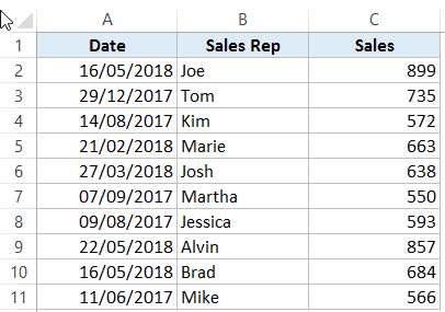
In this data set, if you have to refer to the range that has the Date, you will have to use A2:A11 in formulas. Similarly, for Sales Rep and Sales, you will have to use B2:B11 and C2:C11.

While it’s alright when you only have a couple of data points, but in case you huge complex data sets, using cell references to refer to data could be time-consuming.

Excel Named Ranges makes it easy to refer to data sets in Excel.

You can create a named range in Excel for each data category, and then use that name instead of the cell references. For example, dates can be named ‘Date’, Sales Rep data can be named ‘SalesRep’ and sales data can be named ‘Sales’.

You can also create a name for a single cell. For example, if you have the sales commission percentage in a cell, you can name that cell as ‘Commission’.

Benefits of Creating Named Ranges in Excel

Here are the benefits of using named ranges in Excel.

Use Names instead of Cell References

When you create Named Ranges in Excel, you can use these names instead of the cell references.

For example, you can use =SUM(SALES) instead of =SUM(C2:C11) for the above data set.

Have a look at ṭhe formulas listed below. Instead of using cell references, I have used the Named Ranges.

Number of sales with value more than 500: =COUNTIF(Sales,”>500″)
Sum of all the sales done by Tom: =SUMIF(SalesRep,”Tom”,Sales)
Commission earned by Joe (sales by Joe multiplied by commission percentage):
=SUMIF(SalesRep,”Joe”,Sales)*Commission

You would agree that these formulas are easy to create and easy to understand (especially when you share it with someone else or revisit it yourself.

No Need to Go Back to the Dataset to Select Cells

Another significant benefit of using Named Ranges in Excel is that you don’t need to go back and select the cell ranges.

You can just type a couple of alphabets of that named range and Excel will show the matching named ranges (as shown below):

Named Ranges Make Formulas Dynamic

By using Named Ranges in Excel, you can make Excel formulas dynamic.

For example, in the case of sales commission, instead of using the value 2.5%, you can use the Named Range.

Now, if your company later decides to increase the commission to 3%, you can simply update the Named Range, and all the calculation would automatically update to reflect the new commission.

How to Create Named Ranges in Excel

Here are three ways to create Named Ranges in Excel:

Method #1 – Using Define Name

Here are the steps to create Named Ranges in Excel using Define Name:

This will create a Named Range SALESREP.

Method #2: Using the Name Box

Select the range for which you want to create a name (do not select headers).
Go to the Name Box on the left of Formula bar and Type the name of the with which you want to create the Named Range.
Note that the Name created here will be available for the entire Workbook. If you wish to restrict it to a worksheet, use Method 1.

Method #3: Using Create From Selection Option

This is the recommended way when you have data in tabular form, and you want to create named range for each column/row.

For example, in the dataset below, if you want to quickly create three named ranges (Date, Sales_Rep, and Sales), then you can use the method shown below.

Here are the steps to quickly create named ranges from a dataset:

This will create three Named Ranges – Date, Sales_Rep, and Sales.

Note that it automatically picks up names from the headers. If there are any space between words, it inserts an underscore (as you can’t have spaces in named ranges).

Naming Convention for Named Ranges in Excel

There are certain naming rules you need to know while creating Named Ranges in Excel:

The first character of a Named Range should be a letter and underscore character(_), or a backslash(). If it’s anything else, it will show an error. The remaining characters can be letters, numbers, special characters, period, or underscore.
You can not use names that also represent cell references in Excel. For example, you can’t use AB1 as it is also a cell reference.
You can’t use spaces while creating named ranges. For example, you can’t have Sales Rep as a named range. If you want to combine two words and create a Named Range, use an underscore, period or uppercase characters to create it. For example, you can have Sales_Rep, SalesRep, or SalesRep.
- While creating named ranges, Excel treats uppercase and lowercase the same way. For example, if you create a named range SALES, then you will not be able to create another named range such as ‘sales’ or ‘Sales’.
A Named Range can be up to 255 characters long.

Too Many Named Ranges in Excel? Don’t Worry

Sometimes in large data sets and complex models, you may end up creating a lot of Named Ranges in Excel.

What if you don’t remember the name of the Named Range you created?

Don’t worry – here are some useful tips.

Getting the Names of All the Named Ranges

Here are the steps to get a list of all the named ranges you created:

This will give you a list of all the Named Ranges in that workbook. To use a named range (in formulas or a cell), double click on it.

Displaying the Matching Named Ranges

If you have some idea about the Name, type a few initial characters, and Excel will show a drop down of the matching names.

How to Edit Named Ranges in Excel

If you have already created a Named Range, you can edit it using the following steps:

Useful Named Range Shortcuts (the Power of F3)

Here are some useful keyboard shortcuts that will come handy when you are working with Named Ranges in Excel:

To get a list of all the Named Ranges and pasting it in Formula: F3
To create new name using Name Manager Dialogue Box: Control + F3
To create Named Ranges from Selection: Control + Shift + F3

Creating Dynamic Named Ranges in Excel

So far in this tutorial, we have created static Named Ranges.

This means that these Named Ranges would always refer to the same dataset.

For example, if A1:A10 has been named as ‘Sales’, it would always refer to A1:A10.

If you add more sales data, then you would have to manually go and update the reference in the named range.

In the world of ever-expanding data sets, this may end up taking up a lot of your time. Every time you get new data, you may have to update the Named Ranges in Excel.

To tackle this issue, we can create Dynamic Named Ranges in Excel that would automatically account for additional data and include it in the existing Named Range.

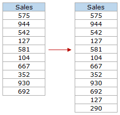
For example, For example, if I add two additional sales data points, a dynamic named range would automatically refer to A1:A12.

This kind of Dynamic Named Range can be created by using Excel INDEX function. Instead of specifying the cell references while creating the Named Range, we specify the formula. The formula automatically updated when the data is added or deleted.

Let’s see how to create Dynamic Named Ranges in Excel.

Suppose we have the sales data in cell A2:A11.

Here are the steps to create Dynamic Named Ranges in Excel:

1. Go to the Formula tab and click on Define Name.
2. In the New Name dialogue box type the following:
  - Name: Sales
  - Scope: Workbook
  - Refers to: =$A$2:INDEX($A$2:$A$100,COUNTIF($A$2:$A$100,”<>”&””))
3. Click OK.

Done!

You now have a dynamic named range with the name ‘Sales’. This would automatically update whenever you add data to it or remove data from it.

How does Dynamic Named Ranges Work?

To explain how this work, you need to know a bit more about Excel INDEX function.

Most people use INDEX to return a value from a list based on the row and column number.

But the INDEX function also has another side to it.

It can be used to return a cell reference when it is used as a part of a cell reference.

For example, here is the formula that we have used to create a dynamic named range:

=$A$2:INDEX($A$2:$A$100,COUNTIF($A$2:$A$100,"<>"&""))

INDEX($A$2:$A$100,COUNTIF($A$2:$A$100,”<>”&””) –> This part of the formula is expected to return a value (which would be the 10th value from the list, considering there are ten items).

However, when used in front of a reference (=$A$2:INDEX($A$2:$A$100,COUNTIF($A$2:$A$100,”<>”&””))) it returns the reference to the cell instead of the value.

Hence, here it returns =$A$2:$A$11

If we add two additional values to the sales column, it would then return =$A$2:$A$13

When you add new data to the list, Excel COUNTIF function returns the number of non-blank cells in the data. This number is used by the INDEX function to fetch the cell reference of the last item in the list.

Note:

This would only work if there are no blank cells in the data.
In the example taken above, I have assigned a large number of cells (A2:A100) for the Named Range formula. You can adjust this based on your data set.

You can also use OFFSET function to create a Dynamic Named Ranges in Excel, however, since OFFSET function is volatile, it may lead a slow Excel workbook. INDEX, on the other hand, is semi-volatile, which makes it a better choice to create Dynamic Named Ranges in Excel.

You may also like the following Excel resources:

Free Excel Templates.
Free Online Excel Training (7-Part Online Video Course).
Useful Excel Macro Code Examples.
10 Advanced Excel VLOOKUP Examples.
Creating a Drop Down List in Excel.
Creating a Named Range in Google Sheets.
How to Reference Another Sheet or Workbook in Excel
How to Delete Named Range in Excel?

Источник

Excel VBA Set Range

How to Use Set Range in VBA Excel?

Example #1

Example #2

Example #3

Pros of VBA Set Range

Things to Remember

Recommended Articles

Set Range in Excel VBA

Table of contents

How to Access the Range of Cells in Excel VBA?

Accessing Multiple Cells & Setting Range Reference in VBA

Things to Remember

Recommended Articles

Присвоение диапазона ячеек переменной

Адресация ячеек в диапазоне

Работа с диапазоном в переменной

Пример 1 — работа со значениями

Пример 2 — работа с форматами

Пример 3 — копирование и вставка диапазона из переменной

Размер диапазона в переменной

Краткое руководство по диапазонам и клеткам

Введение

Важное замечание

Свойство Range

Свойство Cells рабочего листа

Использование Cells и Range вместе

Свойство Offset диапазона

Использование диапазона CurrentRegion

Использование Rows и Columns в качестве Ranges

Использование Range вместо Worksheet

Чтение значений из одной ячейки в другую

Использование метода Range.Resize

Чтение Value в переменные

Как копировать и вставлять ячейки

Чтение диапазона ячеек в массив

Пройти через все клетки в диапазоне

Форматирование ячеек

Основные моменты

Named Ranges in Excel – An Introduction

Benefits of Creating Named Ranges in Excel

Use Names instead of Cell References

No Need to Go Back to the Dataset to Select Cells

Named Ranges Make Formulas Dynamic

How to Create Named Ranges in Excel

Method #1 – Using Define Name

Method #2: Using the Name Box

Method #3: Using Create From Selection Option

Naming Convention for Named Ranges in Excel

Too Many Named Ranges in Excel? Don’t Worry

Getting the Names of All the Named Ranges

Displaying the Matching Named Ranges

How to Edit Named Ranges in Excel

Useful Named Range Shortcuts (the Power of F3)

Creating Dynamic Named Ranges in Excel

How does Dynamic Named Ranges Work?