
Bottom line: Learn how to create macros that apply filters to ranges and Tables with the AutoFilter method in VBA. The post contains links to examples for filtering different data types including text, numbers, dates, colors, and icons.
Skill level: Intermediate
Download the File
The Excel file that contains the code can be downloaded below. This file contains code for filtering different data types and filter types.
Writing Macros for Filters in Excel
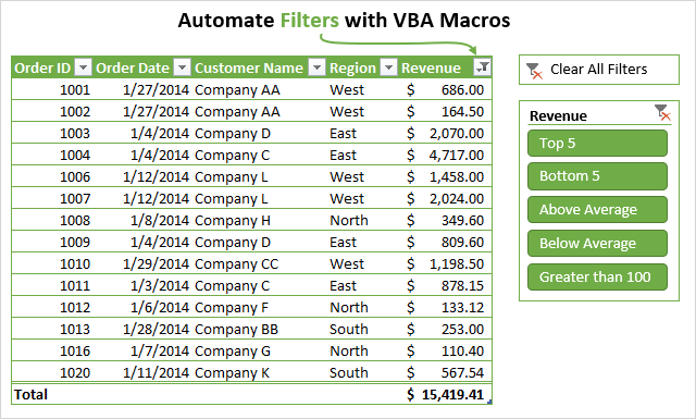
Filters are a great tool for analyzing data in Excel. For most analysts and frequent Excel users, filters are a part of our daily lives. We use the filter drop-down menus to apply filters to individual columns in a data set. This helps us tie out numbers with reports and do investigative work on our data.
Filtering can also be a time consuming process. Especially when we are applying filters to multiple columns on large worksheets, or filtering data to then copy/paste it to other worksheets or workbooks.
This article explains how to create macros to automate the filtering process. This is an extensive guide on the AutoFilter method in VBA.
I also have articles with examples for different filters and data types including: blanks, text, numbers, dates, colors & icons, and clearing filters.
The Macro Recorder is Your Friend (& Enemy)
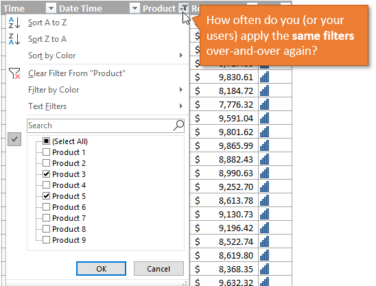
We can easily get the VBA code for filters by turning on the macro recorder, then applying one or more filters to a range/Table.
Here are the steps to create a filter macro with the macro recorder:
- Turn the macro recorder on:
- Developer tab > Record Macro.
- Give the macro a name, choose where you want the code saved, and press OK.
- Apply one or more filters using the filter drop-down menus.
- Stop the recorder.
- Open the VB Editor (Developer tab > Visual Basic) to view the code.
If you’ve already used the macro recorder for this process, then you know how useful it can be. Especially as our filter criteria gets more complex.
The code will look something like the following.
Sub Filters_Macro_Recorder()
'
' Filters_Macro_Recorder Macro
'

'
    ActiveSheet.ListObjects("tblData").Range.AutoFilter Field:=4, Criteria1:= _
        "Product 2"
    ActiveSheet.ListObjects("tblData").Range.AutoFilter Field:=4
    ActiveSheet.ListObjects("tblData").Range.AutoFilter Field:=5, Criteria1:= _
        ">=500", Operator:=xlAnd, Criteria2:="<=1000"
End Sub
We can see that each line uses the AutoFilter method to apply the filter to the column. It also contains information about the criteria for the filter.
This is where it can get complex, confusing, and frustrating. It can be difficult to understand what the code means when trying to modify it for a different data set or scenario. So let’s take a look at how the AutoFilter method works.
The AutoFilter Method Explained
The AutoFilter method is used to clear and apply filters to a single column in a range or Table in VBA. It automates the process of applying filters through the filter drop-down menus, and does all that work for us. 🙂
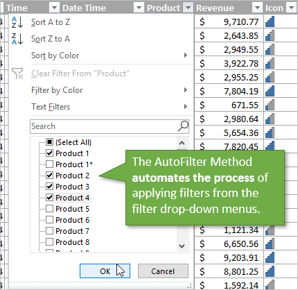
It can be used to apply filters to multiple columns by writing multiple lines of code, one for each column. We can also use AutoFilter to apply multiple filter criteria to a single column, just like you would in the filter drop-down menu by selecting multiple check boxes or specifying a date range.
Writing AutoFilter Code
Here are step-by-step instructions for writing a line of code for AutoFilter
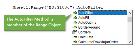
Step 1 : Referencing the Range or Table
The AutoFilter method is a member of the Range object. So we must reference a range or Table that the filters are applied to on the sheet. This will be the entire range that the filters are applied to.
The following examples will enable/disable filters on range B3:G1000 on the AutoFilter Guide sheet.
Sub AutoFilter_Range()
'AutoFilter is a member of the Range object

  'Reference the entire range that the filters are applied to
  'AutoFilter turns filters on/off when no parameters are specified.
  Sheet1.Range("B3:G1000").AutoFilter

  'Fully qualified reference starting at Workbook level
  ThisWorkbook.Worksheets("AutoFilter Guide").Range("B3:G1000").AutoFilter

End Sub
Here is an example using Excel Tables.
Sub AutoFilter_Table()
'AutoFilters on Tables work the same way.

Dim lo As ListObject 'Excel Table

  'Set the ListObject (Table) variable
  Set lo = Sheet1.ListObjects(1)

  'AutoFilter is member of Range object
  'The parent of the Range object is the List Object
  lo.Range.AutoFilter

End Sub
The AutoFilter method has 5 optional parameters, which we’ll look at next. If we don’t specify any of the parameters, like the examples above, then the AutoFilter method will turn the filters on/off for the referenced range. It is toggle. If the filters are on they will be turned off, and vice-versa.
Ranges or Tables?
Filters work the same on both regular ranges and Excel Tables.
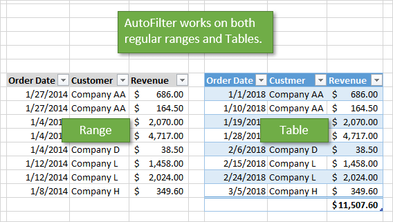
My preferred method is to use Tables because we don’t have to worry about changing range references as the table grows or shrinks. However, the code will be the same for both objects. The rest of the code examples use Excel tables, but you can easily modify this for regular ranges.
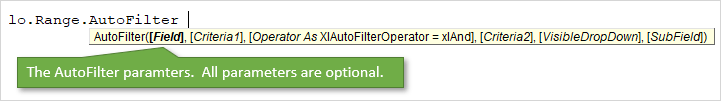
The 5 (or 6) AutoFilter Paramaters
The AutoFilter method has 5 (or 6) optional parameters that are used to specify the filter criteria for a column. Here is a list of the parameters.
| Name | Req/Opt | Description |
|---|---|---|
| Field | Optional | The number of the column within the filter range that the filter will be applied to. This is the column number within the filter range, NOT the column number of the worksheet. |
| Criteria1 | Optional | A string wrapped in quotation marks that is used to specify the filter criteria. Comparison operators can be included for less than or greater than filters. Many rules apply depending on the data type of the column. See examples below. |
| Operator | Optional | Specifies the type of filter for different data types and criteria by using one of the XlAutoFilterOperator constants. See this MSDN help page for a detailed list, and list in macro examples below. |
| Criteria2 | Optional | Used in combination with the Operator parameter and Criteria1 to create filters for multiple criteria or ranges. Also used for specific date filters for multiple items. |
| VisibleDropDown | Optional | Displays or hides the filter drop-down button for an individual column (field). |
| Subfield | Optional | Not sure yet… |
We can use a combination of these parameters to apply various filter criteria for different data types. The first four are the most important, so let’s take a look at how to apply those.
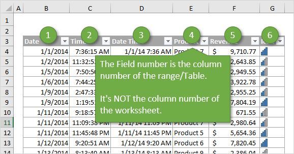
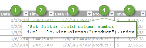
Step 2: The Field Parameter
The first parameter is the Field. For the Field parameter we specify a number that is the column number that the filter will be applied to. This is the column number within the filter range that is the parent of the AutoFilter method. It is NOT number of the column on the worksheet.
In the example below Field 4 is the Product column because it is the 4th column in the filter range/Table.
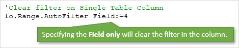
The column filter is cleared when we only specify the the Field parameter, and no other criteria.
We can also use a variable for the Field parameter and set it dynamically. I explain that in more detail below.
Step 3: The Criteria Parameters
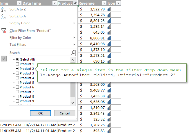
There are two parameters that can be used to specify the filter Criteria, Criteria1 and Criteria2. We use a combination of these parameters and the Operator parameter for different types of filters. This is where things get tricky, so let’s start with a simple example.
'Filter the Product column for a single item
lo.Range.AutoFilter Field:=4, Criteria1:="Product 2"
This would be the same as selecting a single item from the checkbox list in the filter drop-down menu.
General Rules for Criteria1 and Criteria2
The values we specify for Criteria1 and Criteria2 can get tricky. Here are some general guidelines for how to reference the Criteria parameter values.
- The criteria value is a string wrapped in quotation marks. There are a few exceptions where the criteria is a constant for date time period and above/below average.
- When specifying filters for single numbers or dates, the number formatting must match the number formatting that is applied in the range/table.
- The comparison operator for greater/less than is also included inside the quotation marks, before the number.
- Quotation marks are also used for filters for blanks “=” and non-blanks “<>”.
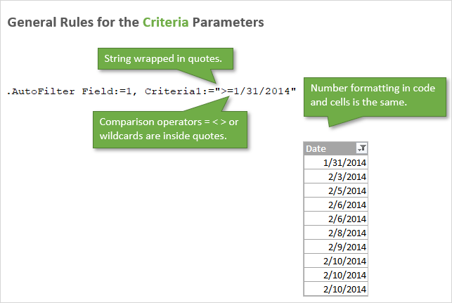
'Filter for date greater than or equal to Jan 1 2015
lo.Range.AutoFilter Field:=1, Criteria1:=">=1/1/2015"

' The comparison operator >= is inside the quotation marks
' for the Criteria1 parameter.

' The date formatting in the code matches the formatting
' applied to the cells in the worksheet.
Step 4: The Operator Parameter
What if we want to select multiple items from the filter drop-down? Or do a filter for a range of dates or numbers?
For this we need the Operator. The Operator parameter is used to specify what type of filter we want to apply. This can vary based on the type of data in the column. One of the following 11 constants must be used for the Operator.
| Name | Value | Description |
|---|---|---|
| xlAnd | 1 | Include both Criteria1 and Criteria2. Can be used for date or number ranges. |
| xlBottom10Items | 4 | Lowest-valued items displayed (number of items specified in Criteria1). |
| xlBottom10Percent | 6 | Lowest-valued items displayed (percentage specified in Criteria1). |
| xlFilterCellColor | 8 | Fill Color of the cell |
| xlFilterDynamic | 11 | Dynamic filter used for Above/Below Average and Date Periods |
| xlFilterFontColor | 9 | Color of the font in the cell |
| xlFilterIcon | 10 | Filter icon created by conditional formatting |
| xlFilterValues | 7 | Used for filters with multiple criteria specified with an Array function. |
| xlOr | 2 | Include either Criteria1 or Criteria2. Can be used for date and number ranges. |
| xlTop10Items | 3 | Highest-valued items displayed (number of items specified in Criteria1). |
| xlTop10Percent | 5 | Highest-valued items displayed (percentage specified in Criteria1). |
Here is a link to the MSDN help page that contains the list of constants for XlAutoFilterOperator Enumeration.
The operator is used in combination with Criteria1 and/or Criteria2, depending on the data type and filter type. Here are a few examples.
'Filter for list of multiple items, Operator is xlFilterValues
lo.Range.AutoFilter _
          Field:=iCol, _
          Criteria1:=Array("Product 4", "Product 5", "Product 6"), _
          Operator:=xlFilterValues
'Filter for Date Range (between dates), Operator is xlAnd
lo.Range.AutoFilter _
          Field:=iCol, _
          Criteria1:=">=1/1/2014", _
          Operator:=xlAnd, _
          Criteria2:="<=12/31/2015"
So that is the basics of writing a line of code for the AutoFilter method. It gets more complex with different data types. So I’ve provided many examples below that contain most of the combinations of Criteria and Operator for different types of filters.
AutoFilter is NOT Additive
When an AutoFilter line of code is run, it first clears any filters applied to that column (Field), then applies the filter criteria that is specified in the line of code.
This means it is NOT additive. The following 2 lines will NOT create a filter for Product 1 and Product 2. After the macro is run, the Product column will only be filtered for Product 2.
'AutoFilter is NOT addititive.  It first any filters applied
'in the column before applying the new filter
lo.Range.AutoFilter Field:=4, Criteria1:="Product 3"

'This line of code will filter the column for Product 2 only
'The filter for Product 3 above will be cleared when this line runs.
lo.Range.AutoFilter Field:=4, Criteria1:="Product 2"
If you want to apply a filter with multiple criteria to a single column, then you can specify that with the Criteria and Operator parameters.
How to Set the Field Number Dynamically
If we add/delete/move columns in the filter range, then the field number for a filtered column might change. Therefore, I try to avoid hard-coding a number for the Field parameter whenever possible.
We can use a variable instead and use some code to find the column number by it’s name. Here are two examples for regular ranges and Tables.
Sub Dynamic_Field_Number()
'Techniques to find and set the Field based on the column name.

Dim lo As ListObject
Dim iCol As Long

  'Set reference to the first Table on the sheet
  Set lo = Sheet1.ListObjects(1)

  'Set filter field
  iCol = lo.ListColumns("Product").Index

  'Use Match function for regular ranges
  'iCol = WorksheetFunction.Match("Product", Sheet1.Range("B3:G3"), 0)

  'Use the variable for the Field parameter value
  lo.Range.AutoFilter Field:=iCol, Criteria1:="Product 3"

End Sub
The column number will be found every time we run the macro. We don’t have to worry about changing the field number when the column moves. This saves time and prevents errors (win-win)! 🙂
Use Excel Tables with Filters
There are a lot of advantages to using Excel Tables, especially with the AutoFilter method. Here are a few of the major reasons I prefer Tables.
- We don’t have to redefine the range in VBA as the data range changes size (rows/columns are added/deleted). The entire Table is referenced with the ListObject object.
- It’s easy to reference the data in the Table after filters are applied. We can use the DataBodyRange property to reference visible rows to copy/paste, format, modify values, etc.
- We can have multiple Tables on the same sheet, and therefore multiple filter ranges. With regular ranges we can only have one filtered range per sheet.
- The code to clear all filters on a Table is easier to write.
Filters & Data Types
The filter drop-down menu options change based on what type of data is in the column. We have different filters for text, numbers, dates, and colors. This creates A LOT of different combinations of Operators and Criteria for each type of filter.
I created separate posts for each of these filter types. The posts contain explanations and VBA code examples.
- How to Clear Filters with VBA
- How to Filter for Blank & Non-Blank Cells
- How to Filter for Text with VBA
- How to Filter for Numbers with VBA
- How to Filter for Dates with VBA
- How to Filter for Colors & Icons with VBA
The file in the downloads section above contains all of these code samples in one place. You can add it to your Personal Macro Workbook and use the macros in your projects.
Why is the AutoFilter Method so Complex?
This post was inspired by a question from Chris, a member of The VBA Pro Course. The combinations of Criteria and Operators can be confusing and complex. Why is this?
Well, filters have evolved over the years. We saw a lot of new filter types introduced in Excel 2010, and the feature is continuing to be improved. However, the parameters of the AutoFilter method haven’t changed. This is great for compatibility with older versions, but also means the new filter types are being worked into the existing parameters.
Most of the filter code makes sense, but can be tricky to figure out at first. Fortunately we have the macro recorder to help with that.
I hope you can use this post and Excel file as a guide to writing macros for filters. Automating filters can save us and our users a ton of time, especially when using these techniques in a larger data automation project.
Please leave a comment below with any questions or suggestions. Thank you! 🙂
 In this Excel VBA Tutorial, you learn to filter data in Excel with macros.
This Excel VBA AutoFilter Tutorial is accompanied by an Excel workbook containing the data and macros I use in the examples below. You can get free access to this example workbook by clicking the button below.

Use the following Table of Contents to navigate to the Section you’re interested in.
Related Excel VBA and Macro Training Materials
The following VBA and Macro training materials may help you better understand and implement the contents below:
- Tutorials about general VBA constructs and structures:
- Tutorials for Beginners:
- Macro Tutorial for Beginners.
- VBA Tutorial for Beginners.
- Enable macros in Excel.
- Work with the Visual Basic Editor (VBE).
- Create Sub procedures.
- Refer to objects, including:
- Sheets.
- Cells.
- Work with properties and methods.
- Declare variables and data types.
- Create R1C1-style references.
- Use Excel worksheet functions in VBA.
- Work with arrays.
- Tutorials for Beginners:
- Tutorials with practical VBA applications and macro examples:
- Find last row.
- Set or get a cell’s value.
- Copy paste.
- Search and find.
- Create message boxes.
- The comprehensive and actionable Books at The Power Spreadsheets Library:
- Excel Macros for Beginners Book Series.
- VBA Fundamentals Book Series.
#1. Excel VBA AutoFilter Column Based on Cell Value
VBA Code to AutoFilter Column Based on Cell Value
To AutoFilter a column based on a cell value, use the following structure/template in the applicable statement:
RangeObjectColumnToFilter.AutoFilter Field:=1, Criteria1:="ComparisonOperator" & RangeObjectCriteria.Value
The following Sections describe the main elements in this structure.
RangeObjectColumnToFilter
A Range object representing the column you AutoFilter.
AutoFilter
The Range.AutoFilter method filters a list with Excel’s AutoFilter.
Field:=1
The Field parameter of the Range.AutoFilter method:
- Specifies the field offset (column number) on which you base the AutoFilter.
- Is specified as an integer, with the first/leftmost column in the AutoFiltered cell range (RangeObjectColumnToFilter) being field 1.
To AutoFilter a column based on a cell value, set the Field parameter to 1.
Criteria1:=”ComparisonOperator” & RangeObjectCriteria.Value
The Criteria1 parameter of the Range.AutoFilter method is:
- As a general rule, a string specifying the AutoFiltering criteria.
- Subject to a variety of rules. The specific rules (usually) depend on the data type of the AutoFiltered column.
To AutoFilter a column based on a cell value (and as a general rule), set the Criteria1 parameter to a string specifying the AutoFiltering criteria by specifying:
- A comparison operator (ComparisonOperator); and
- The cell (RangeObjectCriteria) whose value you use to AutoFilter the column.
For these purposes:
- “ComparisonOperator” is a comparison operator specifying the type of comparison VBA carries out.
- “&” is the concatenation operator.
- “RangeObjectCriteria” is a Range object representing the cell whose value you use to AutoFilter the column (RangeObjectColumnToFilter).
- “Value” refers to the Range.Value property. The Range.Value property returns the value/string stored in the applicable cell (RangeObjectCriteria).
Macro Example to AutoFilter Column Based on Cell Value
The macro below does the following:
- Filter column A (with the data set starting in cell A6) of the worksheet named “AutoFilter Column Cell Value” in the workbook where the procedure is stored.
- Display (only) entries whose value is not equal to the value stored in cell D6 of the worksheet named “AutoFilter Column Cell Value” in the workbook where the procedure is stored.
Sub AutoFilterColumnCellValue()
    'Source: https://powerspreadsheets.com/
    'For further information: https://powerspreadsheets.com/excel-vba-autofilter/

    'This procedure:
        '(1) Filters the column/data starting on cell A6 of the "AutoFilter Column Cell Value" worksheet in this workbook based on the value stored in cell D6 of the same worksheet
        '(2) Displays (only) entries whose value is not equal to (<>) the value stored in cell D6 of the "AutoFilter Column Cell Value" worksheet in this workbook

    With ThisWorkbook.Worksheets("AutoFilter Column Cell Value")
        .Range("A6").AutoFilter Field:=1, Criteria1:="<>" & .Range("D6").Value
    End With

End Sub
Effects of Executing Macro Example to AutoFilter Column Based on Cell Value
The image below illustrates the effects of using the macro example. In this example:
- Column A (cells A6 to A31) contains:
- A header (cell A6); and
- Randomly generated values (cells A7 to A31).
- Cell D6 contains a randomly generated value (8).
- A text box (Filter column A based on value of cell D6) executes the macro example when clicked.
When the macro is executed, Excel:
- Filters column A based on the value in cell D6.
- Displays (only) entries whose value is not equal to the value in cell D6 (8).

#2. Excel VBA AutoFilter Table Based on 1 Column and 1 Cell Value
VBA Code to AutoFilter Table Based on 1 Column and 1 Cell Value
To AutoFilter a table based on 1 column and 1 cell value, use the following structure/template in the applicable statement:
RangeObjectTableToFilter.AutoFilter Field:=ColumnCriteria, Criteria1:="ComparisonOperator" & RangeObjectCriteria.Value
The following Sections describe the main elements in this structure.
RangeObjectTableToFilter
A Range object representing the table you AutoFilter.
AutoFilter
The Range.AutoFilter method filters a list with Excel’s AutoFilter.
Field:=ColumnCriteria
The Field parameter of the Range.AutoFilter method:
- Specifies the field offset (column number) on which you base the AutoFilter.
- Is specified as an integer, with the first/leftmost column in the AutoFiltered cell range (RangeObjectTableToFilter) being field 1.
To AutoFilter a table based on 1 column and 1 cell value, set the Field parameter to an integer specifying the number of the column (in RangeObjectTableToFilter) you use to AutoFilter the table.
Criteria1:=”ComparisonOperator” & RangeObjectCriteria.Value
The Criteria1 parameter of the Range.AutoFilter method is:
- As a general rule, a string specifying the AutoFiltering criteria.
- Subject to a variety of rules. The specific rules (usually) depend on the data type of the AutoFiltered column (ColumnCriteria).
To AutoFilter a table based on 1 column and 1 cell value (and as a general rule), set the Criteria1 parameter to a string specifying the AutoFiltering criteria by specifying:
- A comparison operator (ComparisonOperator); and
- The cell (RangeObjectCriteria) whose value you use to AutoFilter the table.
For these purposes:
- “ComparisonOperator” is a comparison operator specifying the type of comparison VBA carries out.
- “&” is the concatenation operator.
- “RangeObjectCriteria” is a Range object representing the cell whose value you use to AutoFilter the table (RangeObjectTableToFilter).
- “Value” refers to the Range.Value property. The Range.Value property returns the value/string stored in the applicable cell (RangeObjectCriteria).
Macro Example to AutoFilter Table Based on 1 Column and 1 Cell Value
The macro below does the following:
- Filter the table stored in cells A6 to H31 of the worksheet named “AutoFilter Table Column Value” in the workbook where the procedure is stored based on:
- The table’s fourth column; and
- The value stored in cell K6 of the same worksheet.
- Display (only) entries whose value in the fourth column of the AutoFiltered table is greater than or equal to the value stored in cell K6 of the worksheet named “AutoFilter Table Column Value” in the workbook where the procedure is stored.
Sub AutoFilterTable1Column1CellValue()
    'Source: https://powerspreadsheets.com/
    'For further information: https://powerspreadsheets.com/excel-vba-autofilter/

    'This procedure:
        '(1) Filters the table in cells A6 to H31 of the "AutoFilter Table Column Value" worksheet in this workbook based on:
            'It's fourth column; and
            'The value stored in cell K6 of the same worksheet
        '(2) Displays (only) entries in rows where the value in the fourth table column is greater than or equal to (>=) the value stored in cell K6 of the "AutoFilter Table Column Value" worksheet in this workbook

    With ThisWorkbook.Worksheets("AutoFilter Table Column Value")
        .Range("A6:H31").AutoFilter Field:=4, Criteria1:=">=" & .Range("K6").Value
    End With

End Sub
Effects of Executing Macro Example to AutoFilter Table Based on 1 Column and 1 Cell Value
The image below illustrates the effects of using the macro example. In this example:
- Columns A through H (cells A6 to H31) contain a table organized as follows:
- A header row (cells A6 to H6); and
- Randomly generated values (cells A7 to H31).
- Cell K6 contains a randomly generated value (8).
- A text box (Filter table based on Column 4 and value of cell K6) executes the macro example when clicked.
When the macro is executed, Excel:
- Filters the table based on:
- Column 4; and
- The value in cell K6.
- Displays (only) entries whose value in Column 4 is greater than or equal to the value in cell K6 (8).

#3. Excel VBA AutoFilter Table by Column Header Name
VBA Code to AutoFilter Table by Column Header Name
To AutoFilter a table by column header name, use the following structure/template in the applicable procedure:
With RangeObjectTableToFilter
    ColumnNumberVariable = .Rows(1).Find(What:=ColumnHeaderName, LookIn:=XlFindLookInConstant, LookAt:=XlLookAtConstant, SearchOrder:=xlByColumns, SearchDirection:=xlNext).Column - .Column + 1
    .AutoFilter Field:=ColumnNumberVariable, Criteria1:=AutoFilterCriterion
End With
The following Sections describe the main elements in this structure.
Lines #1 and #4: With RangeObjectTableToFilter | End With
With RangeObjectTableToFilter
The With statement (With) executes a set of statements (lines #2 and #3) on the object you refer to (RangeObjectTableToFilter).
“RangeObjectTableToFilter” is a Range object representing the table you AutoFilter.
End With
The End With statement (End With) ends a With… End With block.
Line #2: ColumnNumberVariable = .Rows(1).Find(What:=ColumnHeaderName, LookIn:=XlFindLookInConstant, LookAt:=XlLookAtConstant, SearchOrder:=xlByColumns, SearchDirection:=xlNext).Column – .Column + 1
ColumnNumberVariable
Variable of (usually) the Long data type holding/representing the number of the column (in RangeObjectTableToFilter) whose column header name (ColumnHeaderName) you use to AutoFilter the table.
=
The assignment operator assigns a value (.Rows(1).Find(What:=ColumnHeaderName, LookIn:=XlFindLookInConstant, LookAt:=XlLookAtConstant, SearchOrder:=xlByColumns, SearchDirection:=xlNext).Column – .Column + 1) to a variable (ColumnNumberVariable).
.Rows(1).Find(What:=ColumnHeaderName, LookIn:=XlFindLookInConstant, LookAt:=XlLookAtConstant, SearchOrder:=xlByColumns, SearchDirection:=xlNext).Column – .Column + 1
The expression whose value you assign to the ColumnNumberVariable.
Rows(1)
The Range.Rows property (Rows) returns a Range object representing all rows in the applicable cell range (RangeObjectTableToFilter).
The Range.Item property (1) returns a Range object representing the first (1) row in the cell range represented by the applicable Range object (returned by the Range.Rows property).
Find(What:=ColumnHeaderName, LookIn:=XlFindLookInConstant, LookAt:=XlLookAtConstant, SearchOrder:=xlByColumns, SearchDirection:=xlNext)
The Range.Find method:
- Finds specific information (the column header name) in a cell range (Rows(1)).
- Returns a Range object representing the first cell where the information is found.
What:=ColumnHeaderName
The What parameter of the Range.Find method specifies the data to search for.
To find the header name of the column you use to AutoFilter a table, set the What parameter to the header name of the column you use to AutoFilter the table (ColumnHeaderName).
LookIn:=XlFindLookInConstant
The LookIn parameter of the Range.Find method:
- Specifies the type of data to search in.
- Can take any of the built-in constants or values from the XlFindLookIn enumeration.
To find the header name of the column you use to AutoFilter a table, set the LookIn parameter to either of the following, as applicable:
- xlFormulas (LookIn:=xlFormulas): To search in the applicable cell range’s formulas.
- xlValues (LookIn:=xlValues): To search in the applicable cell range’s values.
LookAt:=XlLookAtConstant
The LookAt parameter of the Range.Find method:
- Specifies against which of the following the data you are searching for is matched:
- The entire/whole searched cell contents.
- Any part of the searched cell contents.
- Can take any of the built-in constants or values from the XlLookAt enumeration.
To find the header name of the column you use to AutoFilter a table, set the LookAt parameter to either of the following, as applicable:
- xlWhole (LookAt:=xlWhole): To match against the entire/whole searched cell contents.
- xlPart (LookAt:=xlPart): To match against any part of the searched cell contents.
SearchOrder:=xlByColumns
The SearchOrder parameter of the Range.Find method:
- Specifies the order in which the applicable cell range (Rows(1)) is searched:
- By rows.
- By columns.
- Can take any of the built-in constants or values from the XlSearchOrder enumeration.
To find the header name of the column you use to AutoFilter a table, set the SearchOrder parameter to xlByColumns. xlByColumns searches by columns.
SearchDirection:=xlNext
The SearchDirection parameter of the Range.Find method:
- Specifies the search direction:
- Search for the previous match.
- Search for the next match.
- Can take any of the built-in constants or values from the XlSearchDirection enumeration.
To find the header name of the column you use to AutoFilter a table, set the SearchDirection parameter to xlNext. xlNext searches for the next match.
Column
The Range.Column property returns the number of the first column of the first area in a cell range.
When AutoFiltering a table by column header name, the Range.Column property returns the 2 following column numbers:
- The column number of the cell represented by the Range object returned by the Range.Find method (Find(What:=ColumnHeaderName, LookIn:=XlFindLookInConstant, LookAt:=XlLookAtConstant, SearchOrder:=xlByColumns, SearchDirection:=xlNext)).
- The number of the first column in the table you AutoFilter (RangeObjectTableToFilter).
– .Column + 1
The number of the column you use to AutoFilter the table may vary depending on which of the following you use as reference (to calculate such column number):
- The entire worksheet. From this perspective:
- Column A is column #1.
- Column B is column #2.
- …
- And so on.
- The table you AutoFilter. From this perspective:
- The first table column is column #1.
- The second table column is column #2.
- …
- And so on.
As a general rule:
- The column numbers will match if the first column of the table you AutoFilter (RangeObjectTableToFilter) is column A of the applicable worksheet.
- The column numbers will not match if the first column of the table you AutoFilter (RangeObjectTableToFilter) is not column A of the applicable worksheet.
The Range.Column property (Column) uses the entire worksheet as reference. The Range.AutoFilter method (line #3) uses the table you AutoFilter as reference.
The following ensures the column numbers (returned by the Range.Column property and used by the Range.AutoFilter method) match, regardless of which worksheet column is the first column of the table you AutoFilter:
- Subtract the number of the first column in the table you AutoFilter (RangeObjectTableToFilter) from the column number of the cell represented by the Range object returned by the Range.Find method (- .Column); and
- Add 1 (+ 1).
Line #3: .AutoFilter Field:=ColumnNumberVariable, Criteria1:=AutoFilterCriterion
AutoFilter
The Range.AutoFilter method filters a list with Excel’s AutoFilter.
Field:=ColumnNumberVariable
The Field parameter of the Range.AutoFilter method:
- Specifies the field offset (column number) on which you base the AutoFilter.
- Is specified as an integer, with the first/leftmost column in the AutoFiltered cell range (RangeObjectTableToFilter) being field 1.
To AutoFilter a table by column header name, set the Field parameter to the number of the column (in RangeObjectTableToFilter) whose column header name you use to AutoFilter the table (ColumnNumberVariable).
Criteria1:=AutoFilterCriterion
The Criteria1 parameter of the Range.AutoFilter method is:
- As a general rule, a string specifying the AutoFiltering criteria.
- Subject to a variety of rules. The specific rules (usually) depend on the data type of the AutoFiltered column (ColumnNumberVariable).
To AutoFilter a table by column header name (and as a general rule), set the Criteria1 parameter to a string specifying the AutoFiltering criteria (AutoFilterCriterion) by specifying:
- A comparison operator; and
- The applicable criterion you use to AutoFilter the table.
Macro Example to AutoFilter Table by Column Header Name
The macro below does the following:
- Filter the table starting on cell B6 of the worksheet named “AutoFilter Table Column Name” in the workbook where the procedure is stored based on the column whose header name is “Column 4”.
- Display (only) entries in rows where the value in the table column whose column header name is “Column 4” is greater than or equal to 8.
Sub AutoFilterTableColumnHeaderName()
    'Source: https://powerspreadsheets.com/
    'For further information: https://powerspreadsheets.com/excel-vba-autofilter/

    'This procedure:
        '(1) Filters the table starting on cell B6 of the "AutoFilter Table Column Name" worksheet in this workbook based on the column whose header name is "Column 4"
        '(2) Displays (only) entries in rows where the value in the table column whose column header name is "Column 4" is greater than or equal to (>=) 8

    'Declare object variable to represent the cell range of the AutoFiltered table
    Dim MyAutoFilteredTable As Range

    'Declare variable to hold/represent the number of the column (in the AutoFiltered table) whose column header name is "Column 4"
    Dim MyColumnNumber As Long

    'Assign an object reference (representing the cell range of the AutoFiltered table) to the MyAutoFilteredTable object variable
    Set MyAutoFilteredTable = ThisWorkbook.Worksheets("AutoFilter Table Column Name").Range("B6").CurrentRegion

    'Refer to the cell range represented by the MyAutoFilteredTable object variable
    With MyAutoFilteredTable

        'Assign the number of the column (in the AutoFiltered table) whose column header name is "Column 4" to the MyColumnNumber variable
        MyColumnNumber = .Rows(1).Find(What:="Column 4", LookIn:=xlFormulas, LookAt:=xlWhole, SearchOrder:=xlByColumns, SearchDirection:=xlNext).Column - .Column + 1

        'Filter the AutoFiltered table based on the column whose number is held/represented by the MyColumnNumber variable (the column whose header name is "Column 4")
        .AutoFilter Field:=MyColumnNumber, Criteria1:=">=8"

    End With

End Sub
Effects of Executing Macro Example to AutoFilter Table by Column Name
The image below illustrates the effects of using the macro example. In this example:
- Columns B through I (cells B6 to I31) contain a table organized as follows:
- A header row (cells B6 to I6); and
- Randomly generated values (cells B7 to I31).
- A text box (Filter table by Column 4) executes the macro example when clicked.
When the macro is executed, Excel:
- Filters the table based on Column 4.
- Displays (only) entries whose value in Column 4 is greater than or equal to 8.

#4. Excel VBA AutoFilter Excel Table by Column Header Name
VBA Code to AutoFilter Excel Table by Column Header Name
To AutoFilter an Excel Table by column header name, use the following structure/template in the applicable statement:
ListObjectObject.Range.AutoFilter Field:=ListObjectObject.ListColumns(ColumnHeaderName).Index, Criteria1:=AutoFilterCriterion
The following Sections describe the main elements in this structure.
ListObjectObject
A ListObject object representing the Excel Table you AutoFilter.
Range
The ListObject.Range property returns a Range object representing the cell range to which the applicable Excel Table (ListObjectObject) applies.
AutoFilter Field:=ListObjectObject.ListColumns(ColumnHeaderName).Index, Criteria1:=AutoFilterCriterion
AutoFilter
The Range.AutoFilter method filters a list with Excel’s AutoFilter.
Field:=ListObjectObject.ListColumns(ColumnHeaderName).Index
The Field parameter of the Range.AutoFilter method:
- Specifies the field offset (column number) on which you base the AutoFilter.
- Is specified as an integer, with the first/leftmost column in the AutoFiltered cell range (ListObjectObject.Range) being field 1.
To AutoFilter an Excel Table by column header name, set the Field parameter to the number of the column (in the applicable Excel Table) whose column header name you use to AutoFilter the Excel Table. For these purposes:
- “ListObjectObject” is a ListObject object representing the Excel Table you AutoFilter.
- The ListObject.ListColumns property (ListColumns) returns a ListColumns collection representing all columns in the applicable Excel Table (ListObjectObject).
- The ListColumns.Item property (ColumnHeaderName) returns a ListColumn object representing the column whose header name (ColumnHeaderName) you use to AutoFilter the Excel Table (ListObjectObject).
- “ColumnHeaderName” is the header name of the column you use to AutoFilter the Excel Table (ListObjectObject).
- The ListColumn.Index property (Index) returns a Long value representing the index (column) number of the column (whose header name is ColumnHeaderName) you use to AutoFilter the Excel Table (ListObjectObject).
Criteria1:=AutoFilterCriterion
The Criteria1 parameter of the Range.AutoFilter method is:
- As a general rule, a string specifying the AutoFiltering criteria.
- Subject to a variety of rules. The specific rules (usually) depend on the data type of the AutoFiltered column.
To AutoFilter an Excel Table by column header name (and as a general rule), set the Criteria1 parameter to a string specifying the AutoFiltering criteria (AutoFilterCriterion) by specifying:
- A comparison operator; and
- The applicable criterion you use to AutoFilter the Excel Table.
Macro Example to AutoFilter Excel Table by Column Header Name
The macro below does the following:
- Filter the Excel Table named “Table1” in the worksheet named “AutoFilter Excel Table Column” in the workbook where the procedure is stored based on the column whose header name is “Column 4”.
- Display (only) entries in rows where the value in the Excel Table column whose column header name is “Column 4” is greater than or equal to 8.
Sub AutoFilterExcelTableColumnHeaderName()
    'Source: https://powerspreadsheets.com/
    'For further information: https://powerspreadsheets.com/excel-vba-autofilter/

    'This procedure:
        '(1) Filters the "Table1" Excel Table in the "AutoFilter Excel Table Column" worksheet in this workbook based on the column whose header name is "Column 4"
        '(2) Displays (only) entries in rows where the value in the Excel Table column whose column header name is "Column 4" is greater than or equal to (>=) 8

    With ThisWorkbook.Worksheets("AutoFilter Excel Table Column").ListObjects("Table1")
        .Range.AutoFilter Field:=.ListColumns("Column 4").Index, Criteria1:=">=8"
    End With

End Sub
Effects of Executing Macro Example to AutoFilter Excel Table by Column Name
The image below illustrates the effects of using the macro example. In this example:
- Columns B through I (cells B6 to I31) contain an Excel Table (Table1) organized as follows:
- A header row (cells B6 to I6); and
- Randomly generated values (cells B7 to I31).
- A text box (Filter Excel Table by Column 4) executes the macro example when clicked.
When the macro is executed, Excel:
- Filters the Excel Table (Table1) based on Column 4.
- Displays (only) entries whose value in Column 4 is greater than or equal to 8.

#5. Excel VBA AutoFilter with Multiple Criteria in Same Column (or Field) and Exact Matches
VBA Code to AutoFilter with Multiple Criteria in Same Column (or Field) and Exact Matches
To AutoFilter with multiple criteria in the same column (or field) and consider exact matches, use the following structure/template in the applicable statement:
RangeObjectToFilter.AutoFilter Field:=ColumnNumber, Criteria1:=ArrayMultipleCriteria, Operator:=xlFilterValues
The following Sections describe the main elements in this structure.
RangeObjectToFilter
A Range object representing the data set you AutoFilter.
AutoFilter
The Range.AutoFilter method filters a list with Excel’s AutoFilter.
Field:=ColumnNumber
The Field parameter of the Range.AutoFilter method:
- Specifies the field offset (column number) on which you base the AutoFilter.
- Is specified as an integer, with the first/leftmost column in the AutoFiltered cell range (RangeObjectToFilter) being field 1.
To AutoFilter with multiple criteria in the same column (or field) and consider exact matches, set the Field parameter to an integer specifying the number of the column (in RangeObjectToFilter) you use to AutoFilter the data set.
Criteria1:=ArrayMultipleCriteria
The Criteria1 parameter of the Range.AutoFilter method is:
- As a general rule, a string specifying the AutoFiltering criteria.
- Subject to a variety of rules. The specific rules (usually) depend on the data type of the AutoFiltered column (ColumnNumber).
To AutoFilter with multiple criteria in the same column (or field) and consider exact matches, set the Criteria1 parameter to an array. Each individual array element is (as a general rule) a string specifying an individual AutoFiltering criterion.
Operator:=xlFilterValues
The Operator parameter of the Range.AutoFilter method:
- Specifies the type of AutoFilter.
- Can take any of the built-in constants or values from the XlAutoFilterOperator enumeration.
To AutoFilter with multiple criteria in the same column (or field) and consider exact matches, set the Operator parameter to xlFilterValues. xlFilterValues refers to values.
Macro Example to AutoFilter with Multiple Criteria in Same Column (or Field) and Exact Matches
The macro below does the following:
- Filter column A (with the data set starting in cell A6) of the worksheet named “AutoFilter Mult Criteria Column” in the workbook where the procedure is stored.
- Display (only) entries whose value is equal to one of the values stored in column C (with the AutoFiltering criteria starting in cell C7) of the worksheet named “AutoFilter Mult Criteria Column” in the workbook where the procedure is stored.
Sub AutoFilterMultipleCriteriaSameColumnExactMatch()
    'Source: https://powerspreadsheets.com/
    'For further information: https://powerspreadsheets.com/excel-vba-autofilter/

    'This procedure:
        '(1) Filters the column/data starting on cell A6 of the "AutoFilter Mult Criteria Column" worksheet in this workbook based on the multiple criteria/values stored in the column starting on cell C7 of the same worksheet
        '(2) Displays (only) entries whose value is equal to one of the multiple values/criteria stored in the column starting on cell C7 of the "AutoFilter Mult Criteria Column" worksheet in this workbook

    'Declare array to hold/represent multiple criteria
    Dim MyArray As Variant

    'Identify worksheet with (i) data to AutoFilter, and (ii) multiple AutoFiltering criteria
    With ThisWorkbook.Worksheets("AutoFilter Mult Criteria Column")

        'Fill MyArray with values/criteria stored in the column starting on cell C7
        MyArray = Split(Join(Application.Transpose(.Range(.Cells(7, 3), .Cells(.Range("C:C").Find(What:="*", LookIn:=xlFormulas, LookAt:=xlPart, SearchOrder:=xlByRows, SearchDirection:=xlPrevious).Row, 3)).Value)))

        'Filter column/data starting on cell A6 based on the multiple criteria/values held/represented by MyArray
        .Range("A6").AutoFilter Field:=1, Criteria1:=MyArray, Operator:=xlFilterValues

    End With

End Sub
Effects of Executing Macro Example to AutoFilter with Multiple Criteria in Same Column (or Field) and Exact Matches
The image below illustrates the effects of using the macro example. In this example:
- Column A (cells A6 to H31) contains:
- A header (cell A6); and
- Randomly generated values (cells A7 to A31).
- Column C (cells C7 to C11) contains even numbers between (and including):
- 2; and
- 10.
- A text box (Filter column A based on values in column C) executes the macro example when clicked.
When the macro is executed, Excel:
- Filters column A based on the multiple criteria/values in column C.
- Displays (only) entries whose value is equal to one of the values stored in column C (2, 4, 6, 8, 10).

#6. Excel VBA AutoFilter with Multiple Criteria and xlAnd Operator
VBA Code to AutoFilter with Multiple Criteria and xlAnd Operator
To AutoFilter with multiple criteria and the xlAnd operator, use the following structure/template in the applicable statement:
RangeObjectToFilter.AutoFilter Field:=ColumnNumber, Criteria1:="ComparisonOperator" & FilteringCriterion1, Operator:=xlAnd, Criteria2:="ComparisonOperator" & FilteringCriterion2
The following Sections describe the main elements in this structure.
RangeObjectToFilter
A Range object representing the data set you AutoFilter.
AutoFilter
The Range.AutoFilter method filters a list with Excel’s AutoFilter.
Field:=ColumnNumber
The Field parameter of the Range.AutoFilter method:
- Specifies the field offset (column number) on which you base the AutoFilter.
- Is specified as an integer, with the first/leftmost column in the AutoFiltered cell range (RangeObjectToFilter) being field 1.
To AutoFilter with multiple criteria and the xlAnd operator, set the Field parameter to an integer specifying the number of the column (in RangeObjectToFilter) you use to AutoFilter the data set.
Criteria1:=”ComparisonOperator” & FilteringCriterion1
The Criteria1 parameter of the Range.AutoFilter method is:
- As a general rule, a string specifying the first AutoFiltering criterion.
- Subject to a variety of rules. The specific rules (usually) depend on the data type of the AutoFiltered column (ColumnNumber).
To AutoFilter with multiple criteria and the xlAnd operator (and as a general rule), set the Criteria1 parameter to a string specifying the first AutoFiltering criterion by specifying:
- A comparison operator (ComparisonOperator); and
- The applicable criterion you use to AutoFilter the data set.
For these purposes:
- “ComparisonOperator” is a comparison operator specifying the type of comparison VBA carries out.
- “&” is the concatenation operator.
- “FilteringCriterion1” is the first criterion (for example, a value) you use to AutoFilter the data set (RangeObjectToFilter).
Operator:=xlAnd
The Operator parameter of the Range.AutoFilter method:
- Specifies the type of AutoFilter.
- Can take any of the built-in constants or values from the XlAutoFilterOperator enumeration.
To AutoFilter with multiple criteria and the xlAnd operator, set the Operator parameter to xlAnd. xlAnd refers to the logical And operator (logical conjunction of Criteria1 and Criteria2).
Criteria2:=”ComparisonOperator” & FilteringCriterion2
The Criteria2 parameter of the Range.AutoFilter method is:
- As a general rule, a string specifying the second AutoFiltering criterion.
- Subject to a variety of rules. The specific rules (usually) depend on the data type of the AutoFiltered column (ColumnNumber).
To AutoFilter with multiple criteria and the xlAnd operator (and as a general rule), set the Criteria2 parameter to a string specifying the second AutoFiltering criterion by specifying:
- A comparison operator (ComparisonOperator); and
- The applicable criterion you use to AutoFilter the data set.
For these purposes:
- “ComparisonOperator” is a comparison operator specifying the type of comparison VBA carries out.
- “&” is the concatenation operator.
- “FilteringCriterion2” is the second criterion (for example, a value) you use to AutoFilter the data set (RangeObjectToFilter).
Macro Example to AutoFilter with Multiple Criteria and xlAnd Operator
The macro below does the following:
- Filter column A (with the data set starting in cell A6) of the worksheet named “AutoFilter Mult Criteria xlAnd” in the workbook where the procedure is stored.
- Display (only) entries whose value is greater than or equal to (>=) the criterion/value stored in cell D6 and (xlAnd) less than or equal to (<=) the criterion/value stored in cell D7 of the worksheet named “AutoFilter Mult Criteria xlAnd” in the workbook where the procedure is stored.
Sub AutoFilterMultipleCriteriaXlAnd()
    'Source: https://powerspreadsheets.com/
    'For further information: https://powerspreadsheets.com/excel-vba-autofilter/

    'This procedure:
        '(1) Filters the column/data starting on cell A6 of the "AutoFilter Mult Criteria xlAnd" worksheet in this workbook based on the multiple criteria/values stored in cells D6 and (xlAnd) D7 of the same worksheet
        '(2) Displays (only) entries whose value is greater than or equal to (>=) the criterion/value stored in cell D6 and (xlAnd) less than or equal to (<=) the criterion/value stored in cell D7 of the "AutoFilter Mult Criteria xlAnd" worksheet in this workbook

    'Identify worksheet with (i) data to AutoFilter, and (ii) multiple AutoFiltering criteria (xlAnd)
    With ThisWorkbook.Worksheets("AutoFilter Mult Criteria xlAnd")

        'Filter column/data starting on cell A6 based on the multiple criteria/values stored in cells D6 and (xlAnd) D7
        .Range("A6").AutoFilter Field:=1, Criteria1:=">=" & .Range("D6").Value, Operator:=xlAnd, Criteria2:="<=" & .Range("D7").Value

    End With

End Sub
Effects of Executing Macro Example to AutoFilter with Multiple Criteria and xlAnd Operator
The image below illustrates the effects of using the macro example. In this example:
- Column A (cells A6 to H31) contains:
- A header (cell A6); and
- Randomly generated values (cells A7 to A31).
- Cells D6 and D7 contain values (10 and 15).
- A text box (Filter column A based on maximum and (xlAnd) minimum values) executes the macro example when clicked.
When the macro is executed, Excel:
- Filters column A based on the multiple criteria/values in cells D6 and D7.
- Displays (only) entries whose value is between the values stored in cells D6 (minimum 10) and (xlAnd) D7 (maximum 15).

#7. Excel VBA AutoFilter with Multiple Criteria and xlOr Operator
VBA Code to AutoFilter with Multiple Criteria and xlOr Operator
To AutoFilter with multiple criteria and the xlOr operator, use the following structure/template in the applicable statement:
RangeObjectToFilter.AutoFilter Field:=ColumnNumber, Criteria1:="ComparisonOperator" & FilteringCriterion1, Operator:=xlOr, Criteria2:="ComparisonOperator" & FilteringCriterion2
The following Sections describe the main elements in this structure.
RangeObjectToFilter
A Range object representing the data set you AutoFilter.
AutoFilter
The Range.AutoFilter method filters a list with Excel’s AutoFilter.
Field:=ColumnNumber
The Field parameter of the Range.AutoFilter method:
- Specifies the field offset (column number) on which you base the AutoFilter.
- Is specified as an integer, with the first/leftmost column in the AutoFiltered cell range (RangeObjectToFilter) being field 1.
To AutoFilter with multiple criteria and the xlOr operator, set the Field parameter to an integer specifying the number of the column (in RangeObjectToFilter) you use to AutoFilter the data set.
Criteria1:=”ComparisonOperator” & FilteringCriterion1
The Criteria1 parameter of the Range.AutoFilter method is:
- As a general rule, a string specifying the first AutoFiltering criterion.
- Subject to a variety of rules. The specific rules (usually) depend on the data type of the AutoFiltered column (ColumnNumber).
To AutoFilter with multiple criteria and the xlOr operator (and as a general rule), set the Criteria1 parameter to a string specifying the first AutoFiltering criterion by specifying:
- A comparison operator (ComparisonOperator); and
- The applicable criterion you use to AutoFilter the data set.
For these purposes:
- “ComparisonOperator” is a comparison operator specifying the type of comparison VBA carries out.
- “&” is the concatenation operator.
- “FilteringCriterion1” is the first criterion (for example, a value) you use to AutoFilter the data set (RangeObjectToFilter).
Operator:=xlOr
The Operator parameter of the Range.AutoFilter method:
- Specifies the type of AutoFilter.
- Can take any of the built-in constants or values from the XlAutoFilterOperator enumeration.
To AutoFilter with multiple criteria and the xlOr operator, set the Operator parameter to xlOr. xlOr refers to the logical Or operator (logical disjunction of Criteria1 and Criteria2).
Criteria2:=”ComparisonOperator” & FilteringCriterion2
The Criteria2 parameter of the Range.AutoFilter method is:
- As a general rule, a string specifying the second AutoFiltering criterion.
- Subject to a variety of rules. The specific rules (usually) depend on the data type of the AutoFiltered column (ColumnNumber).
To AutoFilter with multiple criteria and the xlOr operator (and as a general rule), set the Criteria2 parameter to a string specifying the second AutoFiltering criterion by specifying:
- A comparison operator (ComparisonOperator); and
- The applicable criterion you use to AutoFilter the data set.
For these purposes:
- “ComparisonOperator” is a comparison operator specifying the type of comparison VBA carries out.
- “&” is the concatenation operator.
- “FilteringCriterion2” is the second criterion (for example, a value) you use to AutoFilter the data set (RangeObjectToFilter).
Macro Example to AutoFilter with Multiple Criteria and xlOr Operator
The macro below does the following:
- Filter column A (with the data set starting in cell A6) of the worksheet named “AutoFilter Mult Criteria xlOr” in the workbook where the procedure is stored.
- Display (only) entries whose value is either:
- Less than (<) the criterion/value stored in cell D6 of the worksheet named “AutoFilter Mult Criteria xlOr” in the workbook where the procedure is stored; or (xlOr)
- Greater than (>) the criterion value stored in cell D7 of the worksheet named “AutoFilter Mult Criteria xlOr” in the workbook where the procedure is stored.
Sub AutoFilterMultipleCriteriaXlOr()
    'Source: https://powerspreadsheets.com/
    'For further information: https://powerspreadsheets.com/excel-vba-autofilter/

    'This procedure:
        '(1) Filters the column/data starting on cell A6 of the "AutoFilter Mult Criteria xlOr"" worksheet in this workbook based on the multiple criteria/values stored in cells D6 or (xlOr) D7 of the same worksheet
        '(2) Displays (only) entries whose value is less than (<) the criterion/value stored in cell D6 or (xlOr) greater than (>) the criterion/value stored in cell D7 of the "AutoFilter Mult Criteria xlOr" worksheet in this workbook

    'Identify worksheet with (i) data to AutoFilter, and (ii) multiple AutoFiltering criteria (xlOr)
    With ThisWorkbook.Worksheets("AutoFilter Mult Criteria xlOr")

        'Filter column/data starting on cell A6 based on the multiple criteria/values stored in cells D6 or (xlOr) D7
        .Range("A6").AutoFilter Field:=1, Criteria1:="<" & .Range("D6").Value, Operator:=xlOr, Criteria2:=">" & .Range("D7").Value

    End With

End Sub
Effects of Executing Macro Example to AutoFilter with Multiple Criteria and xlOr Operator
The image below illustrates the effects of using the macro example. In this example:
- Column A (cells A6 to H31) contains:
- A header (cell A6); and
- Randomly generated values (cells A7 to A31).
- Cells D6 and D7 contain values (10 and 15).
- A text box (Filter column A based on criteria in column D (xlOr)) executes the macro example when clicked.
When the macro is executed, Excel:
- Filters column A based on the multiple criteria/values in cells D6 and D7.
- Displays (only) entries whose value is:
- Less than the value stored in cell D6 (10); or (xlOr)
- Greater than the value stored in cell D7 (15).

#8. Excel VBA AutoFilter Multiple Fields
VBA Code to AutoFilter Multiple Fields
To AutoFilter multiple fields, use the following structure/template in the applicable procedure:
With RangeObjectTableToFilter
    .AutoFilter Field:=ColumnCriteria1, Criteria1:="ComparisonOperator" & FilteringCriterion1
    .AutoFilter Field:=ColumnCriteria2, Criteria1:="ComparisonOperator" & FilteringCriterion2
    ...
    .AutoFilter Field:=ColumnCriteria#, Criteria1:="ComparisonOperator" & FilteringCriterion#
End With
The following Sections describe the main elements in this structure.
Lines #1 and #6: With RangeObjectTableToFilter | End With
With RangeObjectTableToFilter
The With statement (With) executes a set of statements (lines #2 to #5) on the object you refer to (RangeObjectTableToFilter).
“RangeObjectTableToFilter” is a Range object representing the data set you AutoFilter.
End With
The End With statement (End With) ends a With… End With block.
Lines #2 to #5: .AutoFilter Field:=ColumnCriteria#, Criteria1:=”ComparisonOperator” & FilteringCriterion#
The set of statements executed on the object you refer to in the opening statement of the With… End With block (RangeObjectTableToFilter).
To AutoFilter multiple fields, include a separate statement (inside the With… End With block) for each AutoFiltered field. Each (separate) statement works with (AutoFilters) a field. The basic syntax/structure of (all) these statements:
- Follows the same principles; and
- Uses (substantially) the same VBA constructs.
AutoFilter
The Range.AutoFilter method filters a list with Excel’s AutoFilter.
Field:=ColumnCriteria#
The Field parameter of the Range.AutoFilter method:
- Specifies the field offset (column number) on which you base the AutoFilter.
- Is specified as an integer, with the first/leftmost column in the AutoFiltered cell range (RangeObjectToFilter) being field 1.
To AutoFilter multiple fields, set the Field parameter to an integer specifying the number of the applicable column (as appropriate, one of the AutoFiltered fields in RangeObjectToFilter) you use to AutoFilter the data set.
Criteria1:=”ComparisonOperator” & FilteringCriterion#
The Criteria1 parameter of the Range.AutoFilter method is:
- As a general rule, a string specifying the AutoFiltering criteria.
- Subject to a variety of rules. The specific rules (usually) depend on the data type of the AutoFiltered column (ColumnCriteria#).
To AutoFilter multiple fields (and as a general rule), set the Criteria1 parameter to a string specifying the AutoFiltering criteria by specifying:
- A comparison operator (ComparisonOperator); and
- The applicable criterion you use to AutoFilter the column (ColumnCriteria#).
More precisely:
- “ComparisonOperator” is a comparison operator specifying the type of comparison VBA carries out.
- “&” is the concatenation operator.
- “FilteringCriterion#” is the criterion (for example, a value) you use to AutoFilter the column (ColumnCriteria#).
Macro Example to AutoFilter Multiple Fields
The macro below does the following:
- Filter the table stored in cells A6 to H31 of the worksheet named “AutoFilter Multiple Fields” in the workbook where the procedure is stored based on multiple fields:
- The table’s first column; and
- The table’s fourth column.
- Display (only) entries whose values in (both) the first and fourth columns of the AutoFiltered table are greater than or equal to 5.
Sub AutoFilterMultipleFields()
    'Source: https://powerspreadsheets.com/
    'For further information: https://powerspreadsheets.com/excel-vba-autofilter/

    'This procedure:
        '(1) Filters the table in cells A6 to H31 of the "AutoFilter Multiple Fields" worksheet in this workbook based on multiple fields (the first and fourth columns)
        '(2) Displays (only) entries in rows where the values in (both) the first and fourth table columns are greater than or equal to (>=) 5

    With ThisWorkbook.Worksheets("AutoFilter Multiple Fields").Range("A6:H31")
        .AutoFilter Field:=1, Criteria1:=">=5"
        .AutoFilter Field:=4, Criteria1:=">=5"
    End With

End Sub
Effects of Executing Macro Example to AutoFilter Multiple Fields
The image below illustrates the effects of using the macro example. In this example:
- Columns A through H (cells A6 to H31) contain a table organized as follows:
- A header row (cells A6 to H6); and
- Randomly generated values (cells A7 to H31).
- A text box (Filter table based on multiple fields) executes the macro example when clicked.
When the macro is executed, Excel:
- Filters the table based on Column 1 and Column 4.
- Displays (only) entries whose values in (both) Column 1 and Column 4 are greater than or equal to 5.

#9. Excel VBA AutoFilter Between 2 Dates
VBA Code to AutoFilter Between 2 Dates
To AutoFilter between 2 dates, use the following structure/template in the applicable statement:
RangeObjectToFilter.AutoFilter Field:=ColumnNumber, Criteria1:=">Or>=" & StartDate, Operator:=xlAnd, Criteria2:="<Or<=" & EndDate
The following Sections describe the main elements in this structure.
RangeObjectToFilter
A Range object representing the data set you AutoFilter.
AutoFilter
The Range.AutoFilter method filters a list with Excel’s AutoFilter.
Field:=ColumnNumber
The Field parameter of the Range.AutoFilter method:
- Specifies the field offset (column number) on which you base the AutoFilter.
- Is specified as an integer, with the first/leftmost column in the AutoFiltered cell range (RangeObjectToFilter) being field 1.
To AutoFilter between 2 dates, set the Field parameter to an integer specifying the number of the column (in RangeObjectToFilter) you use to AutoFilter the data set.
Criteria1:=”>Or>=” & StartDate
The Criteria1 parameter of the Range.AutoFilter method is:
- As a general rule, a string specifying the first AutoFiltering criterion.
- Subject to a variety of rules. The specific rules (usually) depend on the data type of the AutoFiltered column (ColumnNumber).
To AutoFilter between 2 dates, set the Criteria1 parameter to a string specifying the first AutoFiltering criterion by concatenating the following 2 items:
- The greater than (>) or greater than or equal to (>=) operator (“>Or>=”); and
- The starting date you use to AutoFilter the data set (StartDate).
For these purposes:
- “>Or>=” is one of the following comparison operators (as applicable):
- Greater than (“>”).
- Greater than or equal to (“>=”).
- “&” is the concatenation operator.
- “StartDate” is the starting date (for example, held/represented by a variable of the Long data type) you use to AutoFilter the data set (RangeObjectToFilter).
Operator:=xlAnd
The Operator parameter of the Range.AutoFilter method:
- Specifies the type of AutoFilter.
- Can take any of the built-in constants or values from the XlAutoFilterOperator enumeration.
To AutoFilter between 2 dates, set the Operator parameter to xlAnd. xlAnd refers to the logical And operator (logical conjunction of Criteria1 and Criteria2).
Criteria2:=”<Or<=” & EndDate
The Criteria2 parameter of the Range.AutoFilter method is:
- As a general rule, a string specifying the second AutoFiltering criterion.
- Subject to a variety of rules. The specific rules (usually) depend on the data type of the AutoFiltered column (ColumnNumber).
To AutoFilter between 2 dates, set the Criteria2 parameter to a string specifying the second AutoFiltering criterion by concatenating the following 2 items:
- The less than (<) or less than or equal to (<=) operator (“<Or<=”); and
- The end date you use to AutoFilter the data set (EndDate).
For these purposes:
- “<Or<=” is one of the following comparison operators (as applicable):
- Less than (“<“).
- Less than or equal to (“<=”).
- “&” is the concatenation operator.
- “EndDate” is the end date (for example, held/represented by a variable of the Long data type) you use to AutoFilter the data set (RangeObjectToFilter).
Macro Example to AutoFilter Between 2 Dates
The macro below does the following:
- Filter the data set stored in cells A6 to B31 of the worksheet named “AutoFilter Between 2 Dates” in the workbook where the procedure is stored based on:
- The table’s first column; and
- (Between and including) 2 dates:
- 1 January 2025; and
- 31 December 2034.
- Display (only) entries whose date in the first column is between (and including) 2 dates:
- 1 January 2025; and
- 31 December 2034.
Sub AutoFilterBetween2Dates()
    'Source: https://powerspreadsheets.com/
    'For further information: https://powerspreadsheets.com/excel-vba-autofilter/

    'This procedure:
        '(1) Filters the table in cells A6 to B31 of the "AutoFilter Between 2 Dates" worksheet in this workbook based on:
            'It's first column; and
            '(Between and including) 2 dates:
                '1 January 2025
                '31 December 2034
        '(2) Displays (only) entries in rows where the date in the first table column is between (and including) 2 dates (1 January 2025 and 31 December 2034)

    'Declare variables to hold/represent dates used to AutoFilter
    Dim StartDate As Long
    Dim EndDate As Long

    'Specify dates used to AutoFilter
    StartDate = DateSerial(2025, 1, 1)
    EndDate = DateSerial(2034, 12, 31)

    'Identify worksheet with dates and data to AutoFilter
    With ThisWorkbook.Worksheets("AutoFilter Between 2 Dates")

        'Filter data set in cells A6 to B31 to display data/dates between (and including) 2 dates
        .Range("A6:B31").AutoFilter Field:=1, Criteria1:=">=" & StartDate, Operator:=xlAnd, Criteria2:="<=" & EndDate

    End With

End Sub
Effects of Executing Macro Example to AutoFilter Between 2 Dates
The image below illustrates the effects of using the macro example. In this example:
- Columns A and B (cells A6 to B31) contain a table organized as follows:
- A header row (cells A6 and B6);
- Randomly generated dates (cells A7 to A31); and
- Randomly generated values (cells B7 to B31).
- A text box (AutoFilter between 2 dates in column A) executes the macro example when clicked.
When the macro is executed, Excel:
- Filters the table based on:
- Column 1; and
- (Between and including) 2 dates:
- 1 January 2025; and
- 31 December 2034.
- Displays (only) entries whose date in column 1 is between 2 dates:
- 1 January 2025; and
- 31 December 2034.

#10. Excel VBA AutoFilter by Month
VBA Code to AutoFilter by Month
To AutoFilter by month, use the following structure/template in the applicable statement:
RangeObjectToFilter.AutoFilter Field:=ColumnNumber, Criteria1:=XlDynamicFilterCriteriaConstant, Operator:=xlFilterDynamic
The following Sections describe the main elements in this structure.
RangeObjectToFilter
A Range object representing the data set you AutoFilter.
AutoFilter
The Range.AutoFilter method filters a list with Excel’s AutoFilter.
Field:=ColumnNumber
The Field parameter of the Range.AutoFilter method:
- Specifies the field offset (column number) on which you base the AutoFilter.
- Is specified as an integer, with the first/leftmost column in the AutoFiltered cell range (RangeObjectToFilter) being field 1.
To AutoFilter by month, set the Field parameter to an integer specifying the number of the column (in RangeObjectToFilter) you use to AutoFilter the data set.
Criteria1:=XlDynamicFilterCriteriaConstant
The Criteria1 parameter of the Range.AutoFilter method is:
- As a general rule, a string specifying the AutoFiltering criteria.
- Subject to a variety of rules. The specific rules (usually) depend on the data type of the AutoFiltered column (ColumnNumber).
To AutoFilter by month, set the Criteria1 parameter to a built-in constant or value from the XlDynamicFilterCriteria enumeration. The XlDynamicFilterCriteria enumeration specifies the filter criterion.
The following Table lists some useful built-in constants and values (to AutoFilter by month) from the XlDynamicFilterCriteria enumeration.
| Built-in Constant | Value | Description |
| xlFilterAllDatesInPeriodJanuary | 21 | Filter all dates in January |
| xlFilterAllDatesInPeriodFebruary | 22 | Filter all dates in February |
| xlFilterAllDatesInPeriodMarch | 23 | Filter all dates in March |
| xlFilterAllDatesInPeriodApril | 24 | Filter all dates in April |
| xlFilterAllDatesInPeriodMay | 25 | Filter all dates in May |
| xlFilterAllDatesInPeriodJune | 26 | Filter all dates in June |
| xlFilterAllDatesInPeriodJuly | 27 | Filter all dates in July |
| xlFilterAllDatesInPeriodAugust | 28 | Filter all dates in August |
| xlFilterAllDatesInPeriodSeptember | 29 | Filter all dates in September |
| xlFilterAllDatesInPeriodOctober | 30 | Filter all dates in October |
| xlFilterAllDatesInPeriodNovember | 31 | Filter all dates in November |
| xlFilterAllDatesInPeriodDecember | 32 | Filter all dates in December |
| xlFilterThisMonth | 7 | Filter all dates in the current month |
| xlFilterLastMonth | 8 | Filter all dates in the last month |
| xlFilterNextMonth | 9 | Filter all dates in the next month |
Operator:=xlFilterDynamic
The Operator parameter of the Range.AutoFilter method:
- Specifies the type of AutoFilter.
- Can take any of the built-in constants or values from the XlAutoFilterOperator enumeration.
To AutoFilter by month, set the Operator parameter to xlFilterDynamic. xlFilterDynamic refers to dynamic filtering.
Macro Example to AutoFilter by Month
The macro below does the following:
- Filter the data set stored in cells A6 to B31 of the worksheet named “AutoFilter by Month” in the workbook where the procedure is stored by a month (July).
- Display (only) entries whose date in the first column is in the applicable month (July).
Sub AutoFilterByMonth()
    'Source: https://powerspreadsheets.com/
    'For further information: https://powerspreadsheets.com/excel-vba-autofilter/

    'This procedure:
        '(1) Filters the table in cells A6 to B31 of the "AutoFilter By Month" worksheet in this workbook by a month (July)
        '(2) Displays (only) entries in rows where the date in the first table column is in the applicable month (July)

    ThisWorkbook.Worksheets("AutoFilter By Month").Range("A6:B31").AutoFilter Field:=1, Criteria1:=xlFilterAllDatesInPeriodJuly, Operator:=xlFilterDynamic

End Sub
Effects of Executing Macro Example to AutoFilter by Month
The image below illustrates the effects of using the macro example. In this example:
- Columns A and B (cells A6 to B31) contain a table organized as follows:
- A header row (cells A6 and B6);
- Randomly generated dates (cells A7 to A31); and
- Randomly generated values (cells B7 to B31).
- A text box (AutoFilter column A by month) executes the macro example when clicked.
When the macro is executed, Excel:
- Filters the table:
- Based on column 1; and
- By month.
- Displays (only) entries whose date in column 1 is in the applicable month (July).

#11. Excel VBA AutoFilter Contains
VBA Code to AutoFilter Contains
To AutoFilter with “contains” criteria, use the following structure/template in the applicable statement:
RangeObjectToFilter.AutoFilter Field:=ColumnContains, Criteria1:="=*" & AutoFilterContainsCriterion & "*"
The following Sections describe the main elements in this structure.
RangeObjectToFilter
A Range object representing the cell range you AutoFilter.
AutoFilter
The Range.AutoFilter method filters a list with Excel’s AutoFilter.
Field:=ColumnContains
The Field parameter of the Range.AutoFilter method:
- Specifies the field offset (column number) on which you base the AutoFilter.
- Is specified as an integer, with the first/leftmost column in the AutoFiltered cell range (RangeObjectToFilter) being field 1.
To AutoFilter with “contains” criteria, set the Field parameter to an integer specifying the number of the column (in RangeObjectToFilter) you use to AutoFilter the cell range.
Criteria1:=”=*” & AutoFilterContainsCriterion & “*”
The Criteria1 parameter of the Range.AutoFilter method is:
- As a general rule, a string specifying the AutoFiltering criteria.
- Subject to a variety of rules. The specific rules (usually) depend on the data type of the AutoFiltered column.
To AutoFilter with “contains” criteria, set the Criteria1 parameter to a string specifying the AutoFiltering criterion by (usually) concatenating the 3 following strings with the concatenation operator (&):
- The equal to operator followed by the asterisk wildcard (“=*”).
- The “contains” criteria you use to AutoFilter (AutoFilterContainsCriterion).
- The asterisk wildcard (“*”).
The asterisk wildcard represents any character sequence.
Macro Example to AutoFilter Contains
The macro below does the following:
- Filter column A (with the data set starting in cell A6) of the worksheet named “AutoFilter Contains” in the workbook where the procedure is stored.
- Display (only) entries containing the string stored in cell D6 of the worksheet named “AutoFilter Contains” in the workbook where the procedure is stored.
Sub AutoFilterContains()
    'Source: https://powerspreadsheets.com/
    'For further information: https://powerspreadsheets.com/excel-vba-autofilter/

    'This procedure:
        '(1) Filters the column/data starting on cell A6 of the "AutoFilter Contains" worksheet in this workbook based on whether strings contain the string stored in cell D6 of the same worksheet
        '(2) Displays (only) entries whose string contains the string stored in cell D6 of the "AutoFilter Contains" worksheet in this workbook

    With ThisWorkbook.Worksheets("AutoFilter Contains")
        .Range("A6").AutoFilter Field:=1, Criteria1:="=*" & .Range("D6").Value & "*"
    End With

End Sub
Effects of Executing Macro Example to AutoFilter Contains
The image below illustrates the effects of using the macro example. In this example:
- Column A (cells A6 to A31) contains:
- A header (cell A6); and
- Randomly generated strings (cells A7 to A31).
- Cell D6 contains a randomly generated string (a).
- A text box (Filter column A for cells that contain string in cell D6) executes the macro example when clicked.
When the macro is executed, Excel:
- Filters column A based on the string in cell D6.
- Displays (only) entries containing the string in cell D6 (a).

#12. Excel VBA AutoFilter Blanks
VBA Code to AutoFilter Blanks
To AutoFilter blanks, use the following structure/template in the applicable statement:
RangeObjectToFilter.AutoFilter Field:=ColumnWithBlanks, Criteria1:="=Or<>"
The following Sections describe the main elements in this structure.
RangeObjectToFilter
A Range object representing the cell range you AutoFilter.
AutoFilter
The Range.AutoFilter method filters a list with Excel’s AutoFilter.
Field:=ColumnWithBlanks
The Field parameter of the Range.AutoFilter method:
- Specifies the field offset (column number) on which you base the AutoFilter.
- Is specified as an integer, with the first/leftmost column in the AutoFiltered cell range (RangeObjectToFilter) being field 1.
To AutoFilter blanks, set the Field parameter to an integer specifying the number of the column (in RangeObjectToFilter) which:
- Contains blanks; and
- You use to AutoFilter the cell range.
Criteria1:=”=Or<>”
The Criteria1 parameter of the Range.AutoFilter method is:
- As a general rule, a string specifying the AutoFiltering criteria.
- Subject to a variety of rules. The specific rules (usually) depend on the data type of the AutoFiltered column.
To AutoFilter blanks, set the Criteria1 parameter to one of the following strings (as applicable):
- “=”: To filter (display) blanks.
- “<>”: To filter out blanks (display non-blanks).
Macro Example to AutoFilter Blanks
The following macro filters out blanks in column A (with the data set starting in cell A6) of the worksheet named “AutoFilter Out Blanks” in the workbook where the procedure is stored.
Sub AutoFilterOutBlanks()
    'Source: https://powerspreadsheets.com/
    'For further information: https://powerspreadsheets.com/excel-vba-autofilter/

    'This procedure filters out blanks in the column/data starting on cell A6 of the "AutoFilter Out Blanks" worksheet in this workbook

    With ThisWorkbook.Worksheets("AutoFilter Out Blanks")
        .Range("A6").AutoFilter Field:=1, Criteria1:="<>"
    End With

End Sub
Effects of Executing Macro Example to AutoFilter Blanks
The image below illustrates the effects of using the macro example. In this example:
- Column A (cells A6 to A31) contains:
- A header (cell A6);
- Randomly generated values; and
- A few empty cells.
- A text box (AutoFilter out blanks in column A) executes the macro example when clicked.
When the macro is executed, Excel:
- Filters out blanks in column A.
- Displays (only) non-blanks.

#13. Excel VBA Turn On AutoFilter
VBA Code to Turn On AutoFilter
To turn on AutoFilter, use the following structure/template in the applicable statement:
If Not WorksheetObject.AutoFilterMode Then WorksheetObject.RangeObjectToFilter.AutoFilter
The following Sections describe the main elements in this structure.
If… Then…
The If… Then… Else statement:
- Conditionally executes a statement (WorksheetObject.RangeObjectToFilter.AutoFilter);
- Depending on an expression’s value (Not WorksheetObject.AutoFilterMode).
Not WorksheetObject.AutoFilterMode
The condition of an If… Then… Else statement is an expression evaluating to True or False. If the expression returns True, the applicable statement (WorksheetObject.RangeObjectToFilter.AutoFilter) is executed.
In this expression:
- “WorksheetObject” is a Worksheet object representing the worksheet where you turn on AutoFilter.
- The Worksheet.AutoFilterMode property returns a Boolean value (True or False) indicating whether AutoFilter drop-down arrows are currently displayed on the worksheet (WorksheetObject).
- True: AutoFilter drop-down arrows are currently displayed on the worksheet (WorksheetObject).
- False: AutoFilter drop-down arrows aren’t currently displayed on the worksheet (WorksheetObject).
- The Not operator performs a logical negation of an expression (WorksheetObject.AutoFilterMode). Therefore, it returns the following:
- True if:
- The Worksheet.AutoFilterMode property returns False; and (therefore)
- AutoFilter drop-down arrows aren’t currently displayed on the worksheet (WorksheetObject).
- False:
- If the Worksheet.AutoFilterMode property returns True; and (therefore)
- AutoFilter drop-down arrows are currently displayed on the worksheet (WorksheetObject).
- True if:
WorksheetObject.RangeObjectToFilter.AutoFilter
Statement conditionally executed by the If… Then… Else statement if the condition (Not WorksheetObject.AutoFilterMode) returns True (the AutoFilter drop-down arrows aren’t currently displayed on the worksheet).
In this statement:
- “WorksheetObject” is a Worksheet object representing the worksheet where you turn on AutoFilter.
- “RangeObjectToFilter” is a Range object representing the cell range for which you turn on AutoFilter.
- The Range.AutoFilter method filters a list with Excel’s AutoFilter. When you omit all method parameters, the Range.AutoFilter method toggles the display of AutoFilter drop-down arrows in the applicable cell range (RangeObjectToFilter).
Macro Example to Turn On AutoFilter
The macro below turns on AutoFilter for cells A6 to H31 of the worksheet named “Turn On AutoFilter” in the workbook where the procedure is stored.
Sub TurnOnAutoFilter()
    'Source: https://powerspreadsheets.com/
    'For further information: https://powerspreadsheets.com/excel-vba-autofilter/

    'This procedure:
        '(1) Tests if the AutoFilter drop-down arrows are currently displayed in the "Turn On AutoFilter" worksheet in this workbook
        '(2) If the AutoFilter drop-down arrows aren't currently displayed in the "Turn On AutoFilter" worksheet in this workbook, turns on AutoFilter for cells A6 to H31 of the worksheet

    With ThisWorkbook.Worksheets("Turn On AutoFilter")
        If Not .AutoFilterMode Then .Range("A6:H31").AutoFilter
    End With

End Sub
Effects of Executing Macro Example to Turn On AutoFilter
The image below illustrates the effects of using the macro example. In this example:
- Columns A through H (cells A6 to H31) contain a table with the following characteristics:
- A header row (cells A6 to H6).
- Randomly generated values (cells A7 to H31).
- A text box (Turn On AutoFilter) executes the macro example when clicked.
When the macro is executed, Excel:
- Turns on AutoFilter for the cell range (cells A6 to H31); and
- Displays the AutoFilter drop-down arrows in the header row (cells A6 to H6).

#14. Excel VBA Clear AutoFilter
VBA Code to Clear AutoFilter
To clear AutoFilters in a worksheet, use the following structure/template in the applicable statement:
If WorksheetObject.AutoFilterMode Then WorksheetObject.AutoFilter.ShowAllData
The following Sections describe the main elements in this structure.
If… Then…
The If… Then… Else statement:
- Conditionally executes a statement (WorksheetObject.AutoFilter.ShowAllData);
- Depending on an expression’s value (WorksheetObject.AutoFilterMode).
WorksheetObject.AutoFilterMode
The condition of an If… Then… Else statement is an expression evaluating to True or False. If the expression returns True, the applicable statement (WorksheetObject.AutoFilter.ShowAllData) is executed.
In this expression:
- “WorksheetObject” is a Worksheet object representing the worksheet where you clear AutoFilters.
- The Worksheet.AutoFilterMode property returns a Boolean value (True or False) indicating whether AutoFilter drop-down arrows are currently displayed on the worksheet (WorksheetObject).
- True: AutoFilter drop-down arrows are currently displayed on the worksheet (WorksheetObject).
- False: AutoFilter drop-down arrows aren’t currently displayed on the worksheet (WorksheetObject).
WorksheetObject.AutoFilter.ShowAllData
Statement conditionally executed by the If… Then… Else statement if the condition (WorksheetObject.AutoFilterMode) returns True (the AutoFilter drop-down arrows are currently displayed on the worksheet).
In this statement:
- “WorksheetObject” is a Worksheet object representing the worksheet where you clear AutoFilters.
- The Worksheet.AutoFilter property (AutoFilter) returns:
- An AutoFilter object (representing AutoFiltering for the worksheet) if AutoFiltering is on.
- Nothing if AutoFiltering is off.
- The AutoFilter.ShowAllData method (ShowAllData) displays all data returned by the AutoFilter object.
Macro Example to Clear AutoFilter
The macro below displays all data (clears AutoFilters) in the worksheet named “Clear AutoFilter” in the workbook where the procedure is stored.
Sub ClearAutoFilter()
    'Source: https://powerspreadsheets.com/
    'For further information: https://powerspreadsheets.com/excel-vba-autofilter/

    'This procedure:
        '(1) Tests if the AutoFilter drop-down arrows are currently displayed in the "Clear AutoFilter" worksheet in this workbook
        '(2) If the AutoFilter drop-down arrows are currently displayed in the "Clear AutoFilter" worksheet in this workbook, displays all data (clears AutoFilters)

    With ThisWorkbook.Worksheets("Clear AutoFilter")
        If .AutoFilterMode Then .AutoFilter.ShowAllData
    End With

End Sub
Effects of Executing Macro Example to Clear AutoFilter
The image below illustrates the effects of using the macro example. In this example:
- Columns A through H (cells A6 to H31) contain an AutoFiltered table with the following characteristics:
- A header row (cells A6 to H6).
- Randomly generated values (cells A7 to H31).
- Filters.
- A text box (Clear AutoFilter) executes the macro example when clicked.
When the macro is executed, Excel:
- Clears AutoFilters in the worksheet.
- Displays all data.

VBA Code to Turn AutoFilter Off
To turn the AutoFilter off, use the following structure/template in the applicable statement:
WorksheetObject.AutoFilterMode = False
The following Sections describe the main elements in this structure.
WorksheetObject
Worksheet object representing the worksheet where you turn the AutoFilter off.
AutoFilterMode = False
The Worksheet.AutoFilterMode property specifies whether AutoFilter drop-down arrows are displayed on the worksheet (WorksheetObject):
- True: AutoFilter drop-down arrows are displayed on the worksheet (AutoFilter on).
- False: AutoFilter drop-down arrows are not displayed on the worksheet (AutoFilter off).
To turn the AutoFilter off, set the Worksheet.AutoFilterMode property to False (AutoFilterMode = False).
Macro Example to Turn AutoFilter Off
The macro below turns AutoFilter off in the worksheet named “AutoFilter Off” in the workbook where the procedure is stored.
Sub AutoFilterOff()
    'Source: https://powerspreadsheets.com/
    'For further information: https://powerspreadsheets.com/excel-vba-autofilter/

    'This procedure removes the AutoFilter drop-down arrows (turns AutoFilter Off) in the "AutoFilter Off" worksheet in this workbook

    ThisWorkbook.Worksheets("AutoFilter Off").AutoFilterMode = False

End Sub
Effects of Executing Macro Example to Turn AutoFilter Off
The image below illustrates the effects of using the macro example. In this example:
- Columns A through H (cells A6 to H31) contain a table with the following characteristics:
- A header row (cells A6 to H6).
- Randomly generated values (cells A7 to H31).
- AutoFilter drop-down arrows are currently displayed (AutoFilter is on) in the header row (cells A6 to H6).
- A text box (AutoFilter Off) executes the macro example when clicked.
When the macro is executed, Excel:
- Turns AutoFilter off in the worksheet; and
- Removes the AutoFilter drop-down arrows in the header row (cells A6 to H6).

#16. Excel VBA Protect Sheet Allow Filter
VBA Code to Protect Sheet Allow Filter
To protect a sheet and allow the user to filter (with a previously-enabled filter), use the following structure/template in the applicable statement:
WorksheetObjectToProtect.Protect WorksheetProtectMethodParameters, AllowFiltering:=True
The following Sections describe the main elements in this structure.
WorksheetObjectToProtect
A Worksheet object representing the sheet you protect and allow the user to filter (with a previously-enabled filter).
Protect
The Worksheet.Protect method protects a worksheet (so that it can’t be modified).
WorksheetProtectMethodParameters
The Worksheet.Protect method accepts the following 16 optional parameters.
| Parameter | Description and Comments |
| Password |
String specifying the (case-sensitive) password for the worksheet (WorksheetObjectToProtect). If you omit the Password parameter, the worksheet can be unprotected without a password. |
| DrawingObjects | If set to True, shapes are protected. The default value is True. |
| Contents | If set to True, contents (locked cells) are protected. The default value is True. |
| Scenarios | If set to True, scenarios are protected. The default value is True. |
| UserInterfaceOnly |
If set to True, the worksheet (WorksheetObjectToProtect):
If you omit the UserInterfaceOnly parameter, the worksheet (WorksheetObjectToProtect) is protected from changes (attempted to be) made through (both):
|
| AllowFormattingCells | If set to True, the user may format any cell in the worksheet (WorksheetObjectToProtect). The default value is False. |
| AllowFormattingColumns | If set to True, the user may format any column in the worksheet (WorksheetObjectToProtect). The default value is False. |
| AllowFormattingRows | If set to True, the user may format any row in the worksheet (WorksheetObjectToProtect). The default value is False. |
| AllowInsertingColumns | If set to True, the user may insert columns in the worksheet (WorksheetObjectToProtect). The default value is False. |
| AllowInsertingRows | If set to True, the user may insert rows in the worksheet (WorksheetObjectToProtect). The default value is False. |
| AllowInsertingHyperlinks | If set to True, the user may insert hyperlinks in the worksheet (WorksheetObjectToProtect). The default value is False. |
| AllowDeletingColumns | If set to True, the user may delete columns in the worksheet (WorksheetObjectToProtect) where every cell in the column is unlocked. The default value is False. |
| AllowDeletingRows | If set to True, the user may delete rows in the worksheet (WorksheetObjectToProtect) where every cell in the row is unlocked. The default value is False. |
| AllowSorting | If set to True, the user may sort the worksheet (WorksheetObjectToProtect). Cells in the sorted cell range must be unlocked or unprotected. The default value is False. |
| AllowFiltering | See description and comments below. |
| AllowUsingPivotTables | If set to True, the user may use Pivot Table reports in the worksheet (WorksheetObjectToProtect). The default value is False. |
To protect a sheet and allow the user to filter (with a previously-enabled filter):
- Work with the parameters of the Worksheet.Protect method to specify the worksheet protection settings.
- Set the AllowFiltering parameter to True (as explained below).
AllowFiltering:=True
The AllowFiltering parameter of the Worksheet.Protect method:
- Specifies whether the user may work with filters in the worksheet (WorksheetObjectToProtect).
- Can take either of the following 2 values:
- True: The user may work with filters in the worksheet. Therefore, the user:
- Can change filtering criteria and set filters in a previously-enabled AutoFilter.
- Cannot enable or disable AutoFilters.
- False: The user may not work with filters in the worksheet. The default value of the AllowFiltering parameter is False.
- True: The user may work with filters in the worksheet. Therefore, the user:
To protect a sheet and allow the user to filter (with a previously-enabled filter), set the AllowFiltering parameter to True (AllowFiltering:=True).
Macro Example to Protect Sheet Allow Filter
The macro below does the following:
- Protect the worksheet named “Protect Sheet Allow Filter” in the workbook where the procedure is stored, with a password (ExcelVBAAutoFilter).
- Allow the user to work with the (previously-enabled) AutoFilter in the worksheet.
Sub ProtectSheetAllowFilter()
    'Source: https://powerspreadsheets.com/
    'For further information: https://powerspreadsheets.com/excel-vba-autofilter/

    'This procedure protects the "Protect Sheet Allow Filter" worksheet in this workbook (with password), but allows the user to work with the (previously-enabled) AutoFilter

    ThisWorkbook.Worksheets("Protect Sheet Allow Filter").Protect Password:="ExcelVBAAutoFilter", AllowFiltering:=True

End Sub
Effects of Executing Macro Example to Protect Sheet Allow Filter
The image below illustrates the effects of using the macro example. In this example:
- Columns A through H (cells A6 to H31) contain a table with the following characteristics:
- A header row (cells A6 to H6).
- Randomly generated values (cells A7 to H31).
- Enabled AutoFilter.
- A text box (Protect Sheet Allow Filter) executes the macro example when clicked.
When the macro is executed, Excel protects the sheet and allows the user to filter (with a previously-enabled filter). Notice the following:
- The Protect sheet button in the Review tab of the Ribbon changes to the Unprotect Sheet button.
- The worksheet tab displays a padlock icon (indicating the worksheet is protected).
- Certain Ribbon buttons (for ex., Spelling and Allow Edit Ranges) are disabled.
- If the user attempts to edit a locked cell, Excel displays a message box informing the user that the cell is on a protected sheet.
- The user may work with the (previously-enabled) AutoFilter.

#17. Excel VBA Get AutoFiltered Range
VBA Code to Get AutoFiltered Range
To get an AutoFiltered range (containing the visible cells), use the following structure/template in the applicable statement:
RangeObjectEntireRange.SpecialCells(xlCellTypeVisible)
The following Sections describe the main elements in this structure.
RangeObjectEntireRange
A Range object representing the entire cell range (including visible and hidden cells) to which the AutoFilter applies.
As a general rule, to get an AutoFiltered range (containing the visible cells) with the structure/template described in this Section, RangeObjectEntireRange must represent a multicell cell range.
If the cell range represented by RangeObjectEntireRange contains a single cell, the Range.SpecialCells method (usually) works with the applicable worksheet’s used range. This (usually) leads to unexpected results.
SpecialCells(xlCellTypeVisible)
The Range.SpecialCells method:
- Returns a Range object representing all cells matching a specified type and value.
- Accepts 2 parameters:
- Type: Required parameter.
- Value: Optional parameter.
The Type parameter of the Range.SpecialCells method:
- Specifies the cells to include in the Range object returned by the Range.SpecialCells method.
- Can take any of the built-in constants or values from the XlCellType enumeration.
To get an AutoFiltered range (containing the visible cells), set the Type parameter of the Range.SpecialCells method to xlCellTypeVisible. xlCellTypeVisible results in the Range object returned by the Range.SpecialCells method including visible cells.
Macro Example to Get AutoFiltered Range
The macro below displays a message box with the address of the AutoFiltered range in the worksheet named “Get AutoFiltered Range” in the workbook where the procedure is stored.
Sub GetAutoFilteredRange()
    'Source: https://powerspreadsheets.com/
    'For further information: https://powerspreadsheets.com/excel-vba-autofilter/

    'This procedure displays a message box with the address of the AutoFiltered cell range in the "Get AutoFiltered Range" worksheet in this workbook

    MsgBox ThisWorkbook.Worksheets("Get AutoFiltered Range").AutoFilter.Range.SpecialCells(xlCellTypeVisible).Address

End Sub
Effects of Executing Macro Example to Get AutoFiltered Range
The image below illustrates the effects of using the macro example. In this example:
- Columns A through H (cells A6 to H31) contain an AutoFiltered table with the following characteristics:
- A header row (cells A6 to H6).
- Randomly generated values (cells A7 to H31).
- Filters. These filters result in Excel displaying (only) entries whose values in (both) Column 1 and Column 4 are greater than or equal to 5.
- A text box (Get AutoFiltered range address) executes the macro example when clicked.
When the macro is executed, Excel displays a message box with the address of the AutoFiltered range.

#18. Excel VBA Copy Visible Rows in AutoFiltered Range
VBA Code to Copy Visible Rows in AutoFiltered Range
To copy the visible rows in an AutoFiltered range (excluding the header row), use the following structure/template in the applicable statement:
RangeObjectEntireRange.Resize(RangeObjectEntireRange.Rows.Count - 1).Offset(1).SpecialCells(xlCellTypeVisible).Copy DestinationParameter
The following Sections describe the main elements in this structure.
RangeObjectEntireRange
A Range object representing the entire cell range (including visible and hidden cells) to which the AutoFilter applies.
As a general rule, to copy the visible rows in an AutoFiltered range (excluding the header row) with the structure/template described in this Section, RangeObjectEntireRange must represent a multicell cell range.
Resize(RangeObjectEntireRange.Rows.Count – 1)
The Range.Resize property:
- Resizes a cell range.
- Returns a Range object representing the resized cell range.
- Accepts 2 parameters:
- RowSize: The number of rows in the new/resized cell range.
- ColumnSize: The number of columns in the new/resized cell range.
To copy the visible rows in an AutoFiltered range (excluding the header row), do the following to specify the RowSize parameter of the Range.Resize property:
- Count the number of rows in the cell range to which the AutoFilter applies (RangeObjectEntireRange).
- Subtract 1 (- 1).
For these purposes:
- “RangeObjectEntireRange” is a Range object representing the entire cell range (including visible and hidden cells) to which the AutoFilter applies.
- The Range.Rows property (Rows) returns a Range object representing the rows in the applicable cell range (RangeObjectEntireRange).
- The Range.Count property (Count) returns the number of rows in the Range object returned by the Range.Rows property (RangeObjectEntireRange.Rows).
- The minus sign operator subtracts 1 (- 1) from the number of rows returned by the Range.Count property (RangeObjectEntireRange.Rows.Count).
To copy the visible rows in an AutoFiltered range (excluding the header row), omit the ColumnSize parameter of the Range.Resize property. This results in the number of columns (in the resized cell range) remaining the same (as in the source/original cell range).
Offset(1)
The Range.Offset property:
- Returns a Range object representing a cell range a number of rows/columns away (at an offset) from the source/original cell range.
- Accepts 2 parameters:
- RowOffset: The number of rows by which you move away (offset) from the source/original cell range.
- ColumnOffset: The number of columns by which you move away (offset) from the source/original cell range.
RowOffset and ColumnOffset can be any of the following:
- Positive numbers, which result in offsetting:
- Downwards, in the case of RowOffset.
- To the right, in the case of ColumnOffset.
- Negative numbers, which result in offsetting:
- Upwards, in the case of RowOffset.
- To the left, in the case of ColumnOffset.
- 0, which results in no offsetting. 0 is (also) the default value of the RowOffset and ColumnOffset parameters.
To copy the visible rows in an AutoFiltered range (excluding the header row):
- Set the RowOffset parameter of the Range.Offset property to 1 (1).
- Omit the ColumnOffset parameter of the Range.Offset property.
SpecialCells(xlCellTypeVisible)
The Range.SpecialCells method:
- Returns a Range object representing all cells matching a specified type and value.
- Accepts 2 parameters:
- Type: Required parameter.
- Value: Optional parameter.
The Type parameter of the Range.SpecialCells method:
- Specifies the cells to include in the Range object returned by the Range.SpecialCells method.
- Can take any of the built-in constants or values from the XlCellType enumeration.
To copy the visible rows in an AutoFiltered range (excluding the header row), set the Type parameter of the Range.SpecialCells method to xlCellTypeVisible. xlCellTypeVisible results in the Range object returned by the Range.SpecialCells method including visible cells.
Copy DestinationParameter
The Range.Copy method copies the applicable cell range to either of the following:
- The cell range specified by the Destination parameter (DestinationParameter).
- The Clipboard.
The Destination parameter of the Range.Copy method (DestinationParameter):
- Is optional.
- Specifies the cell range to which the copied cell range is copied.
If you omit the Destination parameter, Excel copies the copied cell range to the Clipboard.
To copy the visible rows in an AutoFiltered range (excluding the header row), do either of the following (as applicable):
- Work with the Destination parameter of the Range.Copy method (DestinationParameter) to specify the destination of the copied cell range.
- Omit the Destination parameter of the Range.Copy method to copy the applicable cell range to the Clipboard.
Macro Example to Copy Visible Rows in AutoFiltered Range
The macro below does the following:
- Copy the visible rows in the AutoFiltered range in the “Copy Visible Rows” worksheet of the workbook where the procedure is stored to the Clipboard.
- Paste values in the cell range starting on cell A33 of the “Copy Visible Rows” worksheet of the workbook where the procedure is stored.
Sub AutoFilterCopyVisibleRows()
    'Source: https://powerspreadsheets.com/
    'For further information: https://powerspreadsheets.com/excel-vba-autofilter/

    'This procedure:
        '(1) Copies visible rows in the AutoFiltered range (excluding the first row, with headers) in the "Copy Visible Rows" worksheet in this workbook
        '(2) Pastes values in the cell range starting on cell A33 of the "Copy Visible Rows worksheet in this workbook"

    'Refer to "Copy Visible Rows" worksheet in this workbook
    With ThisWorkbook.Worksheets("Copy Visible Rows")

        'Copy visible rows in the AutoFiltered range (excluding the first row, with headers)
        With .AutoFilter.Range
            .Resize(.Rows.Count - 1).Offset(1).SpecialCells(xlCellTypeVisible).Copy
        End With

        'Paste values in the cell range starting on cell A33
        .Range("A33").PasteSpecial Paste:=xlPasteValues

    End With

End Sub
Effects of Executing Macro Example to Copy Visible Rows in AutoFiltered Range
The image below illustrates the effects of using the macro example. In this example:
- Columns A through H (cells A6 to H31) contain an AutoFiltered table with the following characteristics:
- A header row (cells A6 to H6).
- Randomly generated values (cells A7 to H31).
- Filters. These filters result in Excel displaying (only) entries whose values in (both) Column 1 and Column 4 are greater than or equal to 6.
- A text box (Copy visible rows) executes the macro example when clicked.
When the macro is executed, Excel does the following:
- Copy visible rows in the AutoFiltered range (excluding the header row) to the Clipboard.
- Paste values in the cell range starting on cell A33 of the worksheet.

#19. Excel VBA Select First Visible Cell in AutoFiltered Range
VBA Code to Select First Visible Cell in AutoFiltered Range
To select the first visible cell in an AutoFiltered range, use the following structure/template in the applicable statement:
RangeObjectEntireRange.Resize(RangeObjectEntireRange.Rows.Count - 1).Offset(1).SpecialCells(xlCellTypeVisible).Cells(1).Select
The following Sections describe the main elements in this structure.
RangeObjectEntireRange
A Range object representing the entire cell range (including visible and hidden cells) to which the AutoFilter applies.
As a general rule, to select the first visible cell in an AutoFiltered range with the structure/template described in this Section, RangeObjectEntireRange must represent a multicell cell range.
Resize(RangeObjectEntireRange.Rows.Count – 1)
The Range.Resize property:
- Resizes a cell range.
- Returns a Range object representing the resized cell range.
- Accepts 2 parameters:
- RowSize: The number of rows in the new/resized cell range.
- ColumnSize: The number of columns in the new/resized cell range.
To select the first visible cell in an AutoFiltered range, do the following to specify the RowSize parameter of the Range.Resize property:
- Count the number of rows in the cell range to which the AutoFilter applies (RangeObjectEntireRange).
- Subtract 1 (- 1).
For these purposes:
- “RangeObjectEntireRange” is a Range object representing the entire cell range (including visible and hidden cells) to which the AutoFilter applies.
- The Range.Rows property (Rows) returns a Range object representing the rows in the applicable cell range (RangeObjectEntireRange).
- The Range.Count property (Count) returns the number of rows in the Range object returned by the Range.Rows property (RangeObjectEntireRange.Rows).
- The minus sign operator subtracts 1 (- 1) from the number of rows returned by the Range.Count property (RangeObjectEntireRange.Rows.Count).
To select the first visible cell in an AutoFiltered range, omit the ColumnSize parameter of the Range.Resize property. This results in the number of columns (in the resized cell range) remaining the same (as in the source/original cell range).
Offset(1)
The Range.Offset property:
- Returns a Range object representing a cell range a number of rows/columns away (at an offset) from the source/original cell range.
- Accepts 2 parameters:
- RowOffset: The number of rows by which you move away (offset) from the source/original cell range.
- ColumnOffset: The number of columns by which you move away (offset) from the source/original cell range.
RowOffset and ColumnOffset can be any of the following:
- Positive numbers, which result in offsetting:
- Downwards, in the case of RowOffset.
- To the right, in the case of ColumnOffset.
- Negative numbers, which result in offsetting:
- Upwards, in the case of RowOffset.
- To the left, in the case of ColumnOffset.
- 0, which results in no offsetting. 0 is (also) the default value of the RowOffset and ColumnOffset parameters.
To select the first visible cell in an AutoFiltered range:
- Set the RowOffset parameter of the Range.Offset property to 1 (1).
- Omit the ColumnOffset parameter of the Range.Offset property.
SpecialCells(xlCellTypeVisible)
The Range.SpecialCells method:
- Returns a Range object representing all cells matching a specified type and value.
- Accepts 2 parameters:
- Type: Required parameter.
- Value: Optional parameter.
The Type parameter of the Range.SpecialCells method:
- Specifies the cells to include in the Range object returned by the Range.SpecialCells method.
- Can take any of the built-in constants or values from the XlCellType enumeration.
To select the first visible cell in an AutoFiltered range, set the Type parameter of the Range.SpecialCells method to xlCellTypeVisible. xlCellTypeVisible results in the Range object returned by the Range.SpecialCells method including visible cells.
Cells(1)
The Range.Cells property (Cells) returns a Range object representing the cells in the applicable source/original cell range.
The Range.Item property (1):
- Returns a Range object representing a cell at an offset of the source/original cell range.
- Is (in some cases) the default property of the Range object.
- Accepts two parameters:
- RowIndex:
- If the ColumnIndex parameter is specified: The row number (relative to the source/original cell range) of the cell to return.
- If the ColumnIndex parameter is omitted: The index (cell number) of the subrange to return.
- ColumnIndex: The column number (relative to the source/original cell range) of the cell to return.
- RowIndex:
To select the first visible cell in an AutoFiltered range:
- Set the RowIndex parameter of the Range.Item property to 1 (1).
- Omit the ColumnIndex parameter of the Range.Item property.
This results in the Range.Cells property and the Range.Item property returning a Range object representing the first cell in the cell range represented by the Range object returned by the Range.SpecialCells method (SpecialCells(xlCellTypeVisible)).
Select
The Range.Select method selects the applicable cell.
Macro Example to Select First Visible Cell in AutoFiltered Range
The macro below selects the first visible cell in the AutoFiltered range in the “Select First Visible Cell” worksheet of the workbook where the procedure is stored.
Sub SelectFirstVisibleCellFilteredRange()
    'Source: https://powerspreadsheets.com/
    'For further information: https://powerspreadsheets.com/excel-vba-autofilter/

    'This procedure selects the first visible cell in the AutoFiltered range in the "Select First Visible Cell" worksheet of this workbook

    With ThisWorkbook.Worksheets("Select First Visible Cell").AutoFilter.Range
            .Resize(.Rows.Count - 1).Offset(1).SpecialCells(xlCellTypeVisible).Cells(1).Select
    End With

End Sub
Effects of Executing Macro Example to Select First Visible Cell in AutoFiltered Range
The image below illustrates the effects of using the macro example. In this example:
- Columns A through H (cells A6 to H31) contain an AutoFiltered table with the following characteristics:
- A header row (cells A6 to H6).
- Randomly generated values (cells A7 to H31).
- Filters. These filters result in Excel displaying (only) entries whose values in (both) Column 1 and Column 4 are greater than or equal to 6.
- Cell M24 is the active cell.
- A text box (Select first visible cell in filtered range) executes the macro example when clicked.
When the macro is executed, Excel selects cell A9. This is the first visible cell in the AutoFiltered range.

Learn More About Excel VBA AutoFilter
Workbook Example Used in this Excel VBA AutoFilter Tutorial
This Excel VBA AutoFilter Tutorial is accompanied by an Excel workbook containing the data and macros I use in the examples above. You can get free access to this example workbook by clicking the button below.
The Power Spreadsheets Library
The Books at The Power Spreadsheets Library are comprehensive and actionable guides for professionals who want to:
- Automate Excel;
- Save time for the things that really matter; and
- Open new career opportunities.
Learn more about The Power Spreadsheets Library here.
What is VBA?
VBA is a programming language that can automate tasks within Excel using macros. You can calculate, move and manipulate data using this language. This is particularly useful for repetitive tasks that don’t have a single formula fix.
If you’re looking for more background, check out this video on the differences between macros and VBA.
If you already have some experience creating macros, this article will show you how to take your skills to the next level with the Excel VBA advanced filter.
Step up your Excel game
Download our print-ready shortcut cheatsheet for Excel.
What is advanced filtering?
VBA advanced filtering is used for more complex filtering needs that the AutoFilter in Excel cannot complete.
You can filter out unique items, extract specific words or dates and even copy them to another document or sheet. In this article, we will be using VBA to control advanced filtering – but first, we need to show you how to build and setup your document so it is ready for VBA advanced filtering.
How to set up advanced filtering
Here are the steps for setting up the data ready for advanced filtering. I will be using a blue table for the Data Range, and green for the Criteria Range, as shown in the screenshots below.
Database
- Set up a table or arrangement of data with header names
- Each header needs a unique name otherwise it will cause issues when filtering
- The rows below the headers should contain the data you wish to filter
- No blank rows can be in the data set (apart from the last row at the bottom)
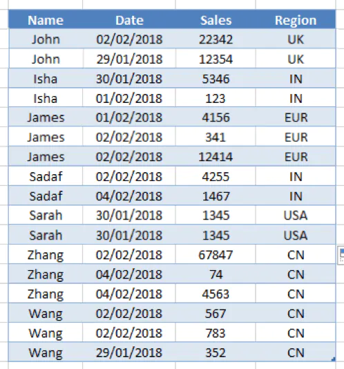
Criteria Range
The criteria range are the rules that will be applied to the data when using the VBA Advanced Filter. You can set one or multiple criteria.
- This can be set up as a range of cells or as a table
- To set up a table, simply select the range of cells including the headers and click Insert → Table
- You can rename your table by clicking anywhere on the new table and editing the text where it says ‘Table1’
- Note: The headers need to match the headers from the database exactly
- You don’t need to have every header – just the ones you want to filter by
-
You can use operators within the cell such as:
- < Less than
- > Greater than
- >= Greater than or equal to
- <= Less than or equal to
- <> Not equal to
For example, <1000 in the cell would return items that are less than 1000
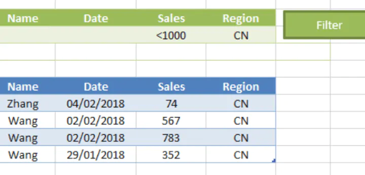
Extract Range
This tool allows you to set an area of data to copy or move. This is particularly useful if, for example, you want to export out a list of contacts or locations. To set this up:
- The same rule applies here as the criteria range; the headers need to be exactly the same
- Note: The headers don’t need to be in the same order and you don’t have to filter all of the columns – just the ones you want to see. For example, if you wanted just a list of names then you would have only the ‘Name’ column on your chosen extract sheet.
Apply the advanced filter
This is to set the area you want to copy the filtered items to.
- Select any cell in the database
- On the Excel Ribbon Data tab, click advanced filtering
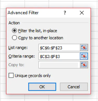
- You can choose to filter in place or to another location, depending on how you want to extract the data
- Set the criteria range
- Note: When copying to another location Excel will clear any data already stored in your extract location when the filter is applied
- Click OK
Filtering unique items
There is an option when filtering to only return unique items. This will return only 1 record that meets each of the criteria you have set. To do this:
-
Simply tick the unique box when filtering
Setting up VBA
Advanced filtering is all well and good, but we have to click ‘advanced filter’ every time we want to filter the list down. This is fine, but it’s not why you came to this article!
First, we need to access the Visual Basic screen in Excel – by default, this is turned off. To turn it on go to:
- File → Options → Ribbon Settings and turn on the Developer tab
- This should turn on an extra tab in Excel so you can create, record and modify VBA code using Macros.
- There are a few kinds of Macros – we will cover:
- Macros that run by clicking on a button
- Macros that run when a cell or range is modified
Button VBA macro
To create a button that triggers a VBA macro we need to create a ‘Module’ within VBA. To do this:
- Navigate to the Developer tab and click on ‘Visual Basic’
- Right-click on ‘Excel Objects Folder’ and click ‘Create New Module’:
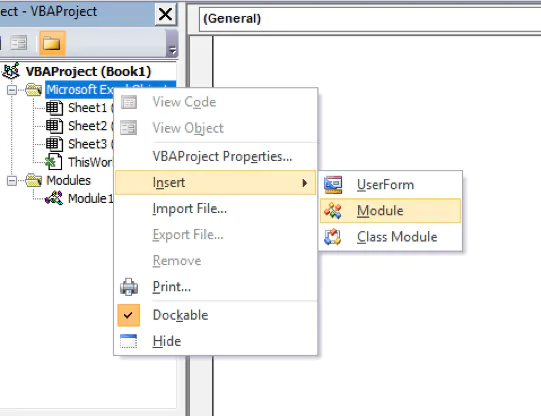
Once you’ve created the new module we can start writing a Macro:
- We always start with Sub NameOfTheSubroutine () and end with End Sub
- We would write our code in-between those lines. For example:
Sub Advanced Filtering ()
End Sub
Here is the start of our VBA code that would go in between the lines above:
- The «Database» would be replaced with the range area of our data
- The «Criteria» would be replaced by our Criteria range
Range("Database").AdvancedFilter _
Action:=xlFilterInPlace, _
CriteriaRange:=Range("Criteria")
VBA Code so far:
Sub Advanced_Filtering()

Range("C6:F23").AdvancedFilter _
Action:=xlFilterInPlace, _
CriteriaRange:=Range("C2:F3")

End Sub
We now need to add a button:
- Insert → Shape → Pick a Shape and draw it onto the sheet. In this case, we’ll use a rectangle.
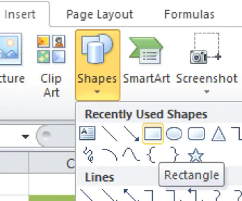
- Assign the Macro you have just created by right-clicking on the shape → Assign Macro. Test it by typing in the criteria range and click the button you’ve just added
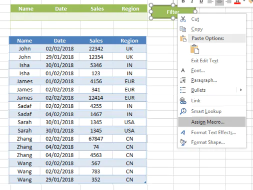
Automatic VBA macro
We’ve just created a button to trigger our macro, but that’s an extra step – we want the list to just filter when we enter something into those cells. To do this we can use Worksheet_Change to trigger the Macro we have just created to run when we update the criteria changes.
-
Right-click on the sheet and click ‘View Code’ – if this doesn’t work you can access via Visual Basic view on the Developer tab. Then double-click on the sheet with your criteria range on it (In this example it’s sheet 1).
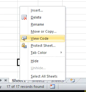
Another way to trigger a VBA Macro is to get Excel to automatically trigger whenever a sheet is updated — In other words when you add, update or change a cell.
This is great, but we don’t want Excel to trigger the code when any cell is updated — We only want to trigger the Macro when a specific range is updated.
- The code below will first check to see if the cells updated are C3 to F3 (our criteria range) and if it’s not it will kill the subroutine (Then Exit Sub).
- If it is within those cells, it triggers our first Macro to run
- This is useful and important as will only allow the code to run when we edit those cells
- If we didn’t have the ‘If Intersect’, it would run every time any cell is changed
Private Sub Worksheet_Change(ByVal Target As Range)

If Intersect(Target, Range("C3:F3")) Is Nothing Or Target.Cells.Count > 1 Then Exit Sub
Call Advanced_Filtering

End Sub
VBA copy to a new location
To alter the VBA to copy to a new location we simply need to change 2 parts of the code:
- We need to change Action:=xlFilterInPlace to Action:=xlFilterCopy
- And add CopyToRange:=Sheets(«SHEET NAME»).Range(«RANGE») to the end
- Here’s what the final code should look like. This will filter the data from Sheet 1 into Sheet 1 in the range A1:D1:
Sub Advanced_Filtering()

CriteriaLastRow = 4 'Last Row you have in the Criteria range

For i = 3 To CriteriaLastRow 'Loops through until the last Row
  RowsCount = Application.WorksheetFunction.CountA(Range("C" & i & ":F" & i))
  If RowsCount = 0 Then CriteriaRowsSet = i - 1 Else CriteriaRowsSet = CriteriaLastRow 'Checks to see if any row returns 0 and sets it to the row above's number
Next i

Range("C6:F23").AdvancedFilter _
Action:=xlFilterInPlace, _
CriteriaRange:=Range("C2:F" & CriteriaRowsSet), _ CopyToRange:=Sheets("Sheet2").Range("A1:D1")

End Sub
What we have gone through so far just covers the basics of filtering, but there is much more filtering is capable of. Let’s take a look at VBA advanced filtering with multiple criteria and wildcards.
Advanced filtering with multiple criteria
Currently, the criteria range can only handle AND statements – meaning it would need to meet all of the criteria to display after filtering. If I wanted to do an OR statement (i.e. I want to show results that are either Wang OR John) then I would need to expand my criteria table:
- First I would expand my row at the bottom to allow for more statements
- Expand both Macros to allow for the extra row
- Note: Make sure when moving or adding new rows that the Macros are still looking at the correct range. Macros are not like formulas that automatically change when you add new rows
- If you do need to add/remove cells then you would need to go back into the VBA code and extend or shorten the range of cells within the code.
If we wanted to remove a column, for example, we would change this code:
Range("C6:F23").AdvancedFilter _
Action:=xlFilterInPlace, _
CriteriaRange:=Range("C2:F" & CriteriaRowsSet), _
CopyToRange:=Sheets("Sheet2").Range("A1:D1")
To this code:
Range("C6:E23").AdvancedFilter _
Action:=xlFilterInPlace, _
CriteriaRange:=Range("C2:E" & CriteriaRowsSet), _
CopyToRange:=Sheets("Sheet2").Range("A1:D1")
Notice I changed both the Filter area and the range Criteria. This is showing me records that are for Wang AND 2/2/2018 OR John: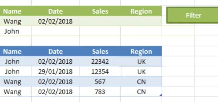
Note: This will not work unless something is contained within both rows or all of the rows if you have more. So we will need to add some code to find which is the bottom row:
- The code below starts off and sets the last row to 4 (meaning the last row number for your criteria)
- It then loops through and checks each row from 3 to your last row and counts how many items are in there
- If it gets right to the bottom and nothing is 0 it sets the criteria range to your full criteria data
- If it returns a 0 on any line it sets the range to the row above it
Sub Advanced_Filtering()

CriteriaLastRow = 4 'Last Row you have in the Criteria range

For i = 3 To CriteriaLastRow 'Loops through until the last Row
  RowsCount = Application.WorksheetFunction.CountA(Range("C" & i & ":F" & i))
  If RowsCount = 0 Then CriteriaRowsSet = i - 1 Else CriteriaRowsSet = CriteriaLastRow 'Checks to see if any row returns 0 and sets it to the row above's number.
Next i

  Range("C6:F23").AdvancedFilter _
  Action:=xlFilterInPlace, _
  CriteriaRange:=Range("C2:F" & CriteriaRowsSet)

End Sub
Advanced filtering with wildcards
Wildcard filtering is where we use a special character to replace a letter to give us similar results.
To use a Wildcard we wouldn’t need to amend any data or VBA code. We would use a symbol within the search criteria.
- The asterisk (*) wildcard character represents any number of characters in that position, including zero characters.
- The question mark (?) wildcard character represents one character in that position.
For example, *ang would return anything that ended with the letters ang:
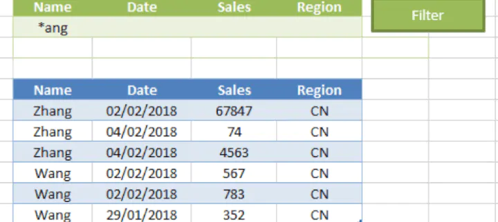
In summary
So, what have we learned?
- That almost any task/function in Excel can be automated using VBA
- How to filter down data more precisely and accurately using VBA
- How to filter down by wildcards
- How to move our filtered data to another location
- How to filter using multiple criteria
- The basics of being able to loop through data and perform a function on each line. This is not just limited to advanced filtering as it can be used with other Excel functions
- The different triggers for VBA in Excel:
- Button – A Macro will run on a click of a button
- Call – A Macro will be ‘called’ (triggered) from another Macro
- Change – A Macro will run when a sheet is updated
This tutorial only covers a small portion of the capability VBA and Macros have in Excel. If you’d like to learn more about creating powerful macros to automate your tasks, check out our Macros and VBA course.
Now that you’ve got filtering down pat, why don’t you try creating your own user defined functions? Learn from the pros with our step-by-step guide on how to build Excel UDFs.
Ready to become a certified Excel ninja?
Take GoSkills’ Macros & VBA course today!
Start free trial
Excel VBA Filter
VBA Filter tool one can use to sort out or fetch the specific data desired. For example, one can use the Autofilter function as a worksheet function. However, this function has other arguments with it which are optional, and the only mandatory argument is the expression that covers the range. For example, worksheets(“Sheet1”).Range(“A1”).Autofilter will apply the filter on the first column.
Filter in VBA works the same way it works in the worksheet. The only thing different is we can automate the routine task of filtering the data through coding.
Table of contents
- Excel VBA Filter
- Examples to Filter Data using VBA
- Example #1 – Apply or Remove Filter to the Data
- Step 1: Supply data range
- Step 2: Then access AutoFilter function
- Step 3: Run the code to enable the filter
- Example #2 – Filter Specific Values
- Step 1: Select Range and Open Autofilter Function
- Step 2: Then Select Field
- Step 3: Now Mention Criteria
- Step 4: And run the code
- Example #3 – Usage of OPERATOR Argument
- Step 1: Select Range and Autofilter Field
- Step 2: Enter Criteria 1 as Math
- Step 3: Use Operator xl
- Step 4: Enter Criteria 2 as Politics
- Example #4 – Filter Numbers with Operator Symbols
- Example #5 – Apply Filter for More Than One Column
- Example #1 – Apply or Remove Filter to the Data
- Things to Remember
- Recommended Articles
- Examples to Filter Data using VBA
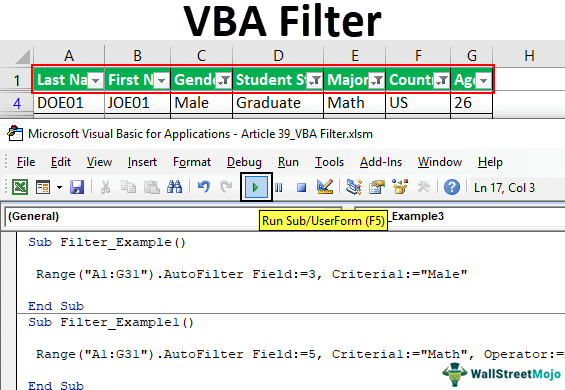
You are free to use this image on your website, templates, etc, Please provide us with an attribution linkArticle Link to be Hyperlinked
For eg:
Source: VBA Filter Data (wallstreetmojo.com)
The AutoFilter is a function that includes many syntax values. Below are the parameters involved in the AutoFilter function.
![]()
- The range is the first thing we need to supply to use the “AutoFilter” option. After that, it is simply for which range of cells we need to apply the filter, for example, Range (“A1:D50”).
- The field is the first argument in the function. Once we select the range of cells through the VBA RANGE objectRange is a property in VBA that helps specify a particular cell, a range of cells, a row, a column, or a three-dimensional range. In the context of the Excel worksheet, the VBA range object includes a single cell or multiple cells spread across various rows and columns.read more, we need to mention for which column of the range we want to apply the filter for.
- Criteria 1 is nothing, but in the selected Field, the value that you want to filter out.
- The operator we may use if we want to use the Criteria 2 argument. In this option, we can use the below options.
xlAnd, xlOr, xlBottom10Items, xlTop10Items, xlTop10Percent, xlBottom10Percent, xlFilterCellColor, xlFilterDynamic, xlFilterFontColor, xlFilterIcon, xlFilterValues - Visible Dropdown displays a filter symbol in the filter applied column. If you want to display it, you can supply the argument as TRUE or else FALSE.
Examples to Filter Data using VBA
You can download this VBA Filter Excel Template here – VBA Filter Excel Template
Example #1 – Apply or Remove Filter to the Data
If you want to apply the filter option to the data, then we can turn it off and on this option. For example, look at the below data image.
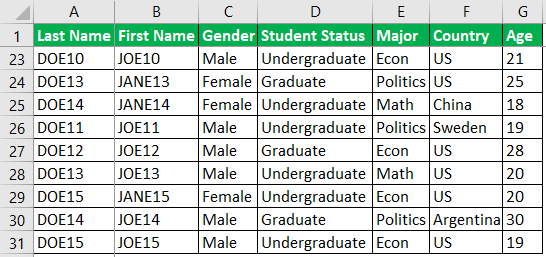
Step 1: Supply data range
To activate the filter option first, we need to supply what is our data range. For example, in the above image, our data is spread from A1 to G31. So, supply this range using a RANGE object.
Code:
Sub Filter_Example()

  Range ("A1:G31")

End Sub

Step 2: Then access AutoFilter function
Now, access the AutoFilter function for this range.
Code:
Sub Filter_Example()

  Range("A1:G31").AutoFilter

End Sub

Step 3: Run the code to enable the filter
That is all. Run this code to enable the AutoFilter.

This code works as a toggle. If the filter is not applied, it will apply. If already applied, then it will be removed.
Example #2 – Filter Specific Values
Now, we will see how to use the parameters of the AutoFilter option. Take the same data as above. For example, we must filter out all “Male” gender names.
Step 1: Select Range and Open Autofilter Function

Step 2: Then Select Field
In the function’s first argument, i.e., Field, we need to mention the column reference we would like to filter out. In this example, we need to filter only “Male” candidates, column “C,” so the column number is 3.

Step 3: Now Mention Criteria
Now for this supplied Field, we need to mention Criteria 1, i.e., what value we need to filter in the Field. We need to filter “Male” from this column.
Code:
Sub Filter_Example()

  Range("A1:G31").AutoFilter Field:=3, Criteria1:="Male"

End Sub

Step 4: And run the code
Ok, that’s all. So this code will filter only “Male” candidates now.

Example #3 – Usage of OPERATOR Argument
When you want to filter out more than one value from the column, we need to use the “Operator” argument. For example, from the column “Major,” we need to filter only “Math & Politics,” then we need to use this argument.
Step 1: Select Range and Autofilter Field
First, supply the Range of cells and fields.
Code:
Sub Filter_Example()

 Range("A1:G31").AutoFilter Field:=5,

End Sub

Step 2: Enter Criteria 1 as Math
For the mentioned field, we need to supply Criteria 1 as “Math.”
Code:
Sub Filter_Example()

 Range("A1:G31").AutoFilter Field:=5, Criteria1:="Math",

End Sub

Step 3: Use Operator xl
Since we need to filter one more value from the same column or field, use the operator symbol as “xlOr.”
Code:
Sub Filter_Example()

  Range("A1:G31").AutoFilter Field:=5, Criteria1:="Math",
  Operator:=xlOr

End Sub

Step 4: Enter Criteria 2 as Politics
And for Criteria 2 argument, mention the value as “Politics.”
Code:
Sub Filter_Example()

 Range("A1:G31").AutoFilter Field:=5, Criteria1:="Math",
 Operator:=xlOr, Criteria2:="Politics"

End Sub

It will filter out both “Math” and “Politics” from column “Major.”

Example #4 – Filter Numbers with Operator Symbols
For example, if you want to filter numbers, we can filter a specific number and numbers above, below, or between specific values and a range of values.
For example, if you want to filter persons aged more than 30, then we can write the code below from the age column.
Code:
Sub Filter_Example()

 Range("A1:G31").AutoFilter Field:=7, Criteria1:=">30"

End Sub
It will filter all the values that are more than 30.
Now, if you want to filter values between 21 and 31, we can use the code below.
Code:
Sub Filter_Example()

 Range("A1:G31").AutoFilter Field:=7, Criteria1:=">21",
 Operator:=xlAnd, Criteria2:="<31"

End Sub
It will filter persons aged between 21 and 30.
Example #5 – Apply Filter for More Than One Column
We need to use a slightly different technique if you want to filter values from more than one column criteria.
If you want to filter “Student Status” as “Graduate” and “Country” as “US,” then first, we need to supply the RANGE of cells under the WITH statement.
Code:
Sub Filter_Example()

  With Range("A1:G31")

  End With

End Sub

Inside the WITH statement, supply the first criteria to be filtered.
Code:
Sub Filter_Example()

 With Range("A1:G31")
  .AutoFilter Field:=4, Criteria1:="Graduate"
 End With

End Sub

Now, in the next line, do the same for “Country” by changing “Field” to six and “Criteria” to “US.”
Code:
Sub Filter_Example()

 With Range("A1:G31")
  .AutoFilter Field:=4, Criteria1:="Graduate"
  .AutoFilter Field:=6, Criteria1:="US"
 End With

End Sub

Now, this will filter “Graduate” only for the country “US.”
Things to Remember
- It will apply the first thing only for the mentioned range of cells filter.
- The field is nothing in which column you want to filter the data.
- If filtering values from more than one column, use the With statement.
Recommended Articles
This article is a guide to VBA Filter. Here we learn how to apply a filter to data, some VBA examples, and download an Excel template. Below are some useful Excel articles related to VBA: –
- VBA AutoFilter
- VBA Do Loop
- How to Enable Solver in VBA?
- Add Filter in Excel
- VBA Paste Values
In this Article
- Advanced Filter Syntax
- Filtering Data In Place
- Resetting the data
- Filtering Unique Values
- Using the CopyTo argument
- Removing Duplicates from the data
This tutorial will explain the how to use the Advanced Filter method in VBA
Advanced Filtering in Excel is very useful when dealing with large quantities of data where you want to apply a variety of filters at the same time. It can also be used to remove duplicates from your data. You need to be familiar with creating an Advanced Filter in Excel before attempting to create an Advanced Filter from within VBA.
Consider the following worksheet.
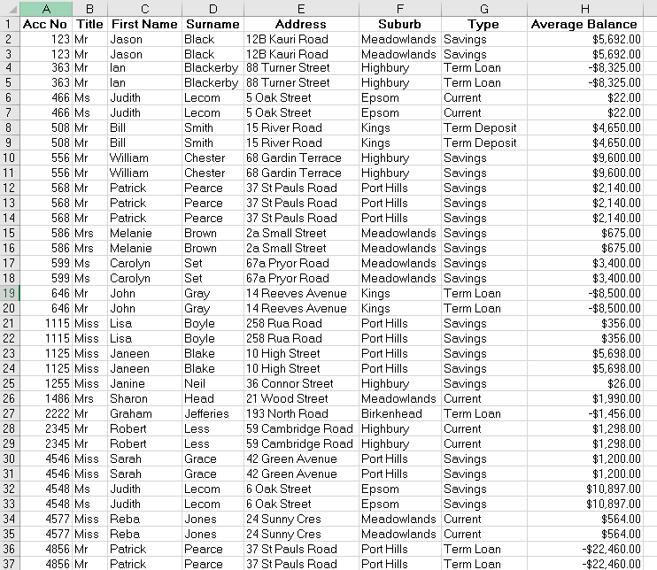
You can see at a glance that there are duplicates that you might wish to remove. The Type of account is a mixture of Saving, Term Loan and Check.
First you need to set up a criteria section for the advanced filter. You can do this in a separate sheet.
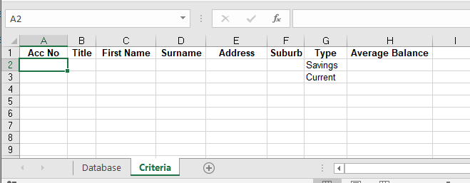
For ease of reference, I have named my data sheet ‘Database’ and my criteria sheet ‘Criteria’.
Advanced Filter Syntax
Expression.AdvancedFilter Action, CriteriaRange, CopyToRange, Unique
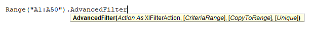
- The Expression represents the range object – and can be set as a Range (eg Range(“A1:A50”) – or the Range can be assigned to a variable and that variable can be used.
- The Action argument is required and will either be xlFilterInPlace or xlFilterCopy
- The Criteria Range argument is where you are getting the Criteria to filter from (our Criteria sheet above). This is optional as you would not need a criteria if you were filtering for unique values for example.
- The CopyToRange argument is where you are going to put your filter results – you can filter in place or you can have your filter result copied to an alternative location. This is also an optional argument.
- The Unique argument is also optional – True is to filter on unique records only, False is to filter on all the records that meet the criteria – if you omit this, the default will be False.
Filtering Data In Place
Using the criteria shown above in the criteria sheet – we want to find all the accounts with a type of ‘Savings’ and ‘Current’. We are filtering in place.
Sub CreateAdvancedFilter()
   Dim rngDatabase As Range
   Dim rngCriteria As Range
'define the database and criteria ranges
   Set rngDatabase = Sheets("Database").Range("A1:H50")
   Set rngCriteria = Sheets("Criteria").Range("A1:H3")
'filter the database using the criteria
   rngDatabase.AdvancedFilter xlFilterInPlace, rngCriteria
End Sub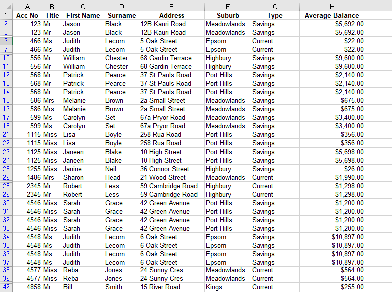
The code will hide the rows that do not meet the criteria.
In the above VBA procedure, we did not include the CopyToRange or Unique arguments.
Resetting the data
Before we run another filter, we have to clear the current one. This will only work if you have filtered your data in place.
Sub ClearFilter()
   On Error Resume Next
'reset the filter to show all the data
   ActiveSheet.ShowAllData
End Sub
Filtering Unique Values
In the procedure below, I have included the Unique argument but omitted the CopyToRange argument. If you leave this argument out, you EITHER have to put a comma as a place holder for the argument
Sub UniqueValuesFilter1()
   Dim rngDatabase As Range
   Dim rngCriteria As Range
'define the database and criteria ranges
   Set rngDatabase = Sheets("Database").Range("A1:H50")
   Set rngCriteria = Sheets("Criteria").Range("A1:H3")
'filter the database using the criteria
   rngDatabase.AdvancedFilter xlFilterInPlace, rngCriteria,,True
End Sub
OR you need to use named arguments as shown below.
Sub UniqueValuesFilter2()
   Dim rngDatabase As Range
   Dim rngCriteria As Range
'define the database and criteria ranges
   Set rngDatabase = Sheets("Database").Range("A1:H50")
   Set rngCriteria = Sheets("Criteria").Range("A1:H3")
'filter the database using the criteria
   rngDatabase.AdvancedFilter Action:=xlFilterInPlace, CriteriaRange:=rngCriteria, Unique:=True
End Sub
Both of the code examples above will run the same filter, as shown below – the data with only unique values.
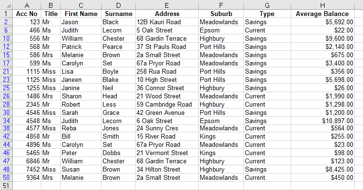
Using the CopyTo argument
Sub CopyToFilter()
   Dim rngDatabase As Range
   Dim rngCriteria As Range
'define the database and criteria ranges
   Set rngDatabase = Sheets("Database").Range("A1:H50")
   Set rngCriteria = Sheets("Criteria").Range("A1:H3")
'copy the filtered data to an alternative location
    rngDatabase.AdvancedFilter Action:=xlFilterCopy, CriteriaRange:=rngCriteria, CopyToRange:=Range("N1:U1"), Unique:=True
End Sub
Note that we could have omitted the names of the arguments in the Advanced Filter line of code, but using named arguments does make the code easier to read and understand.
This line below is identical to the line in the procedure shown above.
rngDatabase.AdvancedFilter xlFilterCopy, rngCriteria, Range("N1:U1"), TrueOnce the code is run, the original data is still shown with the filtered data shown in the destination location specified in the procedure.
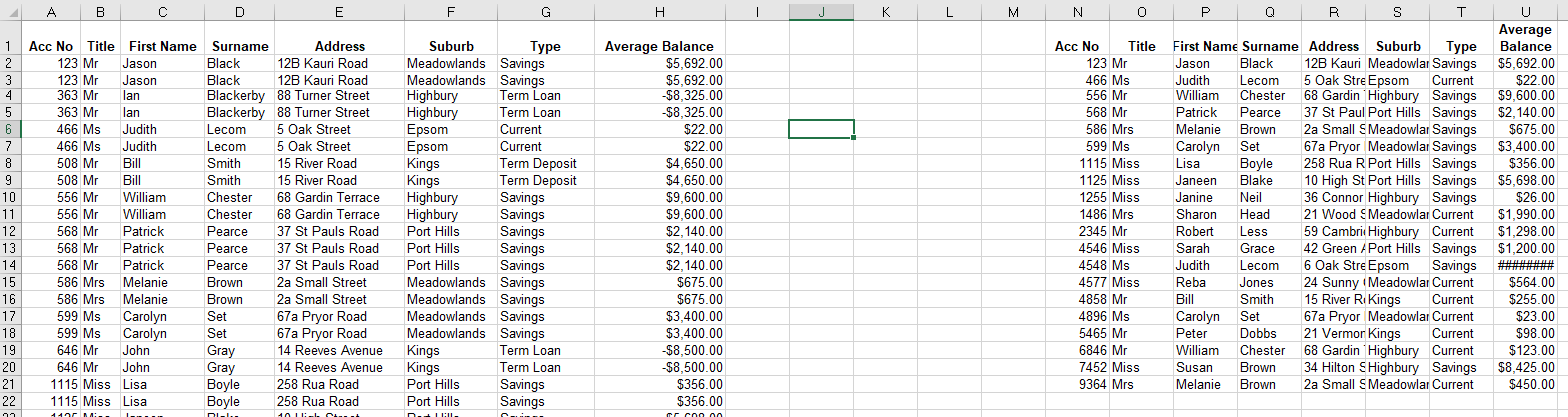
Removing Duplicates from the data
We can remove duplicates from the data by omitting the Criteria argument, and copying the data to a new location.
Sub RemoveDuplicates()
   Dim rngDatabase As Range
'define the database
   Set rngDatabase = Sheets("Database").Range("A1:H50")
'filter the database to a new range with unique set to true
rngDatabase.AdvancedFilter Action:=xlFilterCopy, CopyToRange:=Range("N1:U1"), Unique:=True
End Sub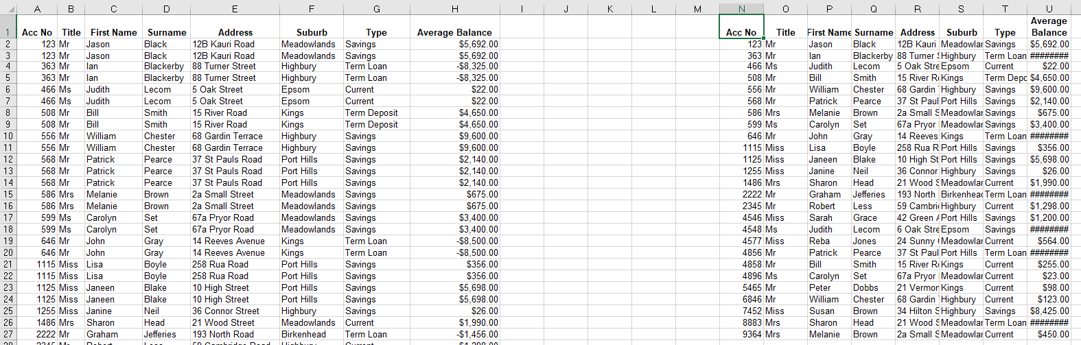
VBA Coding Made Easy
Stop searching for VBA code online. Learn more about AutoMacro — A VBA Code Builder that allows beginners to code procedures from scratch with minimal coding knowledge and with many time-saving features for all users!

Learn More!