Set color to cell in excel - Word и Excel - помощь в работе с программами

You can highlight data in cells by using Fill Color to add or change the background color or pattern of cells. Here’s how:

Select the cells you want to highlight.
Tips:
- To use a different background color for the whole worksheet, click the Select All button. This will hide the gridlines, but you can improve worksheet readability by displaying cell borders around all cells.
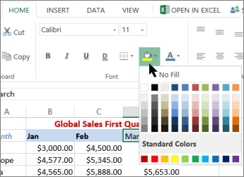
Click Home > the arrow next to Fill Color , or press Alt+H, H.
Under Theme Colors or Standard Colors, pick the color you want.

To use a custom color, click More Colors, and then in the Colors dialog box select the color you want.

Tip: To apply the most recently selected color, you can just click Fill Color . You’ll also find up to 10 most recently selected custom colors under Recent Colors.

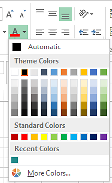
Apply a pattern or fill effects

When you want something more than a just a solid color fill, try applying a pattern or fill effects.

Select the cell or range of cells you want to format.
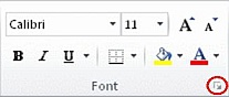
Click Home > Format Cells dialog launcher, or press Ctrl+Shift+F.
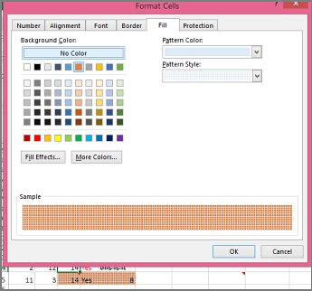
On the Fill tab, under Background Color, pick the color you want.
To use a pattern with two colors, pick a color in the Pattern Color box, and then pick a pattern in the Pattern Style box.

To use a pattern with special effects, click Fill Effects, and then pick the options you want.

Tip: In the Sample box, you can preview the background, pattern, and fill effects you selected.

Remove cell colors, patterns, or fill effects

To remove any background colors, patterns, or fill effects from cells, just select the cells. Then click Home > arrow next to Fill Color, and then pick No Fill.

Print cell colors, patterns, or fill effects in color

If print options are set to Black and white or Draft quality — either on purpose, or because the workbook has large or complex worksheets and charts that caused draft mode to be turned on automatically — cells won’t print in color. Here’s how you can fix that:

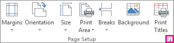
Click Page Layout > Page Setup dialog box launcher.
On the Sheet tab, under Print, uncheck the Black and white and Draft quality check boxes.

Note: If you don’t see colors in your worksheet, it may be that you’re working in high contrast mode. If you don’t see colors when you preview before you print, it may be that you don’t have a color printer selected.

If you’d like to highlight text or numbers to make the data more visible, try either changing the font color or add a background color to the cell or range of cells like this:

Select the cell or range of cells for which you want to add a fill color.
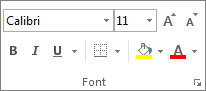
On the Home tab, click Fill Color, and pick the color you want.

Note: Pattern fill effects for background colors are not available for Excel for the web. If you apply any from Excel on your desktop, it won’t appear in the browser.

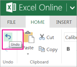
Remove fill color

If you decide that you don’t want the fill color immediately after you added it, just click Undo.

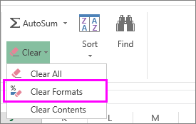
To remove the fill color at a later time, select the cell or cell range you want to change, and click Clear > Clear Formats.

Источник

Заливка ячейки цветом в VBA Excel. Фон ячейки. Свойства .Interior.Color и .Interior.ColorIndex. Цветовая модель RGB. Стандартная палитра. Очистка фона ячейки.

Свойство .Interior.Color объекта Range

Начиная с Excel 2007 основным способом заливки диапазона или отдельной ячейки цветом (зарисовки, добавления, изменения фона) является использование свойства .Interior.Color объекта Range путем присваивания ему значения цвета в виде десятичного числа от 0 до 16777215 (всего 16777216 цветов).

Заливка ячейки цветом в VBA Excel

Пример кода 1:

Sub ColorTest1()

Range(«A1»).Interior.Color = 31569

Range(«A4:D8»).Interior.Color = 4569325

Range(«C12:D17»).Cells(4).Interior.Color = 568569

Cells(3, 6).Interior.Color = 12659

End Sub

Поместите пример кода в свой программный модуль и нажмите кнопку на панели инструментов «Run Sub» или на клавиатуре «F5», курсор должен быть внутри выполняемой программы. На активном листе Excel ячейки и диапазон, выбранные в коде, окрасятся в соответствующие цвета.

Есть один интересный нюанс: если присвоить свойству .Interior.Color отрицательное значение от -16777215 до -1, то цвет будет соответствовать значению, равному сумме максимального значения палитры (16777215) и присвоенного отрицательного значения. Например, заливка всех трех ячеек после выполнения следующего кода будет одинакова:

Sub ColorTest11()

Cells(1, 1).Interior.Color = —12207890

Cells(2, 1).Interior.Color = 16777215 + (—12207890)

Cells(3, 1).Interior.Color = 4569325

End Sub

Проверено в Excel 2016.

Вывод сообщений о числовых значениях цветов

Числовые значения цветов запомнить невозможно, поэтому часто возникает вопрос о том, как узнать числовое значение фона ячейки. Следующий код VBA Excel выводит сообщения о числовых значениях присвоенных ранее цветов.

Пример кода 2:

Sub ColorTest2()

MsgBox Range(«A1»).Interior.Color

MsgBox Range(«A4:D8»).Interior.Color

MsgBox Range(«C12:D17»).Cells(4).Interior.Color

MsgBox Cells(3, 6).Interior.Color

End Sub

Вместо вывода сообщений можно присвоить числовые значения цветов переменным, объявив их как Long.

Использование предопределенных констант

В VBA Excel есть предопределенные константы часто используемых цветов для заливки ячеек:

Предопределенная константа	Наименование цвета
vbBlack	Черный
vbBlue	Голубой
vbCyan	Бирюзовый
vbGreen	Зеленый
vbMagenta	Пурпурный
vbRed	Красный
vbWhite	Белый
vbYellow	Желтый
xlNone	Нет заливки

Присваивается цвет ячейке предопределенной константой в VBA Excel точно так же, как и числовым значением:

Пример кода 3:

Range(«A1»).Interior.Color = vbGreen

Цветовая модель RGB

Цветовая система RGB представляет собой комбинацию различных по интенсивности основных трех цветов: красного, зеленого и синего. Они могут принимать значения от 0 до 255. Если все значения равны 0 — это черный цвет, если все значения равны 255 — это белый цвет.

Выбрать цвет и узнать его значения RGB можно с помощью палитры Excel:

Палитра Excel

Чтобы можно было присвоить ячейке или диапазону цвет с помощью значений RGB, их необходимо перевести в десятичное число, обозначающее цвет. Для этого существует функция VBA Excel, которая так и называется — RGB.

Пример кода 4:

Range(«A1»).Interior.Color = RGB(100, 150, 200)

Список стандартных цветов с RGB-кодами смотрите в статье: HTML. Коды и названия цветов.

Очистка ячейки (диапазона) от заливки

Для очистки ячейки (диапазона) от заливки используется константа xlNone:

Range(«A1»).Interior.Color = xlNone

Свойство .Interior.ColorIndex объекта Range

До появления Excel 2007 существовала только ограниченная палитра для заливки ячеек фоном, состоявшая из 56 цветов, которая сохранилась и в настоящее время. Каждому цвету в этой палитре присвоен индекс от 1 до 56. Присвоить цвет ячейке по индексу или вывести сообщение о нем можно с помощью свойства .Interior.ColorIndex:

Пример кода 5:

Range(«A1»).Interior.ColorIndex = 8

MsgBox Range(«A1»).Interior.ColorIndex

Просмотреть ограниченную палитру для заливки ячеек фоном можно, запустив в VBA Excel простейший макрос:

Пример кода 6:

Sub ColorIndex()

Dim i As Byte

For i = 1 To 56

Cells(i, 1).Interior.ColorIndex = i

End Sub

Номера строк активного листа от 1 до 56 будут соответствовать индексу цвета, а ячейка в первом столбце будет залита соответствующим индексу фоном.

Подробнее о стандартной палитре Excel смотрите в статье: Стандартная палитра из 56 цветов, а также о том, как добавить узор в ячейку.

Источник

Color in Excel (Table of Contents)

Introduction to Color in Excel
Ways to Change Background Color

Introduction to Color in Excel

Colors are generally used to highlight a group of cells in Excel. The excel contains the index of 56 colors. By using conditional formatting, we can put some conditions and apply different colors for different conditions if we want to change the background color of the cell in Excel. We usually select the cells and click the Fill color option; then, the background color will get changed if we want to change the cell’s background colour with the cell automatically.

Ways to Change Background Color

There are two ways to change the background color.

You can download this Color Excel Template here – Color Excel Template

1. Change the color of the cell based on the current value

Here the background color of the cell changes when the cell value in the Excel changes.
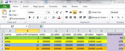
For example, we have taken the following dataset. we want the USD Amount greater than 10,000 as blue color and remaining red color.

Select the range of the cells which we want to change. Then go to the Home tab, go to the styles and select the conditional formatting.

Now click on the new rules.
A dialog appears stating the selection of the row. Select the format of the cells based on the cell value.

Now give the range of values which are greater than 10,000 and select the color as blue color.

Now click on the format option.

A color box appears and makes the Pattern Color as Automatic, so Select color as blue and click on OK.

We can observe that the sample option is blue because we have selected the blue color.

We can observe the selected color in the format option. And click the Ok option.

Now we can use the same procedure for selecting the color for less value. A dialog appears stating the selection of the row. Select the format of the cells based on the cell value. A dialog appears stating the selection of the row. Select the format of the cells based on the cell value. Now give the range of values which are less than 10,000 and select the color as red color.

The color box appears and makes the pattern as automatic and Select color like blue and click OK.
The output will be as follows.

2. Change the background color of special cells

This is another way of color the background of the particular cell. First, go to the home tab, then select the conditional formatting.

Select the new rules.

The formatting dialog box appears to click on the cells which need to format, which is at the end of the dialog box.

Click on the arrow option at the right end.
Write the new formatting rule using the keyword Is Blank condition. This Is Blank is used to highlighting the background cells which are empty.

Click on the Format option. And select the blue color.

Click on the Ok button.

The output will be as follows.

3. Sort the Excel by it Color

Sorting is one of the methods to select a particular color. First, select the cells, right-click on them, select the sort option, and then select the highest value by color.

Click the ok button.
And Filter the color by its color.

sort

And the output will be as follows.

Change the cell color based on the current value.

First, go to the home tab, select the Find and select option, and select the Find option.

find 1

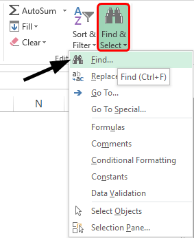
Select the value which we want to select. Click on the Find all option.

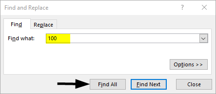
Click on the values range which we want the cells we want to highlight.
Click on the Select by value option. And select the Greater in the list.
Click on the range of the cells we want to highlight. Click on the select option.
Now select the color as blue for the greater value.
And the output will be as follows.

Conditional Formatting in Excel

Conditional formatting is generally used to color data bars and icons in the cells.
To do the conditional formatting in Excel, first, we take the required data set.
Then go to the Home tab and select the conditional formatting option ad put the desired rule which we want to specify, and mention the color which we want to give to the cells of the particular condition.
Then a dialog box appears on the screen then simply gives the values we want a particular condition so that the color will be applied successfully.
Now select the formatting styles from the drop-down. Here we select the color for the condition. Then click the OK. The conditional formatting will be applied to all the cells at a time. This is one way of adding colors to the cells.

Things to Remember About Color in Excel

The colors in excel play a major role in highlighting a particular range of cells.
Here we generally use the two approaches like make the background color cells based on the value, and another way is to change the background of special cells.
The excel contains the index of 56 colors. By using conditional formatting, we can put some conditions and apply different colors for different conditions.
We can also sort the colors based on the colors.
We can highlight the empty cells with the colors.
Through cells, we can highlight the greater values and the lower value with different colors.

How Do You Fill a Cell with Color in Excel?

Open your spreadsheet in Excel.
Select the cell or cells to color.
Click the Home tab at the top of the window.
Click the down arrow to the right of the Fill Color button.
Choose the color to use to fill the cell(s.)

Our article continues below with more information on how to color cells in Excel, as well as pictures of the steps outlined above.

Using formulas like concatenate can greatly improve your working experience with Microsoft Excel, but the formatting of your data can be equally important as the formulas that you use within it.

Learning how to fill a cell with color in Excel is beneficial when you need to visually separate certain types of data in a spreadsheet that you might not otherwise be able to distinguish from one another. The cell fill color makes it easy to identify like types of data that might not be physically located near one another in your worksheet.

Excel spreadsheets can become very difficult to read as they expand to include more rows and columns. This is especially true of spreadsheets that are larger than your screen and require you to scroll in a direction that removes the column or row headings from view.

Last update on 2023-04-13 / Affiliate links / Images from Amazon Product Advertising API
| As an Amazon Associate, I earn from qualifying purchases.

One way to combat this problem with reading Excel data on your screen is to fill a cell with color. If you want to learn how to fill a cell with color in Excel, then maybe you have seen other people create multi-colored spreadsheets that consist of a number of different filled cells that run for the entire length of a row or column.

While initially this might seem like an exercise that is simply meant to make a spreadsheet appear more attractive, it actually serves an important function by letting the document viewer know what row a particular piece of data is contained within.

Our guide on how to expand all rows in Excel can provide you with a simple way to increase the height of your rows in order to show all of the data contained within your cells.

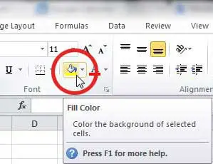
Microsoft Excel 2010 includes a specific tool that you can use to fill a selected cell with a certain color. You can even choose the color that you want to use to fill that cell. That tool is accessed by clicking the Home tab at the top of the Excel window, and is circled in the image below.

use the Excel fill color icon to fill a cell, row or column with color

For example, when I am creating a large spreadsheet, I like to use colors that are distinctly different but are not so distracting that the document becomes hard to read.

If the text in your cells is black, then you will want to avoid using darker fill colors. Sticking to colors like yellow, light green, light blue, and orange will make it very easy for someone to recognize the different cells, but they will not have any difficulty reading the data within them.

This is the most important part because the data is still the reason that the spreadsheet exists in the first place.

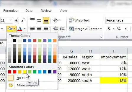
To add color to the background of your cell, you must first click the cell to select it. Click the drop-down arrow to the right of the Fill color icon, then click the color that you want to apply to the selected cell.

The background color will change to the color that you selected. If you want to know how to change fill color in Excel 2010, simply click the cell with the fill color that you want to change, then click the Fill color drop-down arrow and choose a different color.

Now that you know how to color cells in Excel you can use this method to sort and organize your data by simply changing the color of the background in your spreadsheet cells.

If you are not able to change the fill color using this method, then there is some other formatting rule applied to your cell that you need to adjust. Read this article to learn about removing conditional formatting from Excel.

How to Fill a Row With Color in Excel or How to Fill a Column With Color in Excel

The process for applying color to a row or column in Excel is nearly the same as how to apply fill color in Excel to a single cell.

Start by clicking the row or column label (either a letter or number) that you want to apply the fill color to. Once clicked, the entire row should be selected. Click the Fill color icon in the ribbon, then click the color that you want to apply to that row or column. Additionally, if you want to learn how to change the fill color in a row or column in Excel, simply select the filled column or row and use the Fill color icon to select a different color.

By using these methods to apply fill colors to your Excel spreadsheet, you can make it much easier to see which row or column a particular cell is included within. The image below is an example of a spreadsheet that has been completely colored in, which should give you an idea of what you can do with this tool.

Organizing data in this fashion is not particularly necessary when you are dealing with such a small amount of data but, for larger spreadsheets, it can make locating specific types of information much simpler.

Note that using fill colors in this manner is best accomplished when you are done editing your data. The cell fill color won’t stick with the data if you start rearranging rows and columns, so you could wind up with a colorful mess.

Fixing it is as easy as simply re-defining your fill colors, but that can be a pretty big waste of time if you have applied fill color to a lot of your data.

One additional benefit to using fill colors in Excel is the ability to then sort based on those colors. Learn how to sort by fill color in Excel 2010 and take advantage of the formatting that you have applied to your cells.

The next section provides additional information on how to color cells in Excel, such as how to use conditional formatting, and how to apply cell color to multiple cells at the same time.

More Information on How to Format Cells with Cell Color in Microsoft Excel Spreadsheets

Note that you can apply cell colors to one cell, multiple cells, or you could even select the entire sheet by clicking on a single cell then pressing the Ctrl + A keyboard shortcut.

There are some other ways that you can create colored cells in Excel.

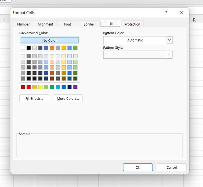
For example, if you select all the cells that you want to color, even if there are multiple cells, then you can right-click on those cells and choose the Format Cells option. This opens the Format Cells dialog box.

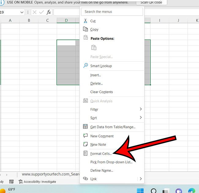
Here you will find a Fill tab at the top of the window that you can use to change the cell background color. You can even click the More Colors button here if you would like to use a color code to modify the color of the cell.

how to color cells in Excel from the Format Cells menu

One other option that you can consider to highlight data with cell colors is to apply conditional formatting. This lets you choose a conditional format based on the cell value so that Excel will format only cells that fit those criteria.

For example, you could choose to format cell values over zero with a green color and make a red cell if it contains a value below zero, or you could apply background colors based on the selected cells containing certain words.

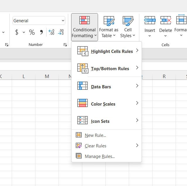
You can find the Conditional Formatting option on the Home tab in the Styles section of the ribbon. Simply click the Conditional Formatting button, choose the parameters, and select format options based on how you want excel to color in your cells.

how to color cells in Excel with conditional formatting

The rules applied during the process of setting up the conditional formatting parameters will apply the cell color based on the options you select.

If none of the color code based options that you see on this dropdown menu offer the solution that you are looking for, then you could click the New rule button and choose your own format.

If you are using Google Sheets and want to be able to color cells, then you are also able to do that. Simply open the spreadsheet in Google Sheets, select the cells that you wish to color, then click the Fill Color button in the toolbar above the spreadsheet. You could also click the Format button at the top of the window and use Conditional formatting or alternating colors there for some more advanced methods of coloring spreadsheet cells.

Additional Sources

Matthew Burleigh has been writing tech tutorials since 2008. His writing has appeared on dozens of different websites and been read over 50 million times.

After receiving his Bachelor’s and Master’s degrees in Computer Science he spent several years working in IT management for small businesses. However, he now works full time writing content online and creating websites.

His main writing topics include iPhones, Microsoft Office, Google Apps, Android, and Photoshop, but he has also written about many other tech topics as well.

Read his full bio here.

Источник

Applies to: Microsoft Excel 365, 2021, 2019, 2016.

In today’s VBA for Excel Automation tutorial we’ll learn about how we can programmatically change the color of a cell based on the cell value.

We can use this technique when developing a dashboard spreadsheet for example.

Step #1: Prepare your spreadsheet

If you are not yet developing on Excel, we’d recommend to look into our introductory guide to Excel Macros. You also need to make sure that the Developer tab is available in your Microsoft Excel Ribbon, as you’ll use it to write some simple code.

Open Microsoft Excel. Note that code provided in this tutorial is expected to function in Excel 2007 and beyond.
In an empty worksheet, add the following table :

Now go ahead and define a named Range by hitting: Formulas>>Define Name

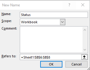
Hit OK

Step #2: Changing cell interior color based on value with Cell.Interior.Color

Hit the Developer entry in the Ribbon.
Hit Visual Basic or Alt+F11 to open your developer VBA editor.
Next highlight the Worksheet in which you would like to run your code. Alternatively, select a module that has your VBA code.
Go ahead and paste this code. In our example we’ll modify the interior color of a range of cells to specific cell RGB values corresponding to the red, yellow and green colors.
Specifically we use the Excel VBA method Cell.Interior.Color and pass the corresponding RGB value or color index.

Sub Color_Cell_Condition()

Dim MyCell As Range
Dim StatValue As String
Dim StatusRange As Range

Set StatusRange = Range("Status")

For Each MyCell In StatusRange

StatValue = MyCell.Value
Select Case StatValue

    Case "Progressing"
    MyCell.Interior.Color = RGB(0, 255, 0)
    
    Case "Pending Feedback"
    MyCell.Interior.Color = RGB(255, 255, 0)
    
    Case "Stuck"
    MyCell.Interior.Color = RGB(255, 0, 0)

End Select

Next MyCell

End Sub

Run your code – either by pressing on F5 or Run>> Run Sub / UserForm.
You’ll notice the status dashboard was filled as shown below:

Save your code and close your VBA editor.

Источник

Apply a pattern or fill effects

Remove cell colors, patterns, or fill effects

Print cell colors, patterns, or fill effects in color

Remove fill color

Свойство .Interior.Color объекта Range

Заливка ячейки цветом в VBA Excel

Вывод сообщений о числовых значениях цветов

Использование предопределенных констант

Цветовая модель RGB

Очистка ячейки (диапазона) от заливки

Свойство .Interior.ColorIndex объекта Range

Introduction to Color in Excel

Ways to Change Background Color

1. Change the color of the cell based on the current value

2. Change the background color of special cells

3. Sort the Excel by it Color

Conditional Formatting in Excel

Things to Remember About Color in Excel

Recommended Articles

How Do You Fill a Cell with Color in Excel?

How to Fill a Row With Color in Excel or How to Fill a Column With Color in Excel

More Information on How to Format Cells with Cell Color in Microsoft Excel Spreadsheets

Additional Sources

Step #1: Prepare your spreadsheet

Step #2: Changing cell interior color based on value with Cell.Interior.Color