
Excel for Microsoft 365 Excel for Microsoft 365 for Mac Excel for the web Excel 2021 Excel 2021 for Mac Excel 2019 Excel 2019 for Mac Excel 2016 Excel 2016 for Mac Excel 2013 Excel 2010 Excel 2007 Excel for Mac 2011 More…Less
Array formulas are powerful formulas that enable you to perform complex calculations that often can’t be done with standard worksheet functions. They are also referred to as «Ctrl-Shift-Enter» or «CSE» formulas, because you need to press Ctrl+Shift+Enter to enter them. You can use array formulas to do the seemingly impossible, such as
-
Count the number of characters in a range of cells.
-
Sum numbers that meet certain conditions, such as the lowest values in a range or numbers that fall between an upper and lower boundary.
-
Sum every nth value in a range of values.
Excel provides two types of array formulas: Array formulas that perform several calculations to generate a single result and array formulas that calculate multiple results. Some worksheet functions return arrays of values, or require an array of values as an argument. For more information, see Guidelines and examples of array formulas.
Note: If you have a current version of Microsoft 365, then you can simply enter the formula in the top-left-cell of the output range, then press ENTER to confirm the formula as a dynamic array formula. Otherwise, the formula must be entered as a legacy array formula by first selecting the output range, entering the formula in the top-left-cell of the output range, and then pressing CTRL+SHIFT+ENTER to confirm it. Excel inserts curly brackets at the beginning and end of the formula for you. For more information on array formulas, see Guidelines and examples of array formulas.
This type of array formula can simplify a worksheet model by replacing several different formulas with a single array formula.
-
Click the cell in which you want to enter the array formula.
-
Enter the formula that you want to use.
Array formulas use standard formula syntax. They all begin with an equal sign (=), and you can use any of the built-in Excel functions in your array formulas.
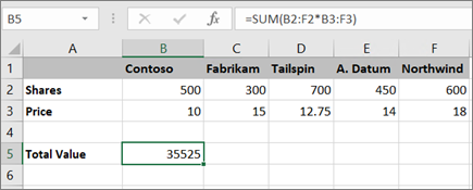
For example, this formula calculates the total value of an array of stock prices and shares, and places the result in the cell next to «Total Value.»

The formula first multiplies the shares (cells B2 – F2) by their prices (cells B3 – F3), and then adds those results to create a grand total of 35,525. This is an example of a single-cell array formula because the formula lives in just one cell.
-
Press Enter (if you have a current Microsoft 365 Subscription); otherwise press Ctrl+Shift+Enter.
When you press Ctrl+Shift+Enter, Excel automatically inserts the formula between { } (a pair of opening and closing braces).
Note: If you have a current version of Microsoft 365, then you can simply enter the formula in the top-left-cell of the output range, then press ENTER to confirm the formula as a dynamic array formula. Otherwise, the formula must be entered as a legacy array formula by first selecting the output range, entering the formula in the top-left-cell of the output range, and then pressing CTRL+SHIFT+ENTER to confirm it. Excel inserts curly brackets at the beginning and end of the formula for you. For more information on array formulas, see Guidelines and examples of array formulas.
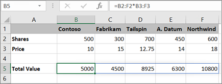
To calculate multiple results by using an array formula, enter the array into a range of cells that has the exact same number of rows and columns that you’ll use in the array arguments.
-
Select the range of cells in which you want to enter the array formula.
-
Enter the formula that you want to use.
Array formulas use standard formula syntax. They all begin with an equal sign (=), and you can use any of the built-in Excel functions in your array formulas.
In the following example, the formula multiples shares by price in each column, and the formula lives in the selected cells in row 5.
-
Press Enter (if you have a current Microsoft 365 Subscription); otherwise press Ctrl+Shift+Enter.
When you press Ctrl+Shift+Enter, Excel automatically inserts the formula between { } (a pair of opening and closing braces).
Note: If you have a current version of Microsoft 365, then you can simply enter the formula in the top-left-cell of the output range, then press ENTER to confirm the formula as a dynamic array formula. Otherwise, the formula must be entered as a legacy array formula by first selecting the output range, entering the formula in the top-left-cell of the output range, and then pressing CTRL+SHIFT+ENTER to confirm it. Excel inserts curly brackets at the beginning and end of the formula for you. For more information on array formulas, see Guidelines and examples of array formulas.
If you need to include new data in your array formula, see Expand an array formula. You can also try:
-
Rules for changing array formulas (they can be finicky)
-
Delete an array formula (you press Ctrl+Shift+Enter there, too)
-
Use array constants in array formulas (they can be handy)
-
Name an array constant (they can make constants easier to use)
If you want to play around with array constants before you try them out with your own data, you can use the sample data here.
The workbook below shows examples of array formulas. To best work with the examples, you should download the workbook to your computer by clicking the Excel icon in the lower-right corner, and then open it in the Excel desktop program.
Copy the table below and paste it into Excel in cell A1. Be sure to select cells E2:E11, enter the formula =C2:C11*D2:D11, and then press Ctrl+Shift+Enter to make it an array formula.
|
Salesperson |
Car Type |
Number Sold |
Unit Price |
Total Sales |
|---|---|---|---|---|
|
Barnhill |
Sedan |
5 |
2200 |
=C2:C11*D2:D11 |
|
Coupe |
4 |
1800 |
||
|
Ingle |
Sedan |
6 |
2300 |
|
|
Coupe |
8 |
1700 |
||
|
Jordan |
Sedan |
3 |
2000 |
|
|
Coupe |
1 |
1600 |
||
|
Pica |
Sedan |
9 |
2150 |
|
|
Coupe |
5 |
1950 |
||
|
Sanchez |
Sedan |
6 |
2250 |
|
|
Coupe |
8 |
2000 |
Create a multi-cell array formula
-
In the sample workbook, select cells E2 through E11. These cells will contain your results.
You always select the cell or cells that will contain your results before you enter the formula.
And by always, we mean 100-percent of the time.
-
Enter this formula. To enter it in a cell, just start typing (press the equal sign) and the formula appears in the last cell you selected. You can also enter the formula in the formula bar:
=C2:C11*D2:D11
-
Press Ctrl+Shift+Enter.
Create a single-cell array formula
-
In the sample workbook, click cell B13.
-
Enter this formula using either method from step 2 above:
=SUM(C2:C11*D2:D11)
-
Press Ctrl+Shift+Enter.
The formula multiplies the values in the cell ranges C2:C11 and D2:D11, then adds the results to calculate a grand total.
In Excel for the web, you can view array formulas if the workbook you open already has them. But you won’t be able to create an array formula in this version of Excel by pressing Ctrl+Shift+Enter, which inserts the formula between a pair of opening and closing braces({ }). Manually entering these braces won’t turn the formula into an array formula either.
If you have the Excel desktop application, you can use the Open in Excel button to open the workbook and create an array formula.
Need more help?
You can always ask an expert in the Excel Tech Community or get support in the Answers community.
Need more help?
Want more options?
Explore subscription benefits, browse training courses, learn how to secure your device, and more.
Communities help you ask and answer questions, give feedback, and hear from experts with rich knowledge.
#Руководства
- 25 июл 2022
-
0
Как с помощью массивов ускорить расчёты в таблицах с тысячами значений? Как поменять местами столбцы и строки? Разбираемся на примерах.
Иллюстрация: Meery Mary для Skillbox Media

Рассказывает просто о сложных вещах из мира бизнеса и управления. До редактуры — пять лет в банке и три — в оценке имущества. Разбирается в Excel, финансах и корпоративной жизни.
Часто новичкам в Excel кажется, что массивы — это высший пилотаж в работе с таблицами. На деле всё гораздо проще.
Массивы в Excel — это данные из двух и более смежных ячеек таблицы, которые используют в расчётах как единую группу, одновременно. Массивом может быть одна строка или столбец, несколько строк или столбцов и даже целые таблицы.
Операции с массивами — не основная функциональность Excel, но они делают работу с большими диапазонами значений удобнее и быстрее. С помощью массивов можно проводить расчёты не поочерёдно с каждой ячейкой диапазона, а со всем диапазоном одновременно. Или создать формулу, которая выполнит сразу несколько действий с любым количеством ячеек.
В статье разберёмся:
- какие виды массивов есть в Excel;
- что такое формула массива и как она работает.
Подробно покажем на примерах, как выполнить четыре базовые операции с помощью формул массивов и операторов Excel:
- построчно перемножить значения двух столбцов;
- умножить одно значение сразу на весь столбец;
- выполнить два действия одной формулой;
- поменять местами положение столбцов и строк таблицы.
В конце расскажем, как создать формулу массива в «Google Таблицах».
Массивы в Excel бывают одномерными и двумерными.
В одномерных массивах все данные расположены в одной строке или в одном столбце. В зависимости от этого их делят на горизонтальные и вертикальные.
Скриншот: Excel / Skillbox Media
Скриншот: Excel / Skillbox Media
В двумерных массивах данные расположены сразу в нескольких столбцах и строках. Такие массивы могут образовывать целые таблицы, а иногда занимают даже несколько листов.
Скриншот: Excel / Skillbox Media
Работа с массивами в Excel похожа на стандартную работу с одиночными ячейками. Отличие в том, что расчёты и операции проводят одновременно для всех значений диапазонов, а не для одного. Для этого используют формулы массивов.
Формула массива — формула, где в качестве входящих параметров используют диапазоны значений, а не одиночные ячейки. Диапазоны значений обозначаются через двоеточие :. Например, A1:A10 или А1:В10.
С формулами массива можно выполнить несколько математических действий одновременно. Например, чтобы перемножить значения двух столбцов и затем суммировать полученные числа, понадобится одна формула массива и одно действие.
В целом формулы массивов работают так же, как и обычные формулы. В них можно использовать любые математические действия.
Формулы массивов можно использовать как для одной ячейки, так и для нескольких одновременно. Например, можно посчитать в одной ячейке сумму значений из нескольких столбцов. Такая формула массива называется одноячеечной. Или можно перемножить значения двух столбцов построчно, а результат вывести в третий. Формула массива будет называться многоячеечной.
В следующих разделах покажем четыре примера, как создавать и использовать формулы массивов.
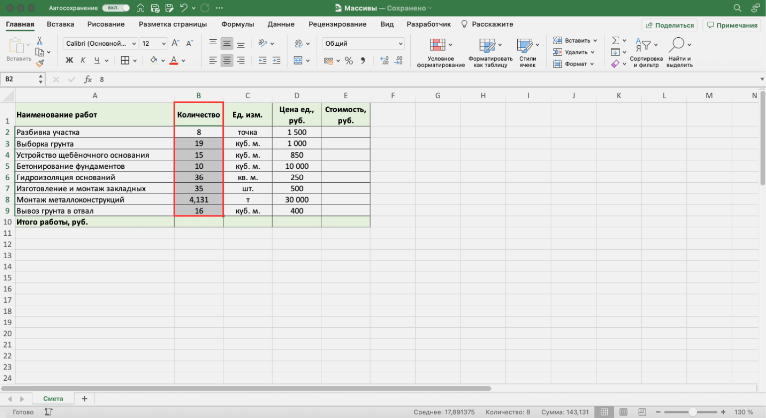
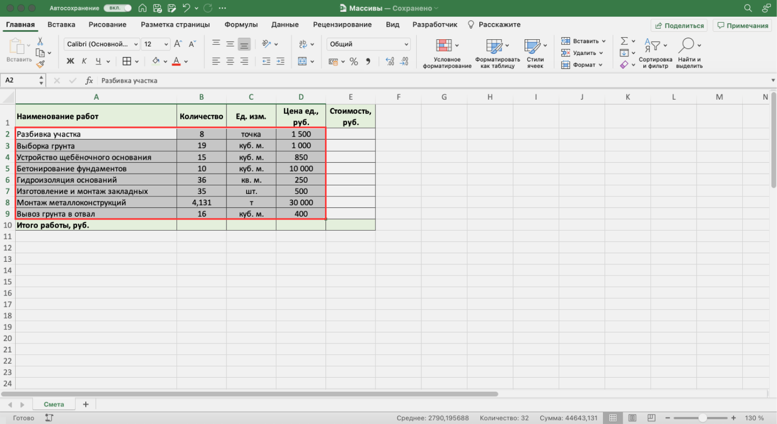
Допустим, нужно рассчитать смету устройства фундаментов. У нас есть перечень необходимых работ, их объёмы и цена единиц измерения объёмов.
Скриншот: Excel / Skillbox Media
Определим стоимость каждой работы.
Можно пойти классическим путём — перемножить первые ячейки столбцов «Количество» и «Цена ед., руб.», а затем растянуть результат вниз на все остальные виды работ. Но если видов будет несколько сотен или тысяч, этот вариант может быть неудобен.
Формула массивов выведет результаты одновременно для всего диапазона — никаких дополнительных действий выполнять не потребуется. Рассмотрим, как это сделать.
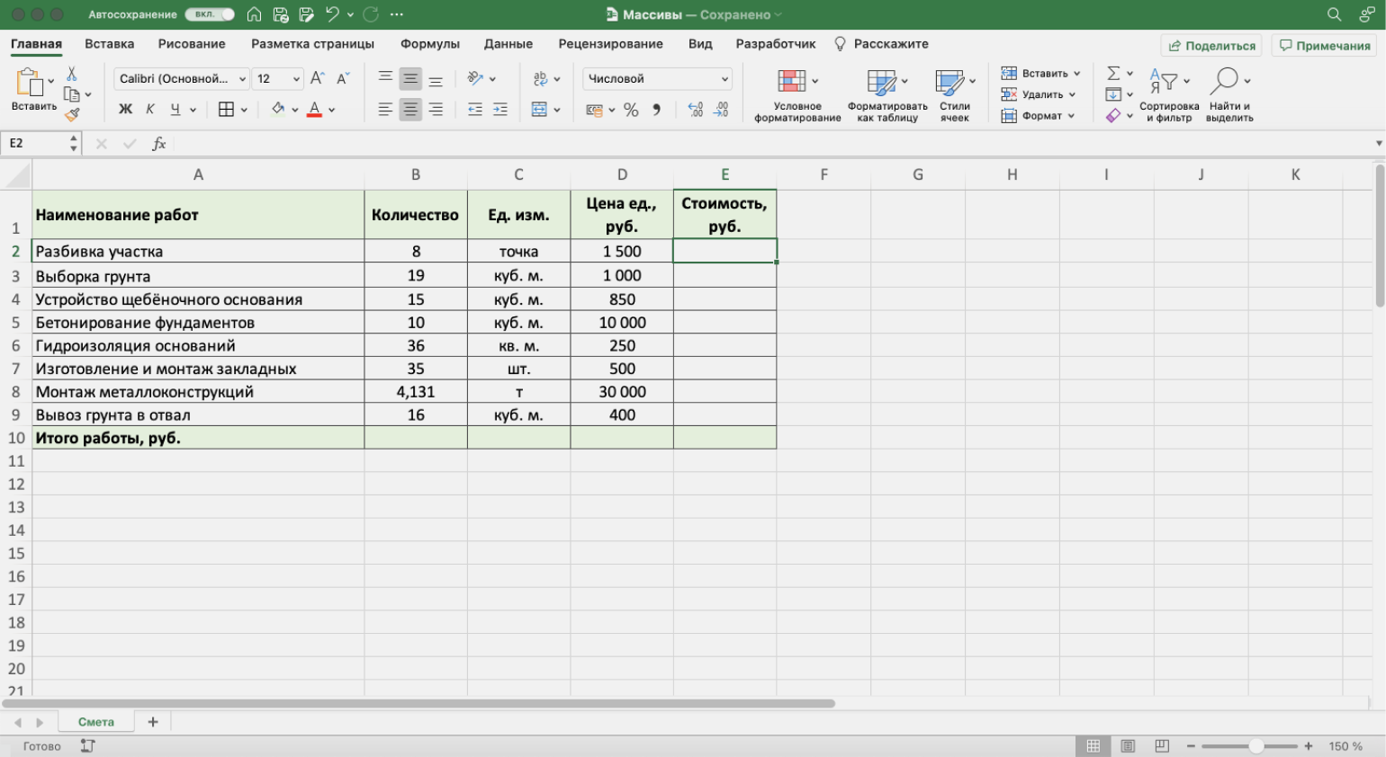
Шаг 1. Выделяем столбец, в котором хотим получить результат расчёта, — в нашем случае это диапазон E2:E9. В строке ссылок вводим знак равенства.
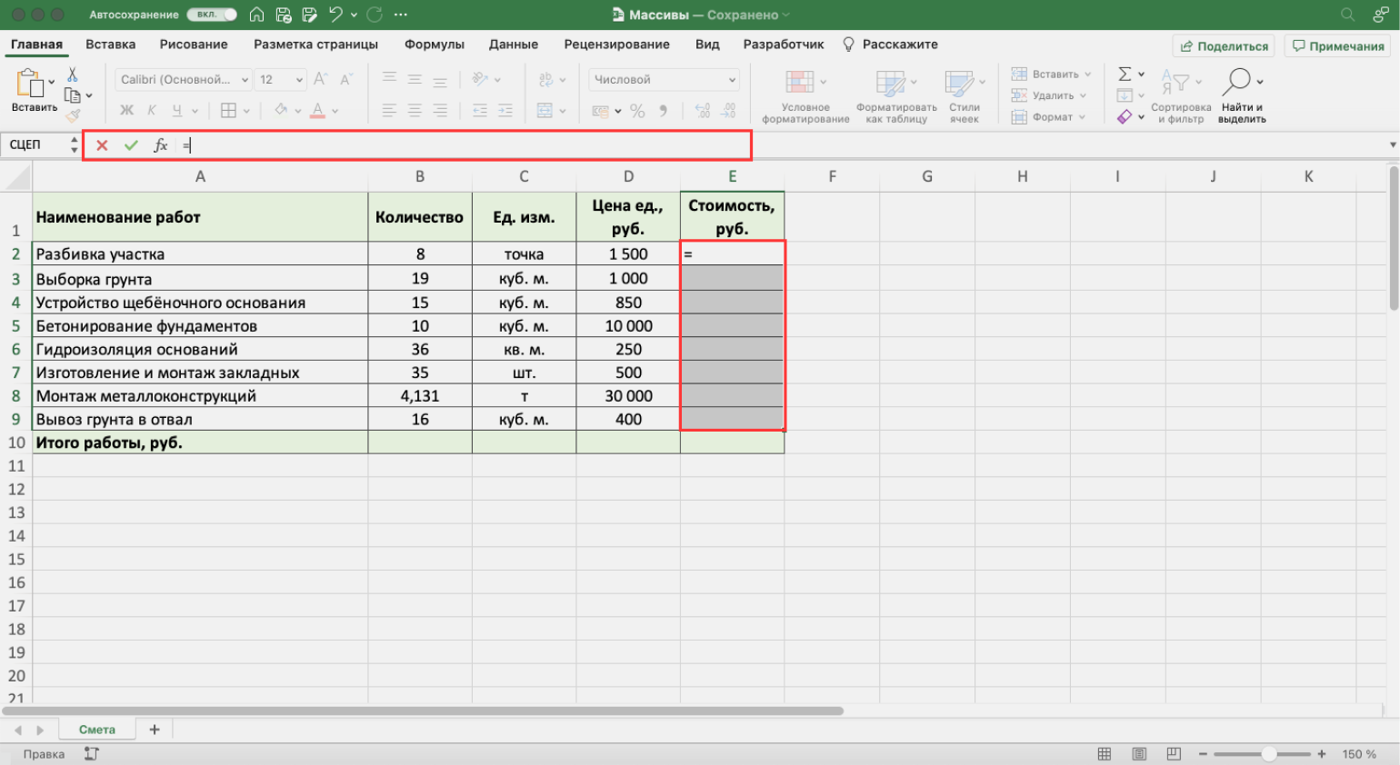
Скриншот: Excel / Skillbox Media
Шаг 2. Выделяем первый массив, который участвует в расчётах, — все значения столбца «Количество». Одновременно с этим в строке ссылок появляется выбранный диапазон: B2:B9.
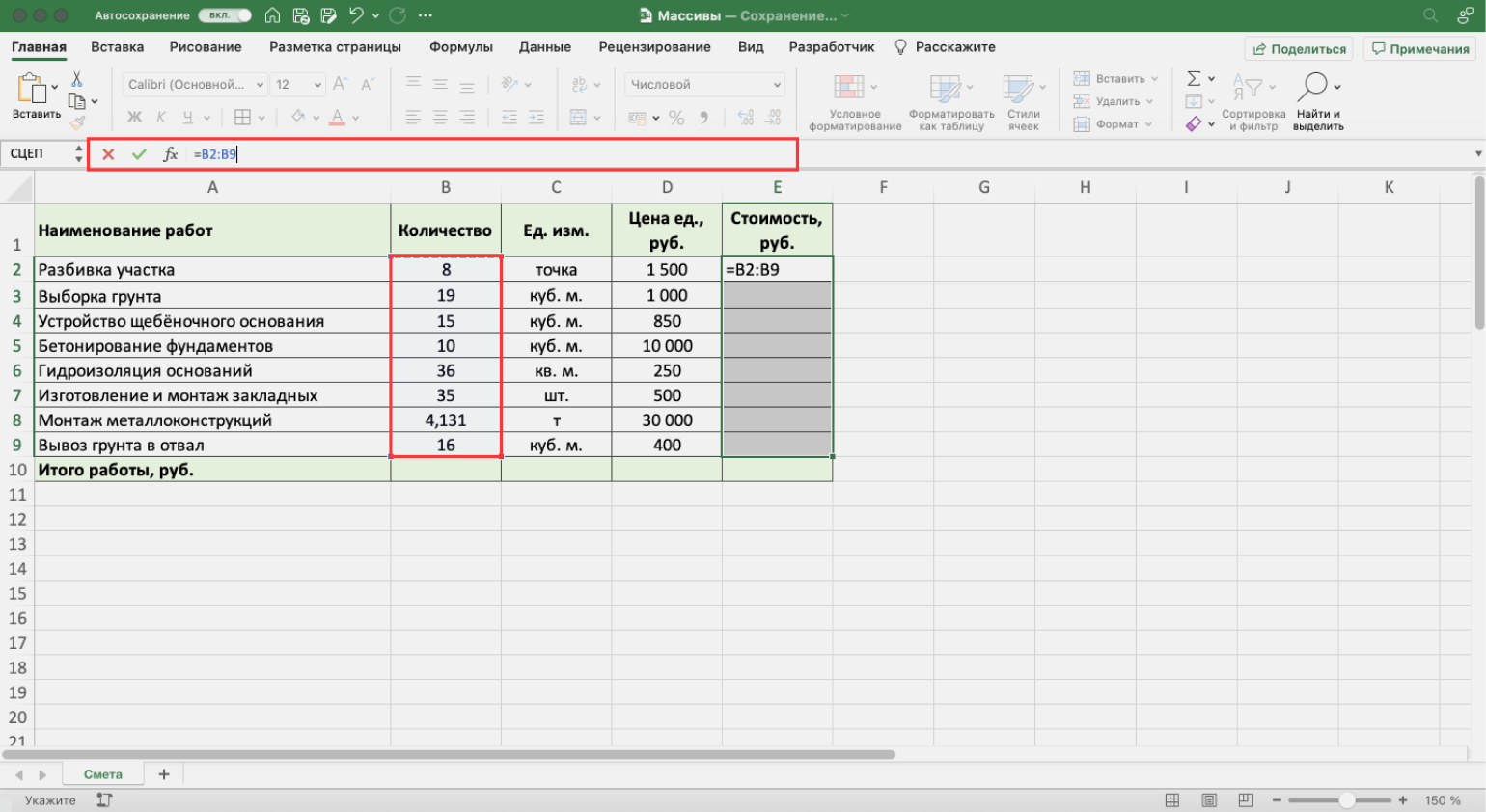
Скриншот: Excel / Skillbox Media
Шаг 3. Ставим знак умножения в строке ссылок и выбираем второй массив — все значения столбца «Цена ед., руб.».
Строка ссылок принимает вид: fx=B2:B9*D2:D9. Это значит, что значения первого массива должны умножиться на значения второго массива.
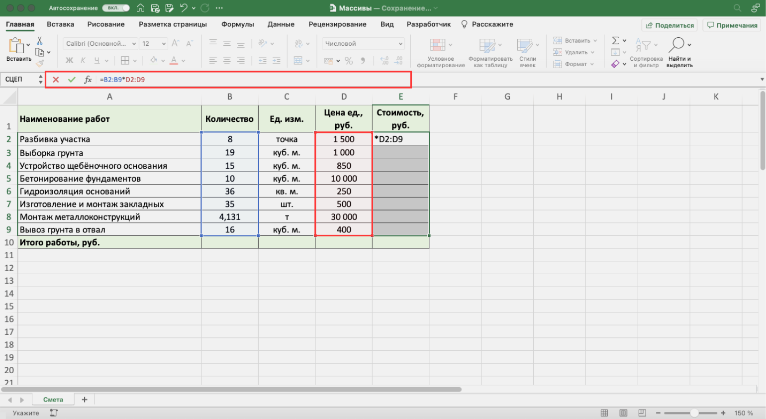
Скриншот: Excel / Skillbox Media
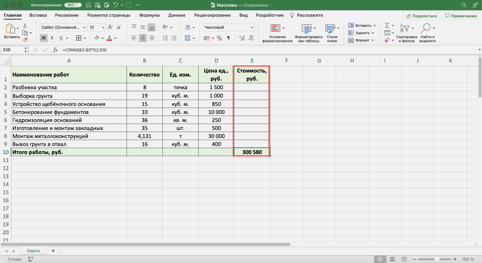
Шаг 4. Нажимаем Enter — в столбце «Стоимость, руб.» появляется результат расчёта. Так, в один клик, формула сработала сразу для всех строк.
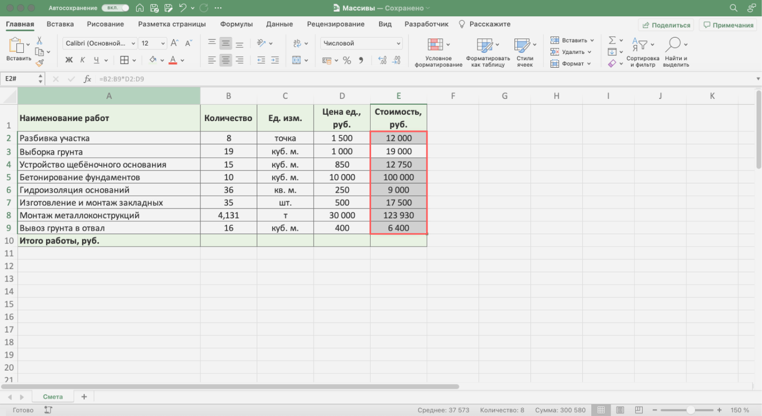
Скриншот: Excel / Skillbox Media
По такому же принципу можно проводить разные арифметические вычисления для одного массива.
Допустим, для нашей сметы нужно рассчитать дополнительные расходы, составляющие долю в общей стоимости работ.
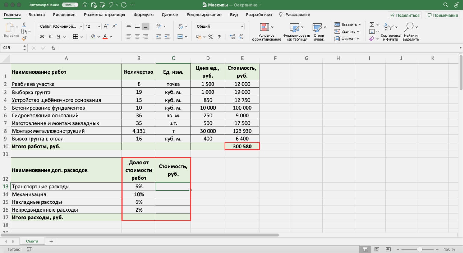
Скриншот: Excel / Skillbox Media
Как и в первом случае, можно перемножить первую ячейку столбца «Доля от стоимости работ» и ячейку с общей стоимостью работ. Затем растянуть результат вниз на все остальные расходы. А можно, для удобства и ускорения процесса, воспользоваться формулой массивов. Она позволит одним действием посчитать сумму всех расходов.
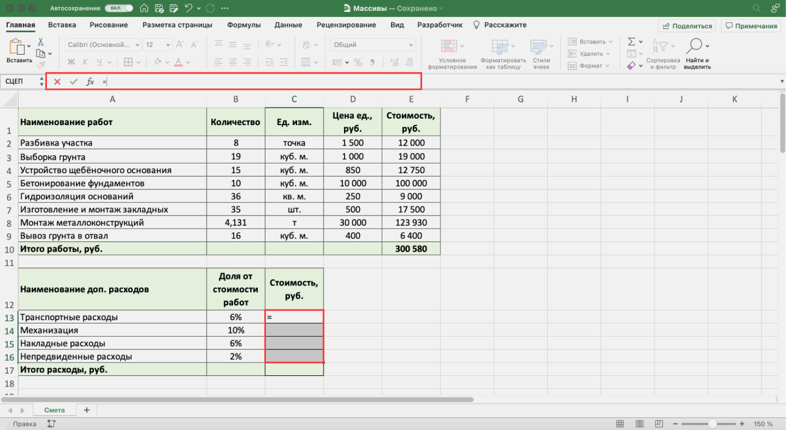
Шаг 1. Выделяем столбец для результата расчёта: С13:С16. В строке ссылок вводим знак равенства.

Скриншот: Excel / Skillbox Media
Шаг 2. Выделяем массив, который участвует в расчётах, — все значения столбца «Доля от стоимости работ». В формуле строки ссылок появляется выбранный диапазон: B13:B16. Добавляем к нему знак умножения и выбираем ячейку с общей стоимостью работ: E10.
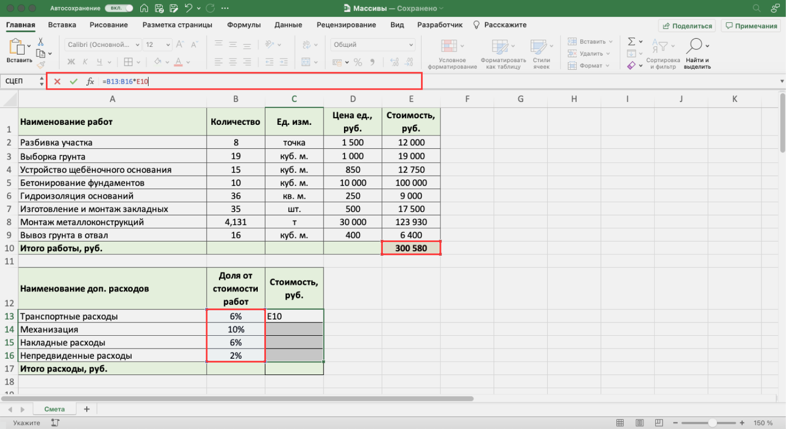
Скриншот: Excel / Skillbox Media
Шаг 3. Нажимаем Enter. Во всём столбце «Стоимость, руб.» появляются результаты расчётов.
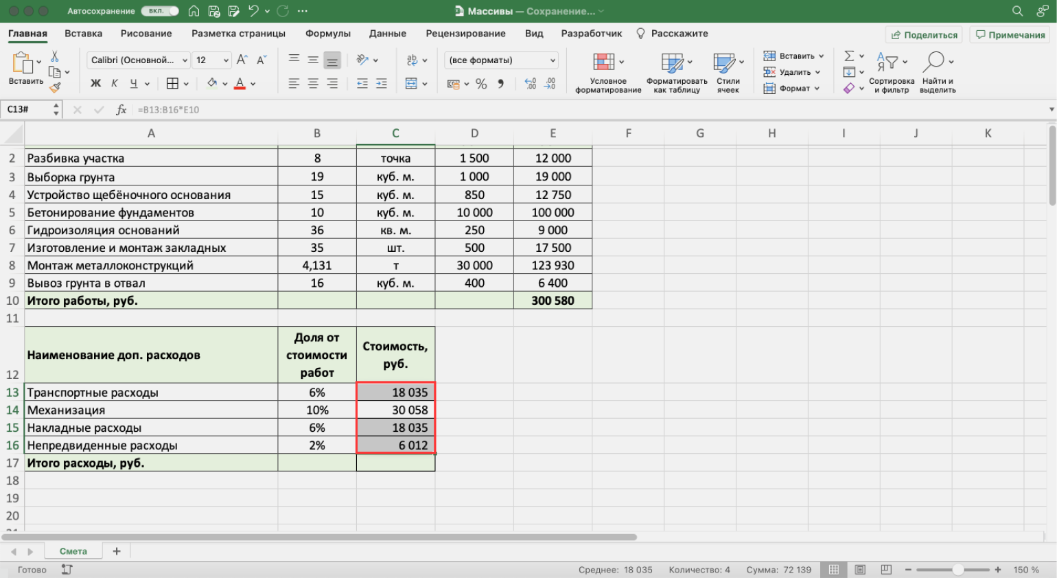
Скриншот: Excel / Skillbox Media
Вернёмся к нашему первому примеру со сметой. Там мы рассчитывали стоимость каждой работы отдельно. Общую стоимость работ в этом случае было проще определить путём сложения всех полученных значений.
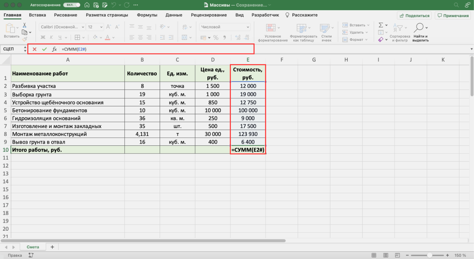
Скриншот: Excel / Skillbox Media
Предположим, нам нужно получить общую стоимость устройства фундаментов одним действием, а стоимость каждой работы отдельно при этом не важна.
Для этого воспользуемся формулой массивов и оператором СУММ. Они выполнят одновременно два математических действия: перемножат столбцы и суммируют полученные результаты.
Шаг 1. Выделяем ячейку, в которой хотим получить результат расчёта. В строке ссылок вводим знак равенства и оператор СУММ и открываем скобку.
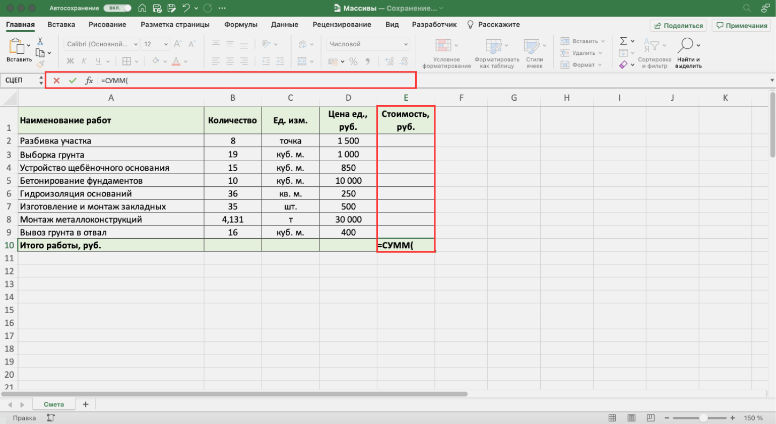
Скриншот: Excel / Skillbox Media
Шаг 2. По аналогии с алгоритмом из предыдущего раздела, выделяем первый массив — значения столбца «Количество» и второй массив — значения столбца «Цена ед., руб.». Ставим между ними знак умножения и закрываем скобку.
Строка ссылок принимает вид: fx=СУММ(B2:B9*D2:D9). Это значит, что значения первого массива должны перемножиться со значениями второго массива, а все полученные результаты — суммироваться.
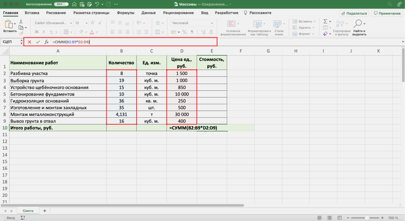
Скриншот: Excel / Skillbox Media
Шаг 3. Нажимаем Enter. В выбранной ячейке появляется результат расчёта. Формула рассчитала одновременно два действия: перемножила значения ячеек двух массивов и суммировала полученные результаты.
Скриншот: Excel / Skillbox Media
По такой же схеме в формулах массивов можно использовать и другие функции Excel. Отличие от их классического применения будет в том, что аргументами будут не отдельные ячейки, а массивы таких ячеек.
Иногда при работе в Excel нужно поменять положение столбцов или строк — транспортировать их. Например, перевести шапку таблицы из горизонтального положения в вертикальное. Делать это вручную долго — особенно, когда ячеек очень много. Ускорить процесс помогут массивы и оператор ТРАНСП:
Шаг 1. Выделяем ячейку, в которой хотим получить результат операции. В строке ссылок вводим знак равенства и оператор ТРАНСП и открываем скобку.
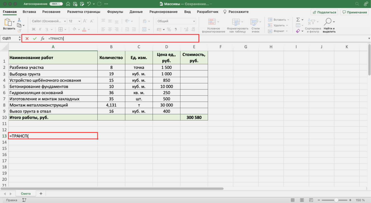
Скриншот: Excel / Skillbox Media
Шаг 2. Выделяем шапку таблицы и закрываем скобку. Строка ссылок принимает вид: fx=ТРАНСП(A1:E1).
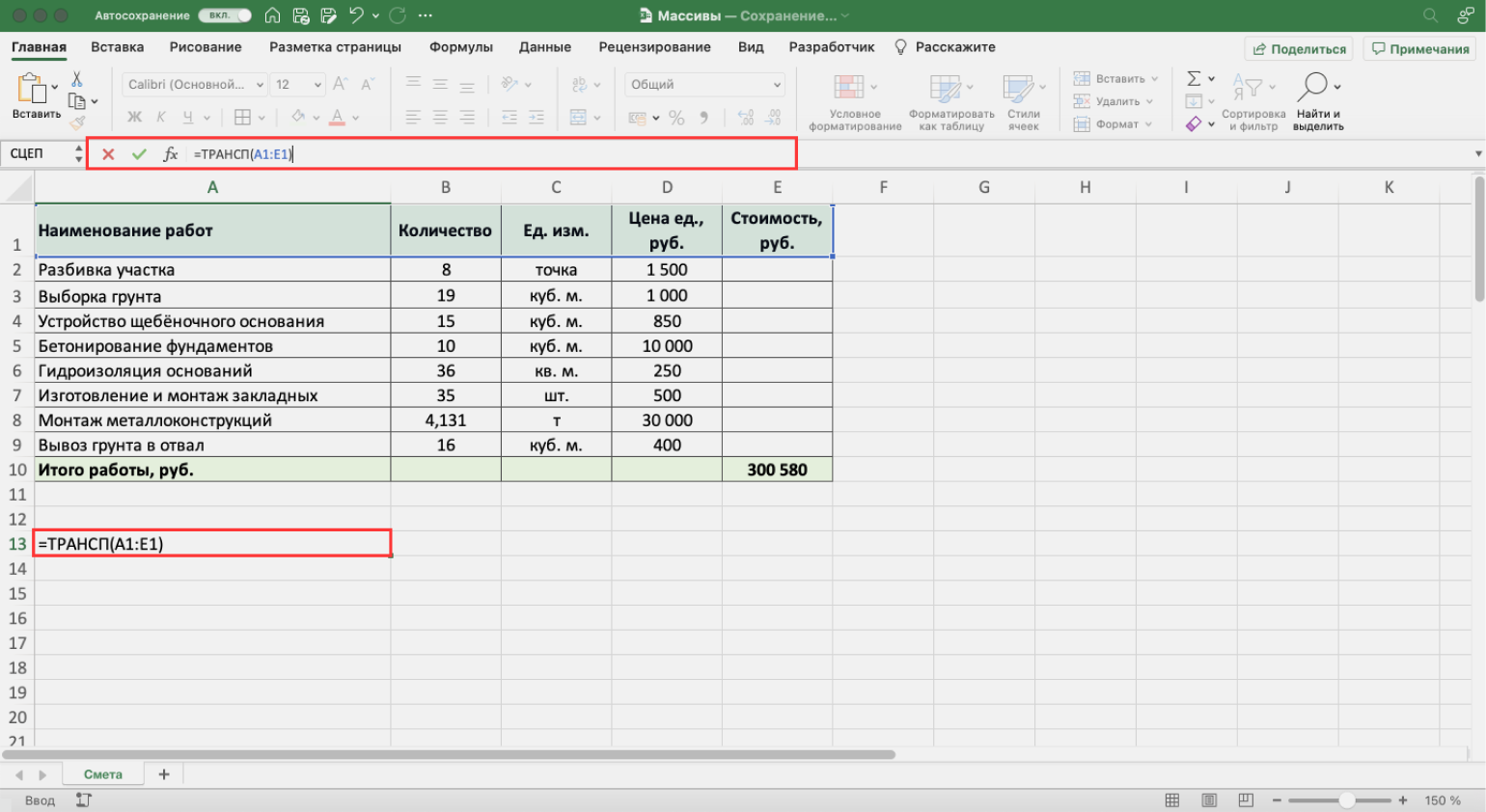
Скриншот: Excel / Skillbox Media
Шаг 3. Нажимаем Enter — функция меняет положение шапки таблицы на вертикальное.
Скриншот: Excel / Skillbox Media
Как создать формулу массива в «Google Таблицах»? Всё точно так же, как в Excel, но нужно добавить оператор ARRAYFORMULA. Его ставят перед всей формулой массива в строке ссылок. Например, если вы хотите перемножить данные в двух столбцах, формула в готовом виде будет выглядеть так:
fx=ARRAYFORMULA(B2:B9*D2:D9).
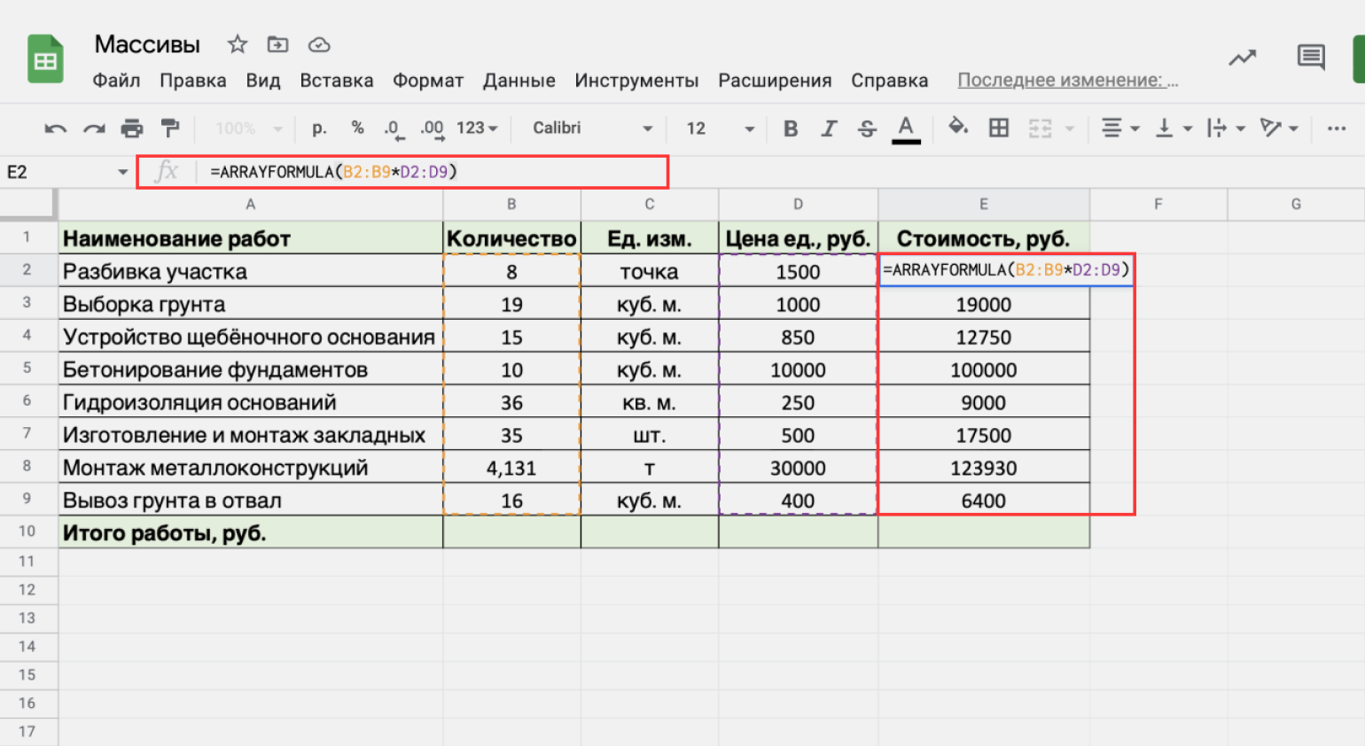
Скриншот: Google Таблицы / Skillbox Media
Другие материалы Skillbox Media по Excel
- Как сделать сводные таблицы в Excel — детальная инструкция со скриншотами
- Руководство: как сделать ВПР в Excel и перенести данные из одной таблицы в другую
- Руководство по макросам для новичков — для чего нужны и как их сделать
- Инструкция: как закреплять строки и столбцы в Excel
- Руководство по созданию выпадающих списков в Excel — как упростить заполнение таблицы повторяющимися данными

Научитесь: Excel + Google Таблицы с нуля до PRO
Узнать больше
The array of Excel functions allows you to solve complex tasks in automatically at the same time. We cannot complete the same tasks through the usual functions.
In fact, this is a group of functions that simultaneously process a group of data and immediately produce a result. Let’s consider in detail work with arrays of functions in Excel.
Types of Excel functions
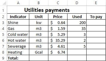
Array is a data grouped together. In this case, the group is an array of functions in Excel. Any table that we compose and fill in Excel can be called an array. Example:
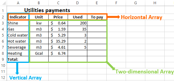
Depending on the location of the elements, the arrays are distinguished:
- One-dimensional (data is in ONE line or in ONE column);
- Two-dimensional (SEVERAL lines and columns, matrix).
One-dimensional arrays are:
- Horizontal (data in a row);
- Vertical (data in a column).
Note. Two-dimensional Excel arrays can take several sheets at once (these are hundreds and thousands of data).
Array formula allows you to process data from this array. It can return one value or result in an array (set) of values.
With the help of array formulas it is real to:
- Count the number of characters in a certain range;
- Summarize only those numbers that correspond to the given condition;
- Summarize all n values in a certain range.
When we use array formulas, Excel takes into account the range of values not as individual cells, but as a single data block.
Array formulas syntax
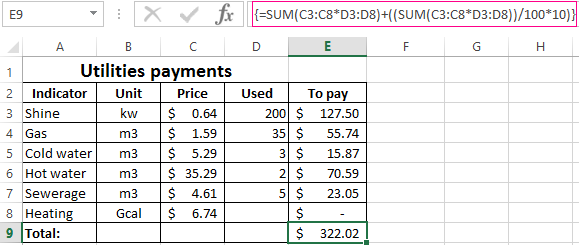
We use the formula of an array with a range of cells and with a separate cell. In the first case, we find the subtotals for the «To pay» «» column. In the second — the total amount of utility payments.
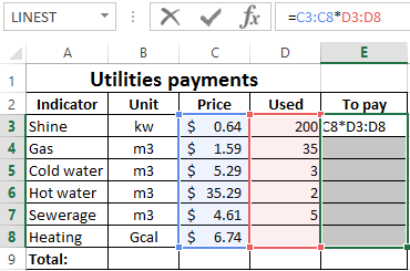
- We select the range E3: E8.
- Enter the following formula in the formula row: = C3: C8 * D3: D8.
- Press the keys simultaneously: Ctrl + Shift + Enter. The subtotals are calculated:
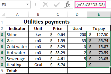
The formula after pressing Ctrl + Shift + Enter was in curly brackets. It was automatically inserted into each cell of the selected range.
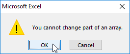
If you try to change the data in any cell in the «To pay» column, nothing happens. The formula in the array protects range values from changes. A corresponding entry appears on the screen:
Consider other examples of using the functions of an Excel array — calculate the total amount of utility payments using a single formula.
- Select the cell E9 (opposite the «Total»).
- We introduce a formula of the form:
- Press the key combination: Ctrl + Shift + Enter. Result:
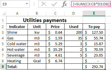
The formula of the array in this case replaced two simple formulas. This is a shortened version, which contains all the necessary information for solving a complex problem.
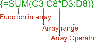
Arguments for a function are one-dimensional arrays. The formula looks at each of them individually, performs user-defined operations, and generates a single result.
Consider the syntax:
Working functions with Excel array
Let’s guess that it is planned to increase utility payments in 10% the next month. If we introduce the usual formula for the total is =SUM((C3:C8*D3:D8)+10%), then we are unlikely to get the expected result. We need each argument to increase in 10%. For the program to understand this, we use the function as an array.
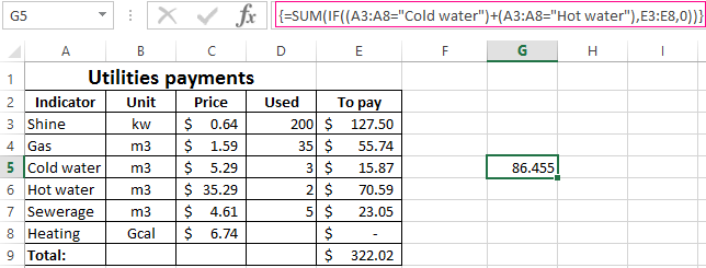
- Let’s have a look how the «И» «AND» operator works in the array function. We need to find out how much we pay for the water, hot and cold. Function:
The total is 86.46$.
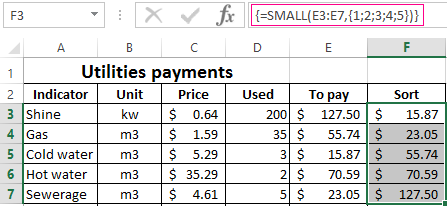
- The Sort functions in the array formula. Sort the amounts to be paid in ascending order. For the sorted data list, create a range. Let’s select it (F3:F7). In the formula bar, we enter
Press Ctrl + Shift + Enter.
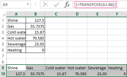
- The transported matrix. There is a special Excel function for working with two-dimensional arrays. The «ТРАНСП» function returns several values at once. It converts a horizontal matrix to a vertical matrix and vice versa. Select the range of cells where the number of rows equals to the number of columns in the table with the original data. And the number of columns equals to the number of rows in the source array. Select range A9:F10. We introduce the formula:
Press Ctrl + Shift + Enter. This results in an «inverted» data set.
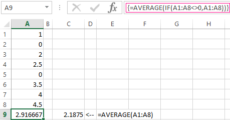
- Search for the average without taking into account zeros. If we use the standard «AVERAGE» function, we get «0» as a result. And it will be correct. Therefore, we insert an additional condition into the formula:
We get:
A common mistake when working with arrays of functions is NOT to press the code combination «Ctrl + Shift + Enter» (never forget this key combination). This is the most important thing to remember when processing large amounts of information. Correctly entered function performs the most complicated tasks.
Download array formula examples
Array formulas are very useful and powerful formulas used to perform some of the very complex calculations in Excel. It is also known as the CSE formula. We need to press “CTRL + SHIFT + ENTER” together to execute array formulas instead of pressing enter. There are two types of array formulas: one that gives us a single result and another that provides multiple results.
For example, suppose you have the data set showing the production and cost for the four products, and you need to calculate the total cost of all the products. We could do this by simply adding formula in the column that multiplies the production and costs of the products and then adding a sum at the bottom of the column. However, the array formulas avoid these steps and provide an answer with a single formula.
Arrays in excelA VBA array in excel is a storage unit or a variable which can store multiple data values. These values must necessarily be of the same data type. This implies that the related values are grouped together to be stored in an array variable.read more can be termed array formulas in Excel. Array in Excel is a powerful formula that enables us to perform complex calculations.
What is an Array? An array is a set of values or variables in a data set like {a,b,c,d} is an array that has values from “a” to “d.” Similarly, in an Excel array is a range of cells of values,

In the above screenshot, cells from B2 to cell G2 are an array or range of cells.
These are also known as “CSE formulas” or “Control Shift Enter Formulas.” For example, for creating an array formula in Excel, we must press “Ctrl + Shift + Enter.”
In Excel, we have two types of array formulas:
- One, which gives us a single result.
- Another which gives us more than one result.
We will learn both the types of array formulas on this topic.
Table of contents
- Array Formulas in Excel
- Explanation of Array Formulas in Excel
- How to Use Array Formulas in Excel?
- Example #1
- Example #2
- Example #3
- Things to Remember
- Recommended Articles
Explanation of Array Formulas in Excel
Array formulas in Excel are powerful formulas that help us perform very complex calculations.
We learned from the above examples that these formulas in Excel simplify complex and lengthy calculations. There is one thing to remember. However, in example 2, we returned multiple values using these formulas in Excel. We cannot change or cut the cell’s value as it is a part of an array.
Suppose we want to delete cell G6 Excel. It will give us an error. Even if we change the value in the cell type, any random value in the cell Excel will provide an error.
For example, type a number in cell G6 and press the “Enter” key. It may provide the following error,
Upon typing a random value 56 in cell G6, it may give an error that we cannot change a part of the array.
If we need to edit an array formula, go to the function bar and edit the provided values or range. If we want to delete the array formula, delete the whole array, i.e., cell range B6 to G6.
How to Use Array Formulas in Excel?
Let us learn an array formula by a few examples:
You can download this Array Formula Excel Template here – Array Formula Excel Template
One can use array formulas in two types:
- If we want to return a single value, use these formulas in a single cell, as in example 1.
- If we want to return more than one value, use these formulas in Excel by selecting the range of cells as in example 2.
- Press CTRL + Shift + Enter to make an array formula.
Example #1
A restaurant’s sales data consists of each product’s price and the number of products sold.
The owner wants to calculate the total sales done by those products.

The owner multiplies the number of items sold for each product then sums them up as in the given-below equation,

Also, he gets the total sales as given below:

But this is a lengthy task. If the data were bigger, it would be much more tedious. So instead, Excel offers array of formulas for such tasks.

We will create our first array formula in cell B7.
The following are the steps to make the first array: –
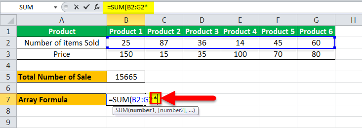
- In cell B7, type =SUM and press the “tab” button on the keyboard. It may open up the sum formula.

- Select the cell range from B2 to G2.

- Now, put an asterisk “*” sign after B2:G2 to multiply.

- Select the cell range from B3 to G3.

- Instead of pressing the “Enter” key, press “CTRL + SHIFT + ENTER.”

As a result, Excel may provide the total sales value by multiplying the number of products by the price in each column and summing them up. For example, in the highlighted section, we can see that Excel has created an array for cell range B2 to G2 and B3 to G3.

The above example explains how Excel array formulas return a single value for an array or set of data.


Example #2
With the same data, what if the owner wants to know the sales for each product separately, like sales of products 1 and 2?

He can either go a long way. In each cell, perform a function that will calculate the sales value.
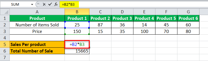
The equation mentioned in cell B5 will be required to repeat for cells C4, D4, etc.
Again, it would be a tedious task if it were larger data.
In this example, we will learn how array formulas in Excel return multiple values for a set of arrays.

#1 – Select the cells where we want our subtotals, i.e., per product sales for each product. In this case, it is a cell range B8 to G8.

#2 – Type an equal to sign “=” a
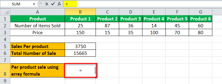
#3 –Select cell range B2 to G2.

#4 – Type an asterisk “*” sign after B2:G2.

#5 – Now, select cell range B3 to G3.

#6 – Do not press the “Enter” key for the array formula. Press “CTRL + SHIFT + ENTER” for array formula.

The above example explains how an array formula can return multiple values for an array in Excel.
Cells B6 to G6 are an array.
Example #3
For the same restaurant owner, he has the restaurant sales data for six months Jan, Feb, March, April, May, and June. He wants to know the average growth rate for sales.
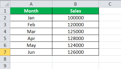
The owner can normally subtract the sales value of Feb month to Jan in cell C2 and then calculate the average.

Again, it would be a tiresome task if this were larger data. So let us do this with the array in Excel formulas.
#1 – In cell D8, type =average. Then, press the “tab” button.

#2 – To calculate growth, we will need to subtract the values of one month from the previous month to select the cell range from B3 to B7.

#3 – Put a subtract (-) sign after B3:B7,

#4 – Now, select cells from B2 to B6.
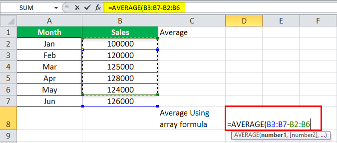
#5 – As for the array in Excel, do not press the “Enter” key. Press “CTRL + SHIFT + ENTER.”

Array formulas in Excel easily calculated the average growth for the sales without any hassle.
The owner now does not require calculating each month’s growth and performs the average function after that.
Things to Remember
- These are also known as CSE Formulas or Control Shift Enter ExcelCtrl-Shift Enter In Excel is a shortcut command that facilitates implementing the array formula in the excel function to execute an intricate computation of the given data. Altogether it transforms a particular data into an array format in excel with multiple data values for this purpose.read more Formulas.
- Do not make parenthesis for an array; Excel itself does that. It would return an error or incorrect value.
- Entering the parenthesis “{“manually, Excel will treat it as a text.
- Do not press the “Enter” key. Instead, press “CTRL + SHIFT + Enter” to use an array formula.
- We cannot change the cell of an array. So, to modify an array formula, either modify the formula from the function bar or delete the formula and redesign it in the desired format.
Recommended Articles
This article is a step-by-step guide to Array formulas in Excel. Here, we discuss how to use array in Excel using basic SUM and AVERAGE formulas and use it to solve array in Excel along with Excel examples and downloadable Excel templates. You may also look at these useful functions in Excel: –
- What is Name Range in Excel?
- Redim Array in Excel VBA
- Excel Formula Cheat Sheet
- VBA Array Function
An array in Excel is a structure that holds a collection of values. Arrays can be mapped perfectly to ranges in a spreadsheet, which is why they are so important in Excel. An array can be thought of as a row of values, a column of values, or a combination of rows and columns with values. All cell references like A1:A5 and C1:F5 have underlying arrays, though the array structure is invisible in most contexts.
Example
In the example above, the three ranges map to arrays in a «row by column» scheme like this:
B5:D5 // 1 row x 3 columns
B8:B10 // 3 rows x 1 column
B13:D14  // 2 rows x 3 columns
If we display the values in these ranges as arrays, we have:
B5:D5={"red","green","blue"}
B8:B10={"red";"green";"blue"}
B13:D14={10,20,30;40,50,60}
Notice arrays must represent a rectangular structure.
Array syntax
All arrays in Excel are wrapped in curly brackets {} and the delimiters between array elements indicate rows and/or columns. In the US version of Excel, a comma (,) separates columns and a semicolon (;) separates rows. For example, both arrays below contain numbers 1-3, but one is horizontal and one is vertical:
{1,2,3} // columns (horizontal)
{1;2;3} // rows (vertical)
Text values in an array appear in double quotes («») like this:
{"a","b","c"}
To «see» the array associated with a range, start a formula with an equal sign (=) and select the range. Then use the F9 key to inspect the underlying array. You can also use the ARRAYTOTEXT function to show how columns and rows are represented. Set format to 1 (strict) to see the complete array.
Delimiters in other languages
In other language versions of Excel, the delimiters for rows and column can vary. For example, the Spanish version of Excel uses a backslash () for columns and a semicolon (;) for rows:
{123} // columns
{1;2;3} // rows
Arrays in formulas
Since arrays map directly to ranges, all formulas work with arrays in some way, though it isn’t always obvious. A simple example is a formula that uses the SUM function to sum the range A1:A5, which contains 10,15,20,25,30. Inside SUM, the range resolves to an array of values. SUM then sums all values in the array and returns a single result of 100:
=SUM(A1:A5)
=SUM({10;15;20;25;30})
=100
Note: you can use the F9 key to «see» arrays in your Excel formulas. See this video for a demo on using F9 to debug.
Array formulas
Array formulas involve an operation that delivers an array of results. For example, here is a simple array formula that returns the total count of characters in the range A1:A5:
=SUM(LEN(A1:A5))
Inside the LEN function, A1:A5 is expanded to an array of values. The LEN function then generates a character count for each value and returns an array of 5 results. The SUM function then returns the sum of all items in the array.
Dynamic arrays
With the introduction of Dynamic Array formulas in Excel, arrays have become more important, since it is easier than ever to write formulas that work with multiple results at the same time.