Set all row heights in excel

If you find yourself needing to expand or reduce Excel’s row widths and column heights, there are several ways to adjust them. The table below shows the minimum, maximum and default sizes for each based on a point scale.

Type	Min	Max	Default
Column	0 (hidden)	255	8.43
Row	0 (hidden)	409	15.00

Notes:

If you are working in Page Layout view (View tab, Workbook Views group, Page Layout button), you can specify a column width or row height in inches, centimeters and millimeters. The measurement unit is in inches by default. Go to File > Options > Advanced > Display > select an option from the Ruler Units list. If you switch to Normal view, then column widths and row heights will be displayed in points.
Individual rows and columns can only have one setting. For example, a single column can have a 25 point width, but it can’t be 25 points wide for one row, and 10 points for another.

Set a column to a specific width

Select the column or columns that you want to change.
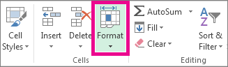
On the Home tab, in the Cells group, click Format.
Under Cell Size, click Column Width.
In the Column width box, type the value that you want.
Click OK.

Tip: To quickly set the width of a single column, right-click the selected column, click Column Width, type the value that you want, and then click OK.

Select the column or columns that you want to change.
On the Home tab, in the Cells group, click Format.
Under Cell Size, click AutoFit Column Width.

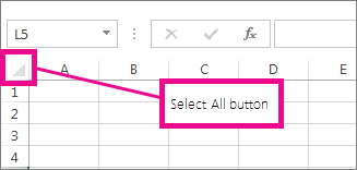
Note: To quickly autofit all columns on the worksheet, click the Select All button, and then double-click any boundary between two column headings.

Select a cell in the column that has the width that you want to use.
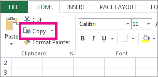
Press Ctrl+C, or on the Home tab, in the Clipboard group, click Copy.
Right-click a cell in the target column, point to Paste Special, and then click the Keep Source Columns Widths button.

The value for the default column width indicates the average number of characters of the standard font that fit in a cell. You can specify a different number for the default column width for a worksheet or workbook.

Do one of the following:
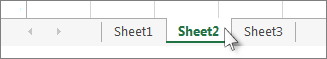
- To change the default column width for a worksheet, click its sheet tab.
- To change the default column width for the entire workbook, right-click a sheet tab, and then click Select All Sheets on the shortcut menu.
On the Home tab, in the Cells group, click Format.
Under Cell Size, click Default Width.
In the Standard column width box, type a new measurement, and then click OK.

Do one of the following:

To change the width of one column, drag the boundary on the right side of the column heading until the column is the width that you want.
To change the width of multiple columns, select the columns that you want to change, and then drag a boundary to the right of a selected column heading.
To change the width of columns to fit the contents, select the column or columns that you want to change, and then double-click the boundary to the right of a selected column heading.
To change the width of all columns on the worksheet, click the Select All button, and then drag the boundary of any column heading.

Select the row or rows that you want to change.
On the Home tab, in the Cells group, click Format.
Under Cell Size, click Row Height.
In the Row height box, type the value that you want, and then click OK.

Select the row or rows that you want to change.
On the Home tab, in the Cells group, click Format.
Under Cell Size, click AutoFit Row Height.

Tip: To quickly autofit all rows on the worksheet, click the Select All button, and then double-click the boundary below one of the row headings.

Do one of the following:

To change the row height of one row, drag the boundary below the row heading until the row is the height that you want.
To change the row height of multiple rows, select the rows that you want to change, and then drag the boundary below one of the selected row headings.
To change the row height for all rows on the worksheet, click the Select All button, and then drag the boundary below any row heading.
To change the row height to fit the contents, double-click the boundary below the row heading.

Top of Page

If you prefer to work with column widths and row heights in inches, you should work in Page Layout view (View tab, Workbook Views group, Page Layout button). In Page Layout view, you can specify a column width or row height in inches. In this view, inches are the measurement unit by default, but you can change the measurement unit to centimeters or millimeters.

In Excel 2007, click the Microsoft Office Button > Excel Options> Advanced.
In Excel 2010, go to File > Options > Advanced.

Set a column to a specific width

Select the column or columns that you want to change.
On the Home tab, in the Cells group, click Format.
Under Cell Size, click Column Width.
In the Column width box, type the value that you want.

Select the column or columns that you want to change.
On the Home tab, in the Cells group, click Format.
Under Cell Size, click AutoFit Column Width.

Tip To quickly autofit all columns on the worksheet, click the Select All button and then double-click any boundary between two column headings.

Select a cell in the column that has the width that you want to use.
On the Home tab, in the Clipboard group, click Copy, and then select the target column.
On the Home tab, in the Clipboard group, click the arrow below Paste, and then click Paste Special.
Under Paste, select Column widths.

Do one of the following:
- To change the default column width for a worksheet, click its sheet tab.
- To change the default column width for the entire workbook, right-click a sheet tab, and then click Select All Sheets on the shortcut menu.
On the Home tab, in the Cells group, click Format.
Under Cell Size, click Default Width.
In the Default column width box, type a new measurement.

Tip If you want to define the default column width for all new workbooks and worksheets, you can create a workbook template or a worksheet template, and then base new workbooks or worksheets on those templates. For more information, see Save a workbook or worksheet as a template.

Do one of the following:

To change the width of one column, drag the boundary on the right side of the column heading until the column is the width that you want.
To change the width of multiple columns, select the columns that you want to change, and then drag a boundary to the right of a selected column heading.
To change the width of columns to fit the contents, select the column or columns that you want to change, and then double-click the boundary to the right of a selected column heading.
To change the width of all columns on the worksheet, click the Select All button, and then drag the boundary of any column heading.

Select the row or rows that you want to change.
On the Home tab, in the Cells group, click Format.
Under Cell Size, click Row Height.
In the Row height box, type the value that you want.

Select the row or rows that you want to change.
On the Home tab, in the Cells group, click Format.
Under Cell Size, click AutoFit Row Height.

Tip To quickly autofit all rows on the worksheet, click the Select All button and then double-click the boundary below one of the row headings.

Do one of the following:

To change the row height of one row, drag the boundary below the row heading until the row is the height that you want.
To change the row height of multiple rows, select the rows that you want to change, and then drag the boundary below one of the selected row headings.
To change the row height for all rows on the worksheet, click the Select All button, and then drag the boundary below any row heading.
To change the row height to fit the contents, double-click the boundary below the row heading.

Top of Page

Change the column width or row height in Excel

You can manually adjust the column width or row height or automatically resize columns and rows to fit the data.

Note: The boundary is the line between cells, columns, and rows. If a column is too narrow to display the data, you will see ### in the cell.

Resize rows

Select a row or a range of rows.
On the Home tab, select Format > Row Width (or Row Height).
Type the row width and select OK.

Resize columns

Select a column or a range of columns.
On the Home tab, select Format > Column Width (or Column Height).
Type the column width and select OK.

Automatically resize all columns and rows to fit the data

Select the Select All button at the top of the worksheet, to select all columns and rows.
Double-click a boundary. All columns or rows resize to fit the data.

Need more help?

You can always ask an expert in the Excel Tech Community or get support in the Answers community.

Начнём с теории

Если обратиться к документации по VBA для Microsoft Office, то можно увидеть, что высоту ряда так или иначе можно получить через два свойства:

RowHeight — Returns or sets the height of the first row in the range specified, measured in points. Read/write Double;
Height — Returns a Double value that represents the height, in points, of the range. Read-only.

Причём если заглянуть ещё и сюда: Excel specifications and limits. То можно обнаружить, что максимальная высота ряда составляет 409 точек. Это к сожалению далеко не единственный случай, когда официальные документы Microsoft немножко лукавят. На самом деле в коде Excel максимальная высота ряда задана как 2047 пикселя, что в точках будет 1535.25. А максимальный размер шрифта 409.55 пунктов. Получить ряд такой огромной высоты простым присваиванием в VBA/Interop не получится, но можно взять ряд, задать его первой ячейке шрифт Cambria Math, а размер шрифта выставить в 409.55 пунктов. Тогда Excel своим хитрым алгоритмом посчитает высоту ряда на основе формата ячейки, получит число превышающее 2047 пикселей (поверьте на слово) и сам выставит у ряда максимально возможную высоту. Если спросить высоту этого ряда через UI, то Excel соврёт что высота 409.5 точек, но если запросить высоту ряда через VBA, то получится честные 1535,25 точек, что равняется 2047 пикселям. Правда после сохранения документа высота всё равно сбросится до 409,5 точек. Эту манипуляцию можно пронаблюдать вот на этом видео: http://recordit.co/ivnFEsELLI

Я не зря упомянул в предыдущем абзаце пиксели. Excel на самом деле хранит и рассчитывает размеры ячеек в целых числах (он вообще максимально всё делает в целых числах). Чаще всего это пиксели, умноженные на некоторый коэффициент. Интересно, что Excel хранит масштаб внешнего вида в виде обыкновенной дроби, например, масштаб 75% будет храниться как два числа 3 и 4. И когда надо будет вывести на экран ряд, Excel возьмёт высоту ряда как целое число пикселей, умножит на 3 и разделит на 4. Но выполнять эту операцию он будет уже в самом конце от этого создаётся эффект, что всё считается в дробных числах. Чтобы в этом убедиться напишите в VBA вот такой код:

w.Rows(1).RowHeight = 75.375
Debug.Print w.Rows(1).Height

VBA выдаст 75, т.к. 75,375 точек будет 100,5 пикселей, а Excel такое себе позволить не может и отбросит дробную часть до 100 пикселей. Когда VBA будет запрашивать высоту ряда в точках, Excel честно переведёт 100 пикселей в точки и вернёт 75.

В принципе мы уже подобрались к тому, чтобы написать класс на C#, который будет описывать информацию о высоте ряда:

class RowHeightInfo {
    public ushort Value { get; set; } //высота ряда в целых пикселях, умноженная на 4.
    public ushort Flags { get; set; } //дополнительные флаги
}

Вам пока что придётся поверить мне на слово, но в Excel высота ряда хранится именно так. Т.е., если задано, что высота ряда 75 точек, в пикселях это будет 100, то в Value будет хранится 400. Что обозначают все биты в Flags я до конца не выяснил (выяснять значения флагов сложно и долго), но знаю точно, что 0x4000 выставляется для рядов у которых высота задана вручную, а 0x2000 — выставляется у скрытых рядов. В целом у видимых рядов с заданной вручную высотой Flags чаще всего равняется 0x4005, а для рядов у которых высота высчитывается на основе форматирования Flags равняется либо 0xA, либо 0x800E.

Спрашиваем высоту ряда

Теперь в принципе можно взглянуть на метод из excel.exe, который возвращает высоту ряда по его индексу (спасибо HexRays за красивый код):

int __userpurge GetRowHeight@<eax>(signed int rowIndex@<edx>, SheetLayoutInfo *sheetLayoutInfo@<esi>, bool flag)
{
  RowHeightInfo *rowHeightInfo; // eax
  int result; // ecx

  if ( sheetLayoutInfo->dword1A0 )
    return sheetLayoutInfo->defaultFullRowHeightMul4 | (~(sheetLayoutInfo->defaultRowDelta2 >> 14 << 15) & 0x8000);
  if ( rowIndex < sheetLayoutInfo->MinRowIndexNonDefault )
    return sheetLayoutInfo->defaultFullRowHeightMul4 | (~(sheetLayoutInfo->defaultRowDelta2 >> 14 << 15) & 0x8000);
  if ( rowIndex >= sheetLayoutInfo->MaxRowIndexNonDefault )
    return sheetLayoutInfo->defaultFullRowHeightMul4 | (~(sheetLayoutInfo->defaultRowDelta2 >> 14 << 15) & 0x8000);
  rowHeightInfo = GetRowHeightCore(sheetLayoutInfo, rowIndex);
  if ( !rowHeightInfo )
    return sheetLayoutInfo->defaultFullRowHeightMul4 | (~(sheetLayoutInfo->defaultRowDelta2 >> 14 << 15) & 0x8000);
  result = 0;
  if ( flag || !(rowHeightInfo->Flags & 0x2000) )
    result = rowHeightInfo->Value;
  if ( !(rowHeightInfo->Flags & 0x4000) )
    result |= 0x8000u;
  return result;
}

Что такое dword1A0 я так и не выяснил, т.к. не смог найти место где этот флаг выставляется
Что такое defaultRowDelta2 для меня тоже до сих пор остаётся загадкой. Когда excel рассчитывает высоту ряда на основе формата, то представляет её как сумму двух чисел. defaultRowDelta2 — это второе число из этой суммы для стандартной высоты ряда. Значение параметра flag тоже загадочно, т.к. везде где я видел вызов этого метода в flag передавался false.
В этом методе также появляется класс SheetLayoutInfo. Я его назвал именно так, потому что в нём хранится много всякой информации о внешнем виде листа. В SheetLayoutInfo есть такие поля как:

DefaultFullRowHeightMul4 — стандартная высота ряда;
MinRowIndexNonDefault — индекс первого ряда, у которого высота отличается от стандартной;
MaxRowIndexNonDefault — индекс ряда, следующего за последним, у которого высота отличается от стандартной;
DefaultRowDelta2 — та самая часть от суммы стандартной высоты ряда.
GroupIndexDelta — об этом позже

В принципе логика данного метода вполне понятна:

Если индекс ряда меньше первого с нестандартной высотой, то возвращаем стандартную;
Если индекс ряда больше последнего с нестандартной высотой, то возвращаем стандартную;
В противном случае получаем объект rowHeightInfo для ряда из метода GetRowHeightCore;
Если rowHeightInfo == null возвращаем стандартную высоту ряда;
Тут магия с флагами, но в общем виде мы возвращаем то, что находится в rowHeightInfo.Value и выставляем 16-й бит в ответе, если высота ряда не была задана вручную.

Если переписать этот код на C#, то получится примерно следующее:

const ulong HiddenRowMask = 0x2000;
const ulong CustomHeightMask = 0x4000;
const ushort DefaultHeightMask = 0x8000;
public static ushort GetRowHeight(int rowIndex, SheetLayoutInfo sheetLayoutInfo) {
    ushort defaultHeight = (ushort) (sheetLayoutInfo.DefaultFullRowHeightMul4 | (~(sheetLayoutInfo.DefaultRowDelta2 >> 14 << 15) & DefaultHeightMask));
    if (rowIndex < sheetLayoutInfo.MinRowIndexNonDefault)
        return defaultHeight;
    if (rowIndex >= sheetLayoutInfo.MaxRowIndexNonDefault)
        return defaultHeight;
    RowHeightInfo rowHeightInfo = GetRowHeightCore(sheetLayoutInfo, rowIndex);
    if (rowHeightInfo == null)
        return defaultHeight;
    ushort result = 0;
    if ((rowHeightInfo.Flags & HiddenRowMask) == 0)
        result = rowHeightInfo.Value;
    if ((rowHeightInfo.Flags & CustomHeightMask) == 0)
        result |= DefaultHeightMask;
    return result;
}

Теперь можно взглянуть что происходит внутри GetRowHeightCore:

RowHeightInfo *__fastcall GetRowHeightCore(SheetLayoutInfo *sheetLayoutInfo, signed int rowIndex)
{
  RowHeightInfo *result; // eax
  RowsGroupInfo *rowsGroupInfo; // ecx
  int rowInfoIndex; // edx

  result = 0;
  if ( rowIndex < sheetLayoutInfo->MinRowIndexNonDefault || rowIndex >= sheetLayoutInfo->MaxRowIndexNonDefault )
    return result;
  rowsGroupInfo = sheetLayoutInfo->RowsGroups[sheetLayoutInfo-GroupIndexDelta + (rowIndex >> 4)];
  result = 0;
  if ( !rowsGroupInfo )
    return result;
  rowInfoIndex = rowsGroupInfo->Indices[rowIndex & 0xF];
  if ( rowInfoIndex )
    result = (rowsGroupInfo + 8 * (rowInfoIndex + rowsGroupInfo->wordBA + rowsGroupInfo->wordBC - rowsGroupInfo->wordB8));
  return result;
}

Опять в начале Excel проверяет находится ли индекс ряда среди рядов с изменённой высотой и если нет, то возвращает null.
Находит нужную группу рядов, если такой группы нет, то возвращает null.
Получает индекс ряда в группе.
Далее по индексу ряда находит нужный объект класса RowHeightInfo. wordBA, wordBC, wordB8 — какие-то константы. Они изменяются только вместе с историей. В принципе на понимание алгоритма они не влияют.

Тут стоит отклониться от темы и рассказать подробнее про RowsGroupInfo. Excel хранит RowHeightInfo группами по 16 штук, где i-я группа, представленная классом RowsGroupInfo, будет хранить в себе информацию о рядах с i × 16 до i × 16 + 15 включительно.

Но информация о высоте рядов в RowsGroupInfo хранится несколько необычным способом. Скорее всего из-за необходимости поддерживать историю в Excel.

В RowsGroupInfo есть три важных поля: Indices, HeightInfos, и RowsCount, второе в коде выше не видно (оно должно быть в этой строчке: (rowsGroupInfo + 8 × (…)), т.к. rowInfoIndex может принимать очень разные значения, я видел даже больше 1000 и я понятия не имею как в IDA задать такую структуру. Поле RowsCount вообще в коде выше не встречается, но именно там хранится сколько реально нестандартных рядов хранится в группе.
Кроме того, в SheetLayoutInfo есть GroupIndexDelta — разница между реальным индексом группы и индексом первой группы с изменённой высотой ряда.

В поле Indices хранятся смещения RowHeightInfo для каждого индекса ряда внутри группы. Они хранятся там по порядку, а вот в HeightInfos RowHeightInfo уже хранятся в порядке изменения.

Допустим у нас есть новый пустой лист и мы каким-то образом изменили высоту ряда номер 23. Это ряд лежит во второй группе из 16 рядов, тогда:

Excel определит индекс группы для этого ряда. В текущем случае индекс будет равен 1 и изменит GroupIndexDelta = -1.
Создаст для группы рядов объект класса RowsGroupInfo и положит его в sheetLayoutInfo->RowsGroups под индексом 0 (sheetLayoutInfo->GroupIndexDelta + 1);
В RowsGroupInfo Excel выделит память под 16 4-х байтовых Indices, под RowsCount, wordBA, wordBC и wordB8 и т.д..;
Потом Excel вычисляет индекс ряда в группе через операцию побитового И (это сильно быстрее чем брать остаток от деления): rowIndex & 0xF. Искомый индекс в группе будет равняться: 23 & 0xF = 7;
После этого Excel получает смещение для индекса 7: offset = Indices[7]. Если offset = 0, то Excel выделяет 8 байт в конце RowsGroupInto, увеличивает RowsCount на единицу и записывает новое смещение в Indices[7]. В любом случае в конце Excel запишет по смещению в RowsGroupInfo информацию о новой высоте ряда и флагах.

Сам класс RowsGroupInfo на C# выглядел бы вот так:

class RowsGroupInfo {
    public int[] Indices { get; }
    public List<RowHeightInfo> HeightInfos { get; }

    public RowsGroupInfo() {
        Indices = new int[SheetLayoutInfo.MaxRowsCountInGroup];
        HeightInfos = new List<RowHeightInfo>();
        for (int i = 0; i < SheetLayoutInfo.MaxRowsCountInGroup; i++) {
            Indices[i] = -1;
        }
    }
}

Метод GetRowHeightCore выглядел бы вот так:

static RowHeightInfo GetRowHeightCore(SheetLayoutInfo sheetLayoutInfo, int rowIndex) {
    if (rowIndex < sheetLayoutInfo.MinRowIndexNonDefault || rowIndex >= sheetLayoutInfo.MaxRowIndexNonDefault)
        return null;
    RowsGroupInfo rowsGroupInfo = sheetLayoutInfo.RowsGroups[sheetLayoutInfo.GroupIndexDelta + (rowIndex >> 4)];
    if (rowsGroupInfo == null)
        return null;
    int rowInfoIndex = rowsGroupInfo.Indices[rowIndex & 0xF];
    return rowInfoIndex != -1 ? rowsGroupInfo.HeightInfos[rowInfoIndex] : null;
}

И вот так выглядел бы SetRowHeight (его код из excel.exe я не приводил):

public static void SetRowHeight(int rowIndex, ushort newRowHeight, ushort flags, SheetLayoutInfo sheetLayoutInfo) {
    sheetLayoutInfo.MaxRowIndexNonDefault = Math.Max(sheetLayoutInfo.MaxRowIndexNonDefault, rowIndex + 1);
    sheetLayoutInfo.MinRowIndexNonDefault = Math.Min(sheetLayoutInfo.MinRowIndexNonDefault, rowIndex);
    int realGroupIndex = rowIndex >> 4;
    if (sheetLayoutInfo.RowsGroups.Count == 0) {
        sheetLayoutInfo.RowsGroups.Add(null);
        sheetLayoutInfo.GroupIndexDelta = -realGroupIndex;
    }
    else if (sheetLayoutInfo.GroupIndexDelta + realGroupIndex < 0) {
        int bucketSize = -(sheetLayoutInfo.GroupIndexDelta + realGroupIndex);
        sheetLayoutInfo.RowsGroups.InsertRange(0, new RowsGroupInfo[bucketSize]);
        sheetLayoutInfo.GroupIndexDelta = -realGroupIndex;
    }
    else if (sheetLayoutInfo.GroupIndexDelta + realGroupIndex >= sheetLayoutInfo.RowsGroups.Count) {
        int bucketSize = sheetLayoutInfo.GroupIndexDelta + realGroupIndex - sheetLayoutInfo.RowsGroups.Count + 1;
        sheetLayoutInfo.RowsGroups.AddRange(new RowsGroupInfo[bucketSize]);
    }
    RowsGroupInfo rowsGroupInfo = sheetLayoutInfo.RowsGroups[sheetLayoutInfo.GroupIndexDelta + realGroupIndex];
    if (rowsGroupInfo == null) {
        rowsGroupInfo = new RowsGroupInfo();
        sheetLayoutInfo.RowsGroups[sheetLayoutInfo.GroupIndexDelta + realGroupIndex] = rowsGroupInfo;
    }
    int rowInfoIndex = rowsGroupInfo.Indices[rowIndex & 0xF];
    RowHeightInfo rowHeightInfo;
    if (rowInfoIndex == -1) {
        rowHeightInfo = new RowHeightInfo();
        rowsGroupInfo.HeightInfos.Add(rowHeightInfo);
        rowsGroupInfo.Indices[rowIndex & 0xF] = rowsGroupInfo.HeightInfos.Count - 1;
    }
    else {
        rowHeightInfo = rowsGroupInfo.HeightInfos[rowInfoIndex];
    }
    rowHeightInfo.Value = newRowHeight;
    rowHeightInfo.Flags = flags;
}

Немного практики

После разобранного выше примера с изменением высоты ряда 23 в памяти Excel будет примерно такая картина (я задал ряду 23 высоту 75 точек):

sheetLayoutInfo

DefaultFullRowHeightMul4 = 80
DefaultRowDelta2 = 5
MaxRowIndexNonDefault = 24
MinRowIndexNonDefault = 23
GroupIndexDelta = -1
RowsGroups Count = 1
- [0] RowsGroupInfo
- HeightInfos Count = 1
  - [0] RowHeightInfo
  - Flags = 0x4005
  - Value = 100
- Indices
  - [0] = -1
  - [1] = -1
  - [2] = -1
  - [3] = -1
  - [4] = -1
  - [5] = -1
  - [6] = -1
  - [7] = 0
  - [8] = -1
  - [9] = -1
  - [10] = -1
  - [11] = -1
  - [12] = -1
  - [13] = -1
  - [14] = -1
  - [15] = -1

Здесь и в следующем примере я буду выкладывать схематичное представление о том, как выглядят данные в памяти Excel, сделанное в Visual Studio из самописных классов, потому что прямой дамп из памяти не сильно информативен.
Теперь попробуем спрятать ряд 23. Для этого надо выставить бит 0x2000 у Flags. Будем изменять память на живую. Результат можно увидеть на этом видео: http://recordit.co/79vYIbwbzB.
При любом скрытии рядов Excel поступает также.
Теперь зададим высоту ряда не явно, а через формат ячейки. Пускай у ячейки A20 шрифт станет высотой 40 пунктов, тогда высота ячейки в точках станет 45,75 и в памяти Excel будет примерно такое:

sheetLayoutInfo

DefaultFullRowHeightMul4 = 80
DefaultRowDelta2 = 5
MaxRowIndexNonDefault = 24
MinRowIndexNonDefault = 20
GroupIndexDelta = -1
RowsGroups Count = 1
- [0] RowsGroupInfo
- HeightInfos Count = 2
  - [0] RowHeightInfo
  - Flags = 0x4005
  - Value = 100
  - [1] RowHeightInfo
  - Flags = 0x800E
  - Value = 244
- Indices
  - [0] = -1
  - [1] = -1
  - [2] = -1
  - [3] = -1
  - [4] = 1
  - [5] = -1
  - [6] = -1
  - [7] = 0
  - [8] = -1
  - [9] = -1
  - [10] = -1
  - [11] = -1
  - [12] = -1
  - [13] = -1
  - [14] = -1
  - [15] = -1

Можно заметить, что Excel всегда хранит высоту ряда, если она не стандартная. Даже если высота не задана явно, а рассчитывается на основе содержимого ячеек или формата, то Excel всё равно посчитает её один раз и занесёт результат в соответствующую группу.

Разбираемся со вставкой/удалением рядов

Интересно было бы разобрать что происходит при вставке/удалении рядов. Соответствующий код в excel.exe найти несложно, но разбирать его не было желания, можете сами взглянуть на часть из него:

sub_305EC930

Флаг a5 определяет какая именно сейчас происходит операция.

int __userpurge sub_305EC930@<eax>(int a1@<eax>, int a2@<edx>, int a3@<ecx>, int a4, int a5, int a6)
{
  int v6; // esi
  int v7; // ebx
  int v8; // edi
  int v9; // edx
  int v10; // ecx
  size_t v11; // eax
  _WORD *v12; // ebp
  size_t v13; // eax
  size_t v14; // eax
  int v15; // eax
  unsigned __int16 *v16; // ecx
  _WORD *v17; // eax
  _WORD *v18; // ecx
  int v19; // edx
  __int16 v20; // bx
  int v21; // eax
  _WORD *v22; // ecx
  int v24; // edx
  int v25; // eax
  int v26; // esi
  int v27; // ebx
  size_t v28; // eax
  int v29; // ebp
  size_t v30; // eax
  int v31; // esi
  size_t v32; // eax
  int v33; // eax
  unsigned __int16 *v34; // ecx
  int v35; // eax
  _WORD *v36; // edx
  _WORD *v37; // ecx
  int v38; // eax
  __int16 v39; // bx
  int v40; // eax
  _WORD *v41; // ecx
  int v42; // [esp+10h] [ebp-48h]
  int v43; // [esp+10h] [ebp-48h]
  int v44; // [esp+14h] [ebp-44h]
  char v45; // [esp+14h] [ebp-44h]
  int Dst[16]; // [esp+18h] [ebp-40h]
  int v47; // [esp+5Ch] [ebp+4h]
  int v48; // [esp+60h] [ebp+8h]

  v6 = a1;
  v7 = a1 & 0xF;
  v8 = a2;
  if ( !a5 )
  {
    v24 = a4 - a1;
    v25 = a1 - a3;
    v43 = a4 - v6;
    if ( v7 >= v25 )
      v7 = v25;
    v47 = a4 - v7;
    v26 = v6 - v7;
    v27 = v7 + 1;
    v48 = v27;
    if ( !v8 )
      return v27;
    v28 = 4 * v24;
    if ( (4 * v24) > 0x40 )
      v28 = 64;
    v45 = v27 + v26;
    v29 = (v27 + v26) & 0xF;
    memmove(Dst, (v8 + 4 * v29), v28);
    v30 = 4 * v27;
    if ( (4 * v27) > 0x40 )
      v30 = 64;
    v31 = v26 & 0xF;
    memmove((v8 + 4 * (v47 & 0xF)), (v8 + 4 * v31), v30);
    v32 = 4 * v43;
    if ( (4 * v43) > 0x40 )
      v32 = 64;
    memmove((v8 + 4 * v31), Dst, v32);
    if ( !a6 )
      return v48;
    v33 = v29;
    if ( v29 < v29 + v43 )
    {
      v34 = (v8 + 4 * v29 + 214);
      do
      {
        Dst[v33++] = *v34 >> 15;
        v34 += 2;
      }
      while ( v33 < v29 + v43 );
    }
    v35 = (v45 - 1) & 0xF;
    if ( v35 >= v31 )
    {
      v36 = (v8 + 4 * ((v27 + v47 - 1) & 0xF) + 214);
      v37 = (v8 + 4 * ((v45 - 1) & 0xF) + 214);
      v38 = v35 - v31 + 1;
      do
      {
        v39 = *v37 ^ (*v37 ^ *v36) & 0x7FFF;
        v37 -= 2;
        *v36 = v39;
        v36 -= 2;
        --v38;
      }
      while ( v38 );
      v27 = v48;
    }
    v40 = v31;
    if ( v31 >= v31 + v43 )
      return v27;
    v41 = (v8 + 4 * v31 + 214);
    do
    {
      *v41 = *v41 & 0x7FFF | (LOWORD(Dst[v40++]) << 15);
      v41 += 2;
    }
    while ( v40 < v31 + v43 );
    return v27;
  }
  v9 = a1 - a4;
  v10 = a3 - a1;
  v42 = a1 - a4;
  v48 = 16 - v7;
  if ( 16 - v7 >= v10 )
    v48 = v10;
  if ( !v8 )
    return v48;
  v11 = 4 * v9;
  if ( (4 * v9) > 0x40 )
    v11 = 64;
  v12 = (v8 + 4 * (a4 & 0xF));
  v44 = a4 & 0xF;
  memmove(Dst, v12, v11);
  v13 = 4 * v48;
  if ( (4 * v48) > 0x40 )
    v13 = 64;
  memmove(v12, (v8 + 4 * v7), v13);
  v14 = 4 * v42;
  if ( (4 * v42) > 0x40 )
    v14 = 64;
  memmove((v8 + 4 * ((a4 + v48) & 0xF)), Dst, v14);
  if ( !a6 )
    return v48;
  v15 = a4 & 0xF;
  if ( v44 < v44 + v42 )
  {
    v16 = (v8 + 4 * v44 + 214);
    do
    {
      Dst[v15++] = *v16 >> 15;
      v16 += 2;
    }
    while ( v15 < v44 + v42 );
  }
  if ( v7 < v48 + v7 )
  {
    v17 = (v8 + 4 * v7 + 214);
    v18 = v12 + 107;
    v19 = v48;
    do
    {
      v20 = *v17 ^ (*v17 ^ *v18) & 0x7FFF;
      v17 += 2;
      *v18 = v20;
      v18 += 2;
      --v19;
    }
    while ( v19 );
  }
  v21 = a4 & 0xF;
  if ( v44 >= v44 + v42 )
    return v48;
  v22 = (v8 + 4 * (v44 + v48) + 214);
  do
  {
    *v22 = *v22 & 0x7FFF | (LOWORD(Dst[v21++]) << 15);
    v22 += 2;
  }
  while ( v21 < v44 + v42 );
  return v48;
}

К тому же по внешнему виду можно примерно понять что там происходит, а остальное добить по косвенным признакам.
Попытаемся обозначить эти косвенные признаки. Сначала зададим высоту для рядов с 16 по 64 включительно в случайном порядке. Потом перед рядом под индексом 39 вставим новый ряд. Новый ряд будет копировать высоту у ряда 38.
Посмотрим на информацию в группах рядов до и после добавления ряда, я выделил жирным различия:

До добавления ряда	После добавления ряда
Смещения в первой группе:	Смещения в первой группе:
0E, 04, 07, 00, 05, 0A, 09, 0F, 03, 06, 08, 0D, 01, 0B, 0C, 02	0E, 04, 07, 00, 05, 0A, 09, 0F, 03, 06, 08, 0D, 01, 0B, 0C, 02
Значения высот рядов в первой группе:	Значения высот рядов в первой группе:
05, 2B, 35, 45, 4B, 50, 5B, 6B, 7B, 8B, A5, AB, B0, B5, E0, 100	05, 2B, 35, 45, 4B, 50, 5B, 6B, 7B, 8B, A5, AB, B0, B5, E0, 100
Смещения во второй группе:	Смещения во второй группе:
06, 02, 0E, 09, 01, 07, 0F, 0C, 00, 0A, 04, 0B, 03, 08, 0D, 05	06, 02, 0E, 09, 01, 07, 0F, 05, 0C, 00, 0A, 04, 0B, 03, 08, 0D
Значения высот рядов во второй группе:	Значения высот рядов во второй группе:
10, 15, 20, 25, 30, 75, 85, 90, 9B, A0, C5, CB, D0, D5, E5, F0	10, 15, 20, 25, 30, F0, 85, 90, 9B, A0, C5, CB, D0, D5, E5, F0
Смещения в третьей группе:	Смещения в третьей группе:
0C, 08, 0E, 07, 0A, 01, 06, 0F, 09, 0D, 00, 05, 0B, 02, 04, 03	03, 0C, 08, 0E, 07, 0A, 01, 06, 0F, 09, 0D, 00, 05, 0B, 02, 04
Значения высот рядов в третьей группе:	Значения высот рядов в третьей группе:
0B, 1B, 3B, 40, 55, 60, 65, 70, 80, 95, BB, C0, DB, EB, F5, FB	0B, 1B, 3B, 75, 55, 60, 65, 70, 80, 95, BB, C0, DB, EB, F5, FB
Смещения в четвёртой группе:	Смещения в четвёртой группе:
_	00
Значения высот рядов в четвёртой группе:	Значения высот рядов в четвёртой группе:
_	40

Получается то, что и ожидалось: Excel вставляет во вторую группу новый ряд с индексом 7 (39 & 0xF), у которого смещение равняется 0x05, копирует высоту ряда у индекса 6, при этом последний ряд, который был со смещением 05, выталкивается в следующую группу, а оттуда последний ряд выталкивается в четвёртую и т.д.

Теперь посмотрим, что происходит если удалить 29-й ряд.

До удаления ряда	После удаления ряда
Смещения в первой группе:	Смещения в первой группе:
0E, 04, 07, 00, 05, 0A, 09, 0F, 03, 06, 08, 0D, 01, 0B, 0C, 02	0E, 04, 07, 00, 05, 0A, 09, 0F, 03, 06, 08, 0D, 01, 0C, 02, 0B
Значения высот рядов в первой группе:	Значения высот рядов в первой группе:
05, 2B, 35, 45, 4B, 50, 5B, 6B, 7B, 8B, A5, AB, B0, B5, E0, 100	05, 2B, 35, 45, 4B, 50, 5B, 6B, 7B, 8B, A5, 85, B0, B5, E0, 100
Смещения во второй группе:	Смещения во второй группе:
06, 02, 0E, 09, 01, 07, 0F, 05, 0C, 00, 0A, 04, 0B, 03, 08, 0D	02, 0E, 09, 01, 07, 0F, 05, 0C, 00, 0A, 04, 0B, 03, 08, 0D, 06
Значения высот рядов во второй группе:	Значения высот рядов во второй группе:
10, 15, 20, 25, 30, F0, 85, 90, 9B, A0, C5, CB, D0, D5, E5, F0	10, 15, 20, 25, 30, F0, 75, 90, 9B, A0, C5, CB, D0, D5, E5, F0
Смещения в третьей группе:	Смещения в третьей группе:
03, 0C, 08, 0E, 07, 0A, 01, 06, 0F, 09, 0D, 00, 05, 0B, 02, 04	0C, 08, 0E, 07, 0A, 01, 06, 0F, 09, 0D, 00, 05, 0B, 02, 04, 03
Значения высот рядов в третьей группе:	Значения высот рядов в третьей группе:
0B, 1B, 3B, 75, 55, 60, 65, 70, 80, 95, BB, C0, DB, EB, F5, FB	0B, 1B, 3B, 40, 55, 60, 65, 70, 80, 95, BB, C0, DB, EB, F5, FB
Смещения в четвёртой группе:	Смещения в четвёртой группе:
00	00
Значения высот рядов в четвёртой группе:	Значения высот рядов в четвёртой группе:
40	50

В принципе при удалении ряда происходят операции обратные вставке. При этом четвёртая группа продолжает существовать и значение высоты ряда там заполняется стандартной высотой с соответствующим флагом — 0x8005.

Этих данных достаточно для того, чтобы воспроизвести этот алгоритм на C#:

InsertRow

public static void InsertRow(SheetLayoutInfo sheetLayoutInfo, int rowIndex) {
    if (rowIndex >= sheetLayoutInfo.MaxRowIndexNonDefault)
        return;
    RowHeightInfo etalonRowHeightInfo = GetRowHeightCore(sheetLayoutInfo, rowIndex);
    RowHeightInfo newRowHeightInfo = etalonRowHeightInfo != null ? etalonRowHeightInfo.Clone() : CreateDefaultRowHeight(sheetLayoutInfo);
    int realGroupIndex = (rowIndex + 1) >> 4;
    int newRowInGroupIndex = (rowIndex + 1) & 0xF;
    int groupIndex;
    for (groupIndex = realGroupIndex + sheetLayoutInfo.GroupIndexDelta; groupIndex < sheetLayoutInfo.RowsGroups.Count; groupIndex++, newRowInGroupIndex = 0) {
        if (groupIndex < 0)
            continue;
        if (groupIndex == SheetLayoutInfo.MaxGroupsCount)
            break;
        RowsGroupInfo rowsGroupInfo = sheetLayoutInfo.RowsGroups[groupIndex];
        if (rowsGroupInfo == null) {
            if ((newRowHeightInfo.Flags & CustomHeightMask) == 0)
                continue;
            rowsGroupInfo = new RowsGroupInfo();
            sheetLayoutInfo.RowsGroups[groupIndex] = rowsGroupInfo;
        }
        int rowInfoIndex = rowsGroupInfo.Indices[newRowInGroupIndex];
        RowHeightInfo lastRowHeightInGroup;
        if (rowInfoIndex == -1 || rowsGroupInfo.HeightInfos.Count < SheetLayoutInfo.MaxRowsCountInGroup) {
            lastRowHeightInGroup = GetRowHeightCore(sheetLayoutInfo, ((groupIndex - sheetLayoutInfo.GroupIndexDelta) << 4) + SheetLayoutInfo.MaxRowsCountInGroup - 1);
            Array.Copy(rowsGroupInfo.Indices, newRowInGroupIndex, rowsGroupInfo.Indices, newRowInGroupIndex + 1, SheetLayoutInfo.MaxRowsCountInGroup - 1 - newRowInGroupIndex);
            rowsGroupInfo.HeightInfos.Add(newRowHeightInfo);
            rowsGroupInfo.Indices[newRowInGroupIndex] = rowsGroupInfo.HeightInfos.Count - 1;
        }
        else {
            int lastIndex = rowsGroupInfo.Indices[SheetLayoutInfo.MaxRowsCountInGroup - 1];
            lastRowHeightInGroup = rowsGroupInfo.HeightInfos[lastIndex];
            Array.Copy(rowsGroupInfo.Indices, newRowInGroupIndex, rowsGroupInfo.Indices, newRowInGroupIndex + 1, SheetLayoutInfo.MaxRowsCountInGroup - 1 - newRowInGroupIndex);
            rowsGroupInfo.HeightInfos[lastIndex] = newRowHeightInfo;
            rowsGroupInfo.Indices[newRowInGroupIndex] = lastIndex;
        }
        newRowHeightInfo = lastRowHeightInGroup ?? CreateDefaultRowHeight(sheetLayoutInfo);
    }
    if ((newRowHeightInfo.Flags & CustomHeightMask) != 0 && groupIndex != SheetLayoutInfo.MaxGroupsCount) {
        SetRowHeight(((groupIndex - sheetLayoutInfo.GroupIndexDelta) << 4) + newRowInGroupIndex, newRowHeightInfo.Value, newRowHeightInfo.Flags, sheetLayoutInfo);
    }
    else {
        sheetLayoutInfo.MaxRowIndexNonDefault = Math.Min(sheetLayoutInfo.MaxRowIndexNonDefault + 1, SheetLayoutInfo.MaxRowsCount);
    }
}

RemoveRow

public static void RemoveRow(SheetLayoutInfo sheetLayoutInfo, int rowIndex) {
    if (rowIndex >= sheetLayoutInfo.MaxRowIndexNonDefault)
        return;
    int realGroupIndex = rowIndex >> 4;
    int newRowInGroupIndex = rowIndex & 0xF;
    int groupIndex;
    for (groupIndex = realGroupIndex + sheetLayoutInfo.GroupIndexDelta; groupIndex < sheetLayoutInfo.RowsGroups.Count; groupIndex++, newRowInGroupIndex = 0) {
        if (groupIndex < -1)
            continue;
        if (groupIndex == -1) {
            sheetLayoutInfo.RowsGroups.Insert(0, null);
            sheetLayoutInfo.GroupIndexDelta++;
            groupIndex = 0;
        }
        if (groupIndex == SheetLayoutInfo.MaxGroupsCount)
            break;
        var newRowHeightInfo = groupIndex == SheetLayoutInfo.MaxGroupsCount - 1 ? null : GetRowHeightCore(sheetLayoutInfo, (groupIndex - sheetLayoutInfo.GroupIndexDelta + 1) << 4);
        RowsGroupInfo rowsGroupInfo = sheetLayoutInfo.RowsGroups[groupIndex];
        if (rowsGroupInfo == null) {
            if (newRowHeightInfo == null || (newRowHeightInfo.Flags & CustomHeightMask) == 0)
                continue;
            rowsGroupInfo = new RowsGroupInfo();
            sheetLayoutInfo.RowsGroups[groupIndex] = rowsGroupInfo;
        }
        if (newRowHeightInfo == null) {
            newRowHeightInfo = CreateDefaultRowHeight(sheetLayoutInfo);
        }
        int rowInfoIndex = rowsGroupInfo.Indices[newRowInGroupIndex];
        if (rowInfoIndex == -1) {
            for (int i = newRowInGroupIndex; i < SheetLayoutInfo.MaxRowsCountInGroup - 1; i++) {
                rowsGroupInfo.Indices[i] = rowsGroupInfo.Indices[i + 1];
            }
            rowsGroupInfo.HeightInfos.Add(newRowHeightInfo);
            rowsGroupInfo.Indices[SheetLayoutInfo.MaxRowsCountInGroup - 1] = rowsGroupInfo.HeightInfos.Count - 1;
        }
        else {
            for(int i = newRowInGroupIndex; i < rowsGroupInfo.HeightInfos.Count - 1; i++) {
                rowsGroupInfo.Indices[i] = rowsGroupInfo.Indices[i + 1];
            }
            rowsGroupInfo.Indices[rowsGroupInfo.HeightInfos.Count - 1] = rowInfoIndex;
            rowsGroupInfo.HeightInfos[rowInfoIndex] = newRowHeightInfo;
        }
    }
    if(rowIndex <= sheetLayoutInfo.MinRowIndexNonDefault) {
        sheetLayoutInfo.MinRowIndexNonDefault = Math.Max(sheetLayoutInfo.MinRowIndexNonDefault - 1, 0);
    }
}

Весь вышеописанный код вы можете найти на GitHub

Выводы

Код Excel уже не в первый раз удивляет интересными приёмами. В этот раз я узнал как он хранит информацию о высотах рядов. Если сообществу будет интересно, то в следующей статье покажу как Excel считает высоту диапазона ячеек (спойлер: там что-то похожее на SQRT-декомпозицию, но почему-то без кеширования сумм), там же можно будет увидеть как он применяет масштабирование в целых числах.

Источник

Excel has cells that are neatly divided into rows and columns in a worksheet.

And when you start working with data in Excel, one of the common tasks you have to do is to adjust the row height in Excel based on your data (or adjust the column width).

It’s a really simple thing to do, and in this short Excel tutorial I will show you five ways to change row height in Excel

Change the Row Height with Click and Drag (Using the Mouse)

The easiest and the most popular method to change row height in Excel is to use the mouse.

Suppose you have a data set as shown below, and you want to change the row height of the third row (so that the entire text is visible in the row).

Below are the steps to use the mouse to change the row height in Excel:

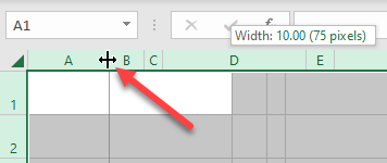
Place the cursor at the bottom edge of the row header for which you want to change the height. You will notice that the cursor would change into a plus icon
With the cursor on the bottom edge of the row header, press the left mouse key.
Keep the mouse key pressed and drag it down to increase the row height (or drag it up to decrease the row height)
Leave the mouse key when done

This is an easy way to change the row height in Excel and is a good method if you only have to do it for one row or a couple of rows.

You can also do this for multiple rows. Just select all the rows for which you want to increase/decrease the height and use the cursor and drag (for any of the selected rows).

One drawback of this method is that it doesn’t give consistent results every time you change the row height. For example, if you change the row height for one row and then again for another row it may not be the same (it may be close but may not exactly be the same)

Let’s look at more methods that are more precise and can be used when you have to change the row height of multiple rows in one go.

Also read: How to Copy Column Widths in Excel (Shortcut)

Using the Mouse Double Click Method

If you want Excel to automatically adjust the row height in such a way that the text nicely fits within the cell, this is the fastest and the easiest method.

Suppose you have a data set as shown below, and you want to change the row height of the third row (so that the entire text is visible in the row).

Below are the steps to automatically adjust the row height using mouse double-click:

Place the cursor at the bottom edge of the row header for which you want to change the height. You will notice that the cursor would change into a plus icon
With the cursor on the bottom edge of the row alphabet, double click (press the left mouse key in quick succession)
Leave the mouse key when done

When you double-click the mouse key, it automatically expands or contracts the row height to make sure that it is enough to display all the text within the cell.

You can also do this for a range of cells.

For example, if you have multiple cells and you need to at just the row height for all the cells, select the row header for these cells and double click on the edge of any of the rows.

Manually Setting the Row Height

You can specify the exact row height you want for a row (or multiple rows).

Let’s say you have a data set as shown below and you want to increase the row height of all the rows in the data set.

Below are the steps to do this:

Select all the rows by clicking and dragging on the row headers (or select the cells in a column for all the rows for which you want to change the height)
Click the Home tab
in the Cells group, click on the Format option
In the dropdown, click on the Row Height option.
In the Row Height dialog box, enter the height that you want for each of these selected rows. For this example, I would go with 50.
Click on OK

The above steps would change the row height of all the selected rows to 50 (the default row height on my system was 14.4)

While you can use the previously covered mouse double click method as well, the difference with this method is that all your rows are of the same height (which some people find better)

Keyboard Shortcut To Specify the Row Height

If you prefer using a keyboard shortcut instead, this method is for you.

Below is the keyboard shortcut that will open the row height dialog box where you can manually insert the row height value that you want

ALT + H + O + H (press one after the other)

Let’s say you have a data set as shown below and you want to increase the row height of all the rows in the data set.

Below are the steps to use this keyboard shortcut to change the row height:

Select the cells in a column for all the rows for which you want to change the height
Use the keyboard shortcut – ALT + H + O + H
In the Row Height dialog box that opens, enter the height that you want for each of these selected rows. For this example, I would go with 50.
Click on OK

A lot of people prefer this method as you don’t have to leave your keyboard to change the row height (if you have a certain height value in mind that you want to apply for all the selected cells).

While this may look like a long keyboard shortcut, if you get used to it, it’s faster than the other methods covered above.

Autofit Rows

Most of the methods covered so far are dependent on the user specifying the row height (either by clicking and dragging or by entering the value of the row height in the dialog box).

But in many cases, you don’t want to manually do this.

Sometimes you just need to make sure that the row height adjusts to make sure that the text is visible.

This is where you can use the autofit feature.

Suppose you have a data set as shown below where there is more text in each cell and the additional text is being cut off because the height of the cell is not enough.

Below are the steps to use autofit to increase the row height to fit the text in it:

Select the rows that you want to autofit
Click the Home tab
In the Cells group, click on the Format option. Doing this will show an additional dropdown of options
Click on the Autofit Row Height option

The above steps would change the row height and auto fit the text in such a way that all the text in these rows would now be visible.

In case you change the column height, the row height would automatically adjust to make sure that there are no extra spaces within the row.

There are more ways to use autofit in Excel, and you can read more about it here.

Can We Change the Default Row Height in Excel?

While it would be great to have an option to set the default row height, unfortunately as of writing this article, there is no way to set the default row height.

The Excel version that I’m using currently (Microsoft 365) has the default row height value of 14.4.

One of the articles I found online suggested that I can change the default font size and that would automatically change the row height.

While this does seem to work, it’s too messy (given that it only takes a few seconds to change the row height by any of the methods I’ve covered above in this tutorial)

Bottom line – there is no way to set the default row height in Excel of now.

And since it’s quite easy to change the row height and the column width, I don’t expect Excel to have this feature anytime soon (or ever).

In this tutorial, I’ve shown you 5 easy ways to quickly change the row height (by using the mouse, a keyboard shortcut, or by using the autofit feature).

All the methods covered here can also be used to change the column width as well.

I hope you found this tutorial useful.

Other Excel Tutorials you may like:

How to Delete All Hidden Rows and Columns in Excel
How to Indent in Excel
How to Wrap Text in Excel (with a shortcut, One Click, and a Formula)
Insert a Blank Row after Every Row in Excel (or Every Nth Row)
Delete Rows Based on a Cell Value (or Condition) in Excel
How to Lock Row Height & Column Width in Excel

Источник

In this tutorial, you will learn how to make all rows the same height and all columns the same width in Excel and Google Sheets.

When working in Excel, we often have data exported from some other system and the general layout can be pretty messy. Therefore we may need to sort out the worksheet to be able to work with data. One thing that often needs to be done is to set all rows to the same height and all columns to the same width.

Make All Rows the Same Height

To make all rows the same height, follow these steps:

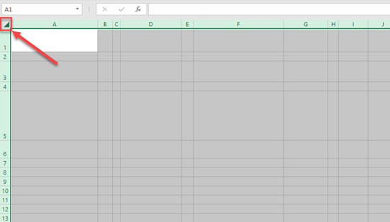
1. Select all cells in the worksheet. To do this, click on the arrow in the upper left corner of the gridlines.

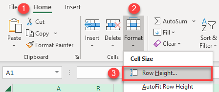
2. In the Ribbon, go to Home > Format > Row Height.

3. In the pop-up screen, (1) set Row height (for example, we set 20 here), and (2) click OK

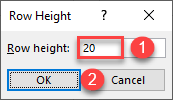
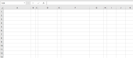
As a result, all cells in the worksheet now have the same height (20).

Make All Columns the Same Width

Similarly, we can make all columns the same width by following these steps:

1. Select all cells in the worksheet. To do this, click on the arrow in the upper left corner of the gridlines.

2. In the Ribbon, go to Home > Format > Column Width.

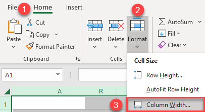
3. In the pop-up screen, (1) set Column width (for example, we set 15 here), and (2) click OK.

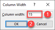
As a result, all cells in the worksheet now have the same height (15). Now the whole worksheet has cells with the same height and width.

Make All Rows the Same Height by Dragging

Another way to make all rows the same height is to drag a row boundary while all rows are selected.

1. Select all cells in the worksheet. To do this, click on the arrow in the upper left corner of the gridlines.

2. Now, click on the line between any two rows’ numbers and drag the cursor up or down to resize a row. This resizing will actually resize all the rows in the worksheet. While we’re dragging the cursor, we’ll see row heights in points and pixels, so we can set an exact value if we want.

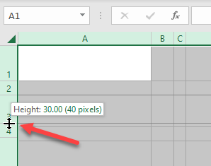
As you can see in the picture below, we set the same row height for all rows in the sheet.

Make All Columns the Same Width by Dragging

Just like sizing rows, as shown above, we can also make all columns the same width by dragging the cursor right or left.

1. Select all cells in the worksheet. To do this, click on the arrow in the upper left corner of the gridlines.

2. Now, click on the line between any column letter and drag the cursor left or right in order to resize a column. As we saw previously, this resizing will affect all the columns in the worksheet. While we’re dragging the cursor, we’ll see columns width in points and pixels, so we can set an exact value if we want.

Again, we achieved the same result and made all the columns the same width.

Note that macros can also be used to change row height and column width.

Make All Rows the Same Height in Google Sheets

To make all rows the same height in Google Sheets, do the following:

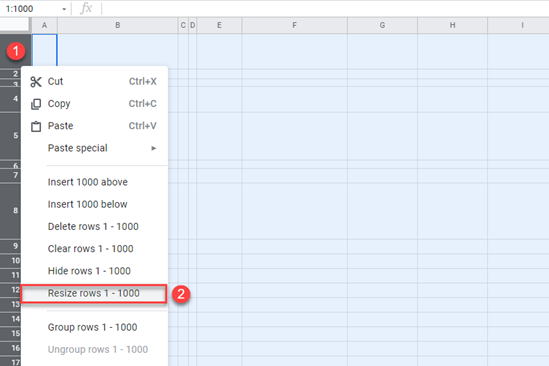
1. First, select Row 1 by clicking on its header and press CTRL + SHIFT + DOWN to select all visible rows.

2. Next, (1) click on any row heading (numbers) and (2) press Resize rows 1-1000.

3. In the pop-up screen, (1) select Specify row height and (2) set row height, for example, 25. (3) Click OK.

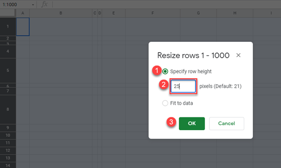
As a result, all cells have the same height (25).

Make All Columns the Same Width in Google Sheets

Now we can also make all columns the same width in Google Sheets.

1. First, select Column A by clicking on its header and press CTRL + SHIFT + RIGHT in order to select all visible columns.

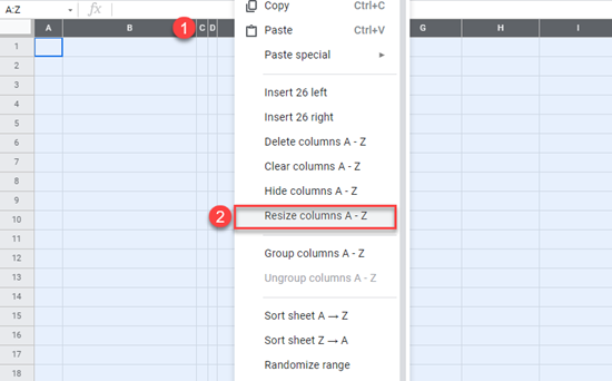
2. Next, (1) click on any column heading (letter) and (2) press Resize columns A-Z.

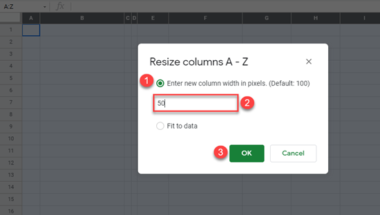
3. In the pop-up screen, (1) select Enter new column width in pixels and (2) set column width, for example, 50. (3) Click OK.

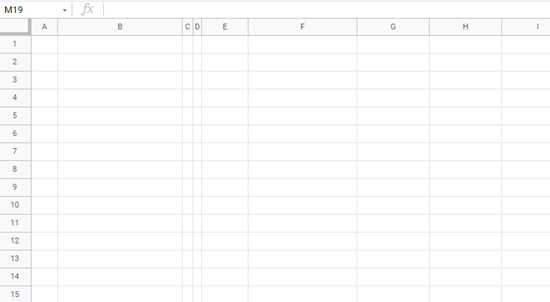
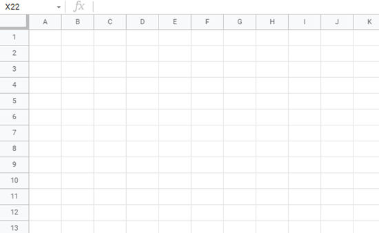
Finally, all cells in this sheet have the same height and width.

We can also resize all rows or columns in Google Sheets by dragging. This works exactly the same as shown above for Excel.

Источник

Set a column to a specific width

Set a column to a specific width

See Also

Change the column width or row height in Excel

Resize rows

Resize columns

Automatically resize all columns and rows to fit the data

Need more help?

See Also

Need more help?

Want more options?

Начнём с теории

Спрашиваем высоту ряда

Немного практики

Разбираемся со вставкой/удалением рядов

Выводы

Change the Row Height with Click and Drag (Using the Mouse)

Using the Mouse Double Click Method

Manually Setting the Row Height

Keyboard Shortcut To Specify the Row Height

Autofit Rows

Can We Change the Default Row Height in Excel?

Make All Rows the Same Height

Make All Columns the Same Width

Make All Rows the Same Height by Dragging

Make All Columns the Same Width by Dragging

Make All Rows the Same Height in Google Sheets

Make All Columns the Same Width in Google Sheets