
Numbering in Excel means providing a cell with numbers like serial numbers to some table. We can also do it manually by filling the first two cells with numbers and dragging them down to the end of the table, which Excel will automatically load the series. Else, we can use the =ROW() formula to insert a row number as the serial number in the data or table.
When working with Excel, some small tasks need to be done repeatedly. However, if we know the right way to do it, they can save a lot of time. For example, generating the numbers in Excel is a task that is often used while working. Serial numbers play a very important role in Excel. It defines a unique identity for each record of your data.
One of the ways is to add the serial numbers manually in Excel. But it can be a pain if you have the data of hundreds or thousands of rows and must enter the row number for them.
This article will cover the different ways to do it.
Table of contents
- Numbering in Excel
- How to Add Serial Number in Excel Automatically?
- #1 – Using Fill Handle
- #2 – Using Fill Series
- #3 – Using the ROW Function
- Things to Remember about Numbering in Excel
- Recommended Articles
How to Add Serial Number in Excel Automatically?
There are many ways to generate the number of rows in Excel.
You can download this Numbering in Excel Template here – Numbering in Excel Template
- Using Fill Handle
- Using Fill Series
- Using ROW Function
#1 – Using Fill Handle
It identifies a pattern from a few already filled cells and then quickly uses that pattern to fill the entire column.
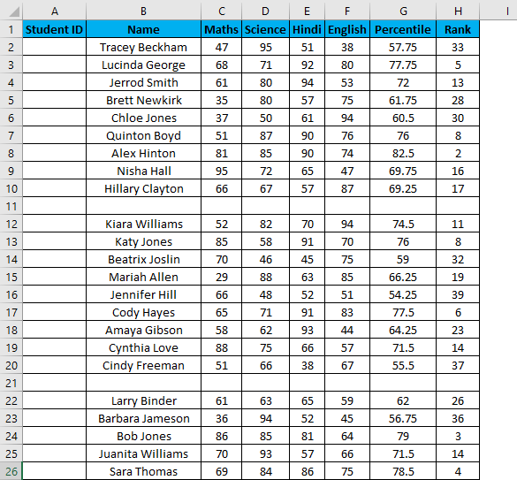
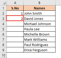
For example, let us take the below dataset.
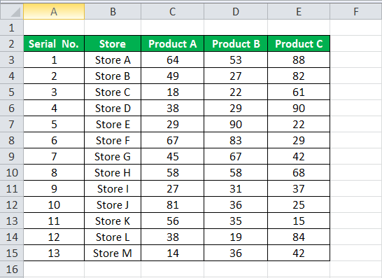
For the above dataset, we have to fill the serial no record-wise. Follow the below steps:
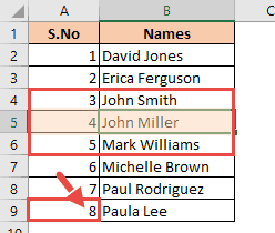
- First, we must enter 1 in cell A3 and insert 2 in cell A4.
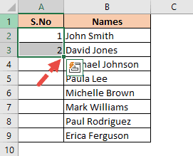
- Then, select both the cells as per the below screenshot.

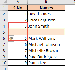
As we can see, a small square is shown in the above screenshot, which is rounded by a red color called “Fill Handle” in Excel.
Place the mouse cursor on this square and double-click on the fill handle.
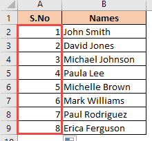
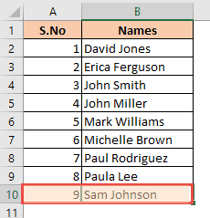
- It will automatically fill all the cells until the end of the dataset. For example, refer to the below screenshot.

As the fill handle identifies the pattern, fill the individual cells with that pattern.
If you have any blank row in the dataset, the fill handle would only work until the last contiguous non-blank row.

#2 – Using Fill Series
It gives more control over data on how the serial numbers are entered into Excel.
For example, suppose you have below the score of students subject-wise.

Follow the below steps to fill series in the Excel:
- We must first insert 1 in cell A3.
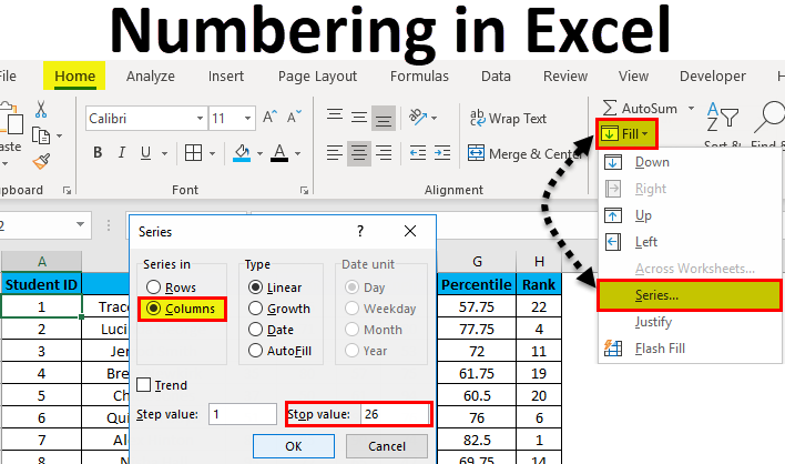
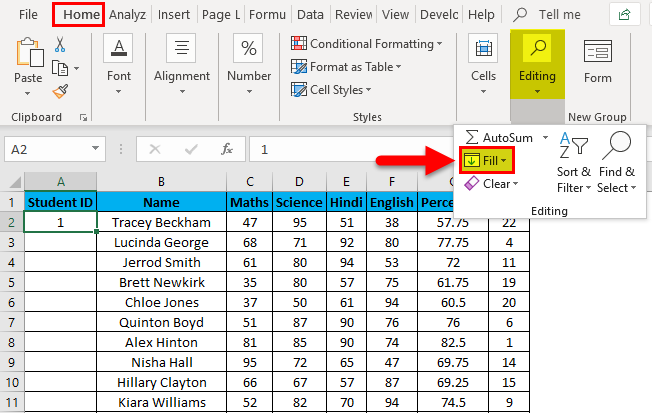
- Then, go to the “HOME” tab. Next, click on the “Fill” option under the “Editing” section, as shown in the below screenshot.

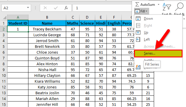
- Click on the “Fill” dropdown. It has many options. Click on “Series,” as shown in the below screenshot.

- It will open a dialog box, as shown below screenshot.

- Click on “Columns” under the “Series in” section. Then, refer to the below screenshot.

- Insert the value under the “Stop value” field. In this case, we have 10 records; enter 10. If we skip this value, the Fill “Series” option may not work.
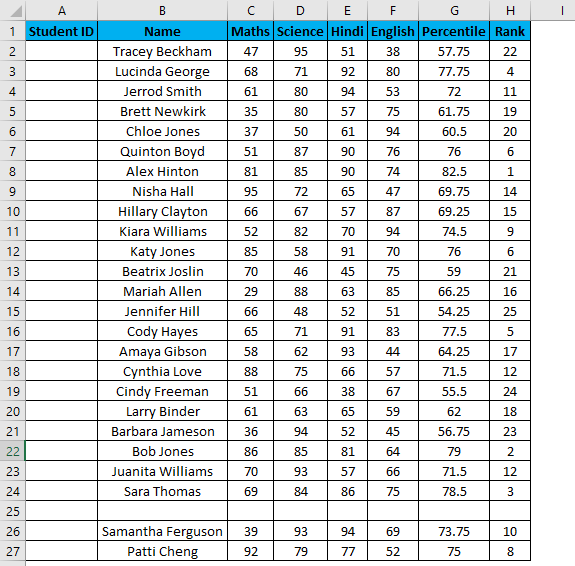
- Enter “OK.” It will fill rows with serial numbers from 1 to 10. Refer to the below screenshot.

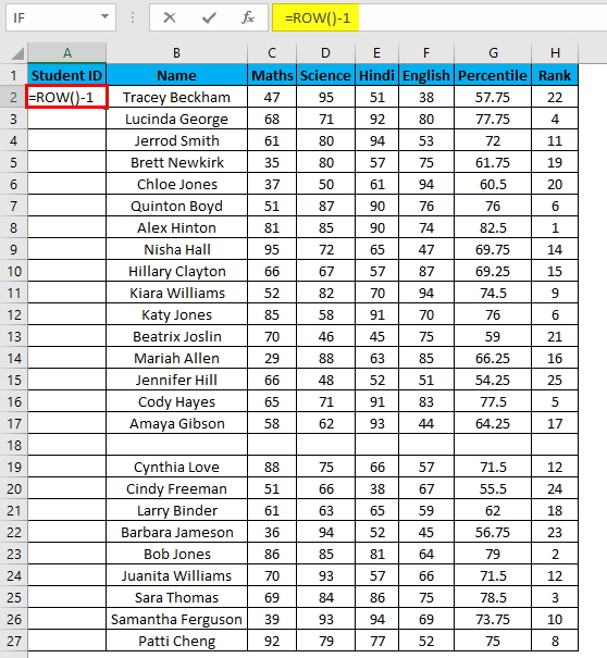
#3 – Using the ROW Function
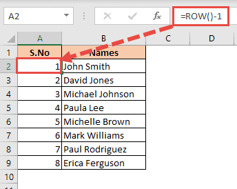
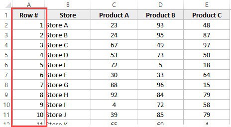
Excel has a built-in function, which also can be used to number the rows in Excel. To get the Excel row numbering, we must enter the following formula in the first cell shown below:

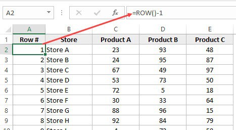
- The ROW function gives the Excel row number of the current row. We have subtracted 3 from it as we started the data from the 4th. If the data starts from the 2nd row, we must remove 1 from it.
- See the below screenshot. Using =ROW()-3 formula.

Drag this formula for the rest of the rows. The final result is shown below.
Using this formula for numbering will not damage the numbers if we delete a record in the dataset. Furthermore, since the ROW function does not reference cell addresses, it will automatically adjust to give the correct row number.
Things to Remember about Numbering in Excel
- The “Fill Handle” and “Fill Series” options are static. Therefore, if we move or delete any record or row in the dataset, the row number will not change accordingly.
- The ROW function gives the exact numbering if we cut and copy the data in Excel.
Recommended Articles
This article is a guide to Numbering in Excel. We discuss how to automatically add serial numbers in Excel using the fill handle, fill series, and ROW function, along with examples and downloadable templates. You may learn more about Excel functions from the following articles: –
- Auto Numbering in ExcelThere are two approaches for auto numbering. To begin, fill the first two cells with the series you wish to insert and drag it to the table’s end. Second, use the =ROW() formula to get the number, and then drag it to the table’s end.read more
- Row Limit in Excel
- Excel Negative NumberIn Excel, negative numbers, i.e. numbers less than 0 in value, are displayed with minus symbols by default.read more
- IsNumber FunctionISNUMBER function in excel is an information function that checks if the referred cell value is numeric or non-numeric.read more
- Null in ExcelNull is a type of error in Excel that occurs when two or more cell references provided in formulas are wrong, or when their position is incorrect. Using space in formulas between two cell references, for example, will result in a null error.read more
Reader Interactions
If you’re working with large sets of data in Excel, then it’s a good idea to add a serial number, row number or ID column to the data.
A serial number is a unique identifier for a row or record of data and they will usually start at 1 and increase incrementally with each row.
This way you can refer to each record in your data set by the serial number.
In this post, I’ll show you 15 interesting ways which you can add row numbers to your data.
Use the Row Headings
Good news! Excel comes with serial numbers out of the box.
On the very left hand side of every sheet is the row heading with row numbers in an incrementally increasing sequence.
You can use these as serial numbers for your data.
Pros
- You don’t need to do anything to create them as they are there by default.
- These numbers will adjust when you delete or insert a row.
- Works inside Excel Tables.
Cons
- You can’t change them.
- You need to position your data starting in cell A1.
- If your data contains column headings, then the row number will start at row 2 for the first record.
Use the Fill Handle
This one is an amazing trick!
Once you learn it, there is no going back to the old way of manually typing each number of a sequence.
The fill handle will automatically create a sequence of serial numbers for you with just a click and drag.
You first need to enter two sequential numbers.
Notice the active cell has a square in the lower right?
This is the Fill Handle and you can use it to automatically fill in the rest of the sequence which you started to add manually.
Select the first two cells and then hover your mouse cursor over the lower right corner until it turns into a small black plus sign. Then click and drag down to the end of your data.
If you’re working with a large data set, then click and drag might not be feasible. In this situation, you can double click on the fill handle to fill the sequence down to the end.
When you release the fill handle this will fill in the sequence of numbers and a small fill handle options menu will appear at the bottom right of your filled sequence.
There is one handy option in this menu that allows you to avoid filling down any cell formatting.
Click on the menu options and choose Fill Without Formatting and any copied cell formatting will be removed.
Pros
- Easy to use and only requires manually entering two values.
- The serial number entered in a row will not change once it’s entered.
- Deleting or inserting a row won’t affect other record ID’s.
- Works inside Excel Tables.
Cons
- Each time you add new rows to the bottom of your data table you will need to manually add a serial number or repeat the fill handle process.
- For large data sets, clicking and dragging the fill handle to the end can be tedious.
Use the Fill Series Command
This option is very similar to the fill handle method, but doesn’t require and long click and drag actions down the length of your data.
Add the first two serial numbers to your data set. Then select the entire range of cells which you would like to fill including the two serial numbers you have already entered.
To select a longer range, it’s easier to start at the bottom and select up to the top.
If you place the active cell cursor in the next column which contains data, you can use Ctrl + Down to get to the last cell. Move the cursor back over to the ID column, then Use Ctrl + Shift + Up to select all the blank ID cells. Then use Shift + Up to select any previously entered serial number cells.
Go to the Home tab of the ribbon and click on the Fill command then choose Series.
This will open the Series menu.
- Choose Columns for the Series in option.
- Choose AutoFill for the Type option.
- Press the OK button.
This will fill in the remaining series in your selected blank cells.
Pros
- Easy to use and only requires entering the first two numbers manually.
- No long click and drag actions required.
- You can delete or insert rows without affecting other existing serial numbers.
- Works inside Excel Tables.
Cons
- This is not a dynamic solution, so when you add new rows to your data table you will need to manually add a serial number or repeat the fill process.
Add One to the Previous Number
This is the intuitive method to adding a series of numbers to your data. Excel’s is designed to calculate, so adding 1 to the previous serial number is no problem.
= B3 + 1Enter the value 1 into the first row of your data. Then in the next row enter the above formula. In this example B3 is the cell directly above.
Now you can copy and paste this formula down the remaining rows. To do this quickly, double click on the fill handle of the cell which contains the formula.
Pros
- Easy to implement.
- Easy for someone to understand what the formula is doing.
- You can copy and paste the formula down when new rows are added.
Cons
- If you delete any row, you will get #REF! errors for all rows below as you are deleting a cell that is referenced by those cells below.
- The formula is not consistent for the entire column since the first row needs to contain a hard coded value of 1.
Use a Relative Reference Named Range
This method is going to use the same idea where you add 1 to the previous serial number, but it is going use a clever trick to make it more robust.
What you need to do is create a named range that will always refer to the cell above it.
Then you can reference this named range instead of a direct cell address like B3.
Go to the Formulas tab and click on Define Name.
This will open the New Name menu. Give your named range a name like Above, this is how you will reference it inside formulas later.
= INDIRECT ( "R[-1]C", FALSE )Add the above formula in the Refers to section of the New Name menu then press the OK button.
This formula uses the INDIRECT function with row and column notation. R[-1] indicates the reference is one row above the current cell.
Now when you use the Above name inside a formula it will reference the cell directly above the cell which you are entering the formula.
= SUM ( Above, 1 )Enter the above formula into the first row and then copy and paste it to the end of your data.
Using the SUM function is a small improvement to the previous method as there is no need to enter a value in the first row. The formula can be applied consistently for each row.
The SUM function will count text values as zero, so you can safely reference the column headings when the formula is in the first row without producing a #VALUE! error.
Pros
- You can copy and paste the formula down when new rows are added.
- Use the same formula for the entire row.
- Works well inside Excel tables.
- Serial numbers will dynamically adjust when you delete or insert a row.
Cons
- Takes more time to set up.
- The formula might not be as obvious to someone else looking at your spreadsheet,
- The named range uses the INDIRECT function which is a volatile Excel function. They can slow down your Excel workbook because they are recalculated more frequently.
Use the ROW Function
There is an Excel function that can return the current row number and it’s perfect for creating serial numbers.
= ROW ( ) - ROW ( $B$2 )Add the above formula, where B2 refers to the column heading cell, into the first row and copy and paste it down.
The ROW function returns the row number of the current row when no argument is passed to it. In order to start the serial numbers at 1, we then need to subtract off the row number of the column heading cell. This is accomplished using an absolute reference to the cell with the column heading.
Pros
- Easy to implement.
- Inserting or deleting a row won’t cause any errors and serial numbers will update accordingly.
- Works inside Excel Tables.
Cons
- The formula needs to reference the column heading cell with an absolute reference.
Use the COUNTA Function
This is another formula option that will rely on counting previous rows of data.
In order to use this formula, you will need a column that will never contain blank values as the COUNTA function does not count empty cells.
= COUNTA ( $C$3:C3 )Enter the above formula into the first row and then copy and paste it to the end of your data. In this formula C3 is a cell in the first row but another column which will not contain any blank values.
Notice the range reference in the formula contains a partial absolute reference with the $ symbol. This causes the formula to include all records above the current record in its count as it gets copied down the data set.
Pros
- Easy to implement where the only tricky part is adding the partial absolute reference.
- You can insert or delete rows without errors.
- Works with Excel Tables.
Cons
- You need to refer to another column which can’t have any blank values.
Use the SUBTOTAL Function
The SUBTOTAL function is interesting because it can return values based on what cells are visible.
It can also be used to perform other aggregations like a count and not just a sum.
This means you can use it to create serial numbers that change based on filtered data.
= SUBTOTAL ( 3, $C$3:C3 )Add the above formula into the first row then copy and paste it down the data.
This formula works exactly like the COUNTA method, because it is the same. The first argument in the SUBTOTAL function tells Excel to use a count type aggregation.
The only difference is when you filter your data, the serial numbers will update based on what is still visible.
Pros
- Same pros as COUNTA method.
- You can use filters on your data and they will dynamically change the serial numbers.
Cons
- Same cons as COUNTA method.
- The SUBTOTAL function is less known by most Excel users.
Use the SEQUENCE Function
The SEQUENCE function is a new dynamic array function. This means one formula can produce an array of values.
It can do a lot more, but this function can also generate a single column of increasing numbers that start at 1. Perfect for serial numbers!
= SEQUENCE ( COUNTA ( C3:C8 ) )Add the above formula into the first row of data. In this example C3:C8 is the entire range of a column. This will determine how many serial numbers the SEQUENCE function will return.
= SEQUENCE ( 6 )Another approach is to hard code the row count inside your SEQUENCE function like the above formula. Unfortunately, this method would mean you need to manually adjust the count each time you add or remove rows of data.
Pros
- You only need one formula. No need to copy and paste a formula down to the end of your data set.
- Inserting or deleting any row other than the first one won’t produce any errors and your serial numbers will adjust accordingly.
Cons
- Deleting the first row will delete all the serial numbers.
- Can’t be used inside Excel Tables.
- If you add rows at the bottom of your data set, you will need to adjust the range reference in the SEQUENCE function to include these.
- The COUNTA function will require non blank values.
Use Power Pivot
This one is a bit weird since it will create serial numbers inside a pivot table.
But it may be just what you’re lookin for.
You can use power pivot with a calculated column to number your pivot table rows.
Select your table of data and go to the Power Pivot tab and click on Add to Data Model.
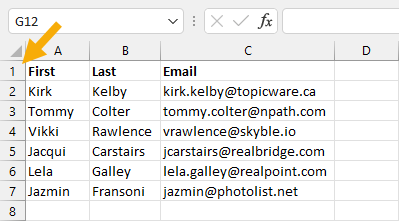
= RANK.EQ( Data[Email], Data[Email], ASC )This will open the power pivot add-in and you’ll be able to add the above formula into the table.
In this example, the table has been named Data and we are ranking the Email column which contains unique text values. This results in column that can be used as a serial number.
To use this calculated column inside a pivot table.
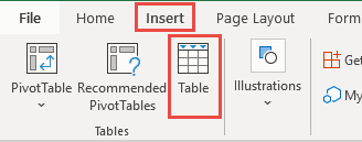
- Go to the Insert tab.
- Click on PivotTable.
- Choose From Data Model from the options.
- Choose the location you would like to place the pivot table.
- Add add the fields into the Rows area of your new pivot table including the Rank calculated column.
- Go to the Design tab ➜ Report Layout ➜ Show in Tabular Form. This will make it look more like a dataset instead of a pivot table.
Pros
- You can create serial numbers inside a pivot table.
Cons
- You need a column with unique values like an email.
- Results are not ordered.
Use VBA Code
VBA has been in Excel and other Office applications for a long time.
It was the go to method for automating any task in Excel. So you can certainly use it to automatically generate your serial numbers.
These days, there are usually much better options available and I would only recommend using a VBA solution as a last resort.
Sub AddSerial()

Dim cell As Object
Dim count As Integer
count = 0

For Each cell In Selection
    count = count + 1
    cell.Value = count
Next cell

End Sub
Add the above code into the visual basic editor.
- Pres Alt + F11 to open up the visual basic editor.
- Right click inside the VBAProject window.
- Select Insert from the menu.
- Select Module from the submenu.
- Paste the code into the module.
The above code will add an increasing sequence of numbers starting at 1 into any selected range.
Now you can run the code.
- Select the entire column which you want to add serial number into.
- Press Alt + F8 to open the Macro dialog box.
- Select the macro to run.
- Press the Run button.
This will fill your selected range with a sequence of numbers starting at 1.
Pros
- Adds static numbers into any range.
Cons
- Uses VBA and will require the workbook to be saved as an xlsm file.
- Hard to set up and run.
- You will need to re-run the code if you add or insert rows to your data set.
Use an Index Column in Power Query
Power Query is an amazing data transformation tool found in Excel and other Microsoft products.
If you’re already using it to import your data from an external source into Excel, then it might be the perfect solution to adding serial number to your data.
If your data is already in Excel, you can still use power query to add serial numbers but you will need to add your data into an Excel table first.
I wrote a detailed article about Excel Tables, where you can learn all about them including how to convert your data into a table.
Add your data into query by using a From Sheet query. Select a cell inside your table ➜ go to the Data tab ➜ choose From Sheet.
This will open up the power query editor and you will be able to add a column with serial numbers from here.
Go to the Add Column tab and click on the Index Column command. Click on the small arrow icon of the Index Column button to choose to start the index From 1.
Now you can go to the Home tab ➜ Close & Load ➜ Close & Load To ➜ Choose to load the results into an Excel table and pick the location to load it to.
Your data will be loaded into another table with an extra index column.
If you add or remove data from the source, you will need to refresh the query output to see the updated results. You can refresh the query by right clicking on the table and choosing Refresh from the menu options.
Pros
- Great option if you’re using power query to import your data from an external source already.
- Easy to refresh once it is set up.
Cons
- Power query can be intimidating to someone using it for the first time.
- It doesn’t add the serial numbers into the data source, it will only add them to the output of a query on the data source.
Use the Connection Properties for Connected Tables
If your data has been loaded into a table from an external source like power query or an exported SharePoint list, then you can enable row numbers from the connection properties menu.
Select your connected table and go to the Data tab and click on the Properties command.
This will open the External Data Properties menu and you can enable the option to Include row numbers and press the OK button.
Now you need to refresh the connection in order to see the row numbers. Go to the Data tab and click on the Refresh button.
After refreshing the connection, you will see a new column in the table called _RowNum which starts the count at 0.
Pros
- You can delete or insert rows in the source data and the row number will update when you refresh the connection.
Cons
- This feature only works with connected data tables.
- The row numbers setting is hard to discover.
- The row number column can only appear as the very left column in the table.
- The row numbers start at 0 and can’t be changed to start at 1 instead.
- The column heading for your serial numbers can’t be changed from _RowNum.
Use Office Scripts
Office Scripts is a new TypeScript based scripting language which is currently only available in Excel online for Enterprise Microsoft 365 plans.
This is the replacement for VBA and you can certainly use it to auto generate a set of row numbers.
You will need a few things in order to use this method first.
- Your Excel file has to be saved in SharePoint.
- You need to open your Excel file in the Excel web application.
- You need to be on an enterprise level Microsoft 365 plan.
- The Office Scripts feature needs to be enabled by your IT admin.
Open your file in Excel online then go to the Automate tab and click on New Script.
function main(workbook: ExcelScript.Workbook) {
	let selectedSheet = workbook.getActiveWorksheet();
	let myID = selectedSheet.getRange("Data[ID]");
	let myCellCount = myID.getCellCount();
	let mySerialNumbers = new Array(Array(myCellCount));
	for (var i = 0; i < myCellCount; i++) {
		mySerialNumbers[i] = [i+1]
	}
	selectedSheet.getRange("Data[ID]").setValues(mySerialNumbers);
}
Paste in the above code into the Code Editor. You can rename the script and press Save Script to save the script.
Press the Run button in the Code Editor to run the script.
This script relies on your data being inside an Excel Table named Data with a column named ID.
Pros
- Once this is set up, its very easy to use.
Cons
- Excel file needs to be saved in SharePoint.
- Office Scripts are only available in Excel online for Enterprise Microsoft 365 plans.
- You can only run this script from Excel online.
Use Power Automate
Now that you have an Office Script to add serial numbers to Excel, you can use Power Automate to automate the running of this script.
You can use power automate to run this script on a schedule, so you can automatically update your serial numbers every day or even every hour.
- Log into https://flow.microsoft.com/
- Click on Create in the left hand navigation pane.
- Click on Scheduled cloud flow.
- Give your flow a name like Add Serial Numbers.
- Set the start date to today’s date and time.
- Set the frequency which you would like the flow to run.
- Click on the Create button.
Now add a Run script step to the flow and select the file and script to run then Save the flow.
This will now automatically run the script to add serial number at your desired frequency.
Pros
- The solution automatically runs in the background.
- You can work on the file in the desktop or web app while the flow runs.
Cons
- Requires a complex setup.
- Needs Microsoft 365, SharePoint and Office Scripts.
Conclusion
There are a ton of options when it comes to adding serial numbers to your data in Excel.
Each method will have various pros and cons that might make them a better option for your use case. It’s worth exploring them all to see which will work best for you.
Whatever your skill set there is an option for you that will get you your desired results.
Did I miss your favourite way to add row numbers in this post? Let me know in the comments if you have another method you use!
About the Author
John is a Microsoft MVP and qualified actuary with over 15 years of experience. He has worked in a variety of industries, including insurance, ad tech, and most recently Power Platform consulting. He is a keen problem solver and has a passion for using technology to make businesses more efficient.
Excel Numbering (Table of Contents)
- Numbering in Excel
- How to Add Serial Number in Excel?
Numbering in Excel
There are various ways of numbering in excel, which are Fill Handle, Fill Series, Row Function mainly. By Fill Handle, we can drag already written 2-3 numbers in sequence until the limit we want. By Fill Series, which is available in the Home menu tab and select the Series option, select the lowest and highest numbers. And if we select the Row function for numbering, then also we can create a number in the sequence.
How to Add Serial Number in Excel?
To add a serial number in Excel is very simple and easy. Let’s understand the working of adding a serial number in Excel by some methods with its example.
You can download this Numbering Excel Template here – Numbering Excel Template
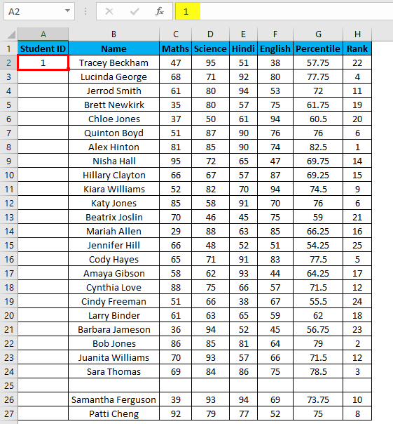
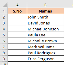
Example #1 – Fill Handle Method
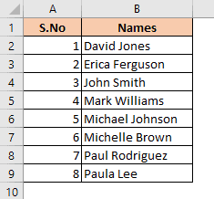
Suppose you have the following dataset. And you have to give a Student ID to each entry. Student ID there will be the same as a serial number of each row entry.
You can use the fill handle method here.
For example, you want to give Student ID 1056 to the first student, and after it should be numerically increasing, 1056, 1057,1058, and so on…
Steps to number rows in Excel:
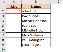
- Enter 1056 in cell A2 and 1057 in cell A3.
- Select both cells.
- Now you can notice a square at the bottom-right of selected cells.
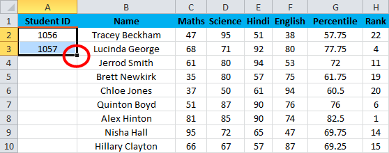
- Move your cursor to this square; now, it will be changed to the small plus sign.
- Now double click this plus icon, and it will automatically fill the series till the end of the dataset.

Key Point:
- It identifies a pattern from a few filled cells and quickly fills the entire selected column.
- It would only work till the last contiguous non-blank row. Viz. If you have any blank row(s) between your dataset. It will not detect them, so it’s not recommended to use the fill method.
Example #2 – Fill Series Method
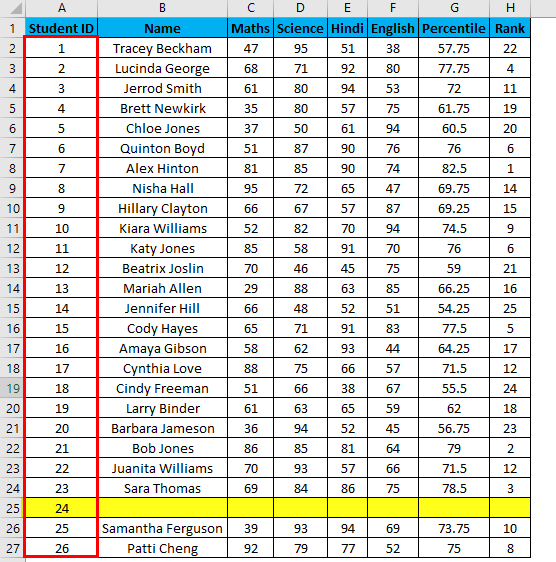
Suppose now we have the following dataset (same as above, now entries are only 26.).
Steps to use the Fill Series method:
- Enter 1 in cell A2.
- Go to the Home tab.
- In the Editing group, click on the Fill drop-down.
- From the drop-down, select Series.
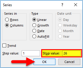
- In the Series dialog box, select Columns in the ” Series in ” option.
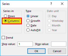
- Specify the Stop value. Here we can enter 26 and then click Ok.
- If you don’t enter any value, Fill Series will not work.
Hotkey to use fill series: ALT key+ H+ FI+ S
You can notice, it overcomes the drawback of the previous method. But then it has its own drawback that if we have blank rows in between of the dataset, Fill Series would still fill the number for that row.
Example #3 – COUNTA Function
Suppose you have the same data set as above, now if you want to number rows in excel only which are filled Viz. Overcoming the shortcomings of the above 2 methods. You can use a COUNTA function here.
Steps to use a COUNTA Function:
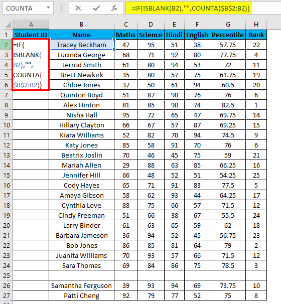
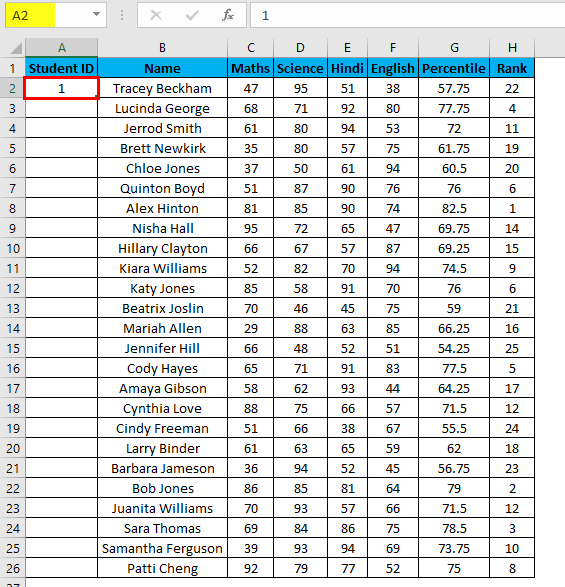
- Now enter the formula in the cell A2 i.e. =IF(ISBLANK(B2),””,COUNTA($B$2:B2))
- Drag it down till the last row of your data set.

- In the above formula, the IF function will check if cell B2 is empty or not. If found empty, it returns a blank, but it returns the count of all the filled cells till that cell if it’s not.
Example #4 – Increment Previous Row Number
This is a very simple method. The main method is to add 1 to the previous row number simply.
Suppose you again have the same dataset.
- In the first row, manually enter 1 or any number from where you want to start numbering all rows in excel. In our case. Enter 1 in cell A2.
- Now in cell A3, simply enter the formula=A2+1.
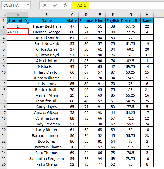
- Drag this formula until the last row, and it will be increased by 1 in each following row.

Example #5 – Row Function
We can even use a row function to give serial numbers to rows in our columns. In above all methods, the serial number inserted is fixed values. But what if a row is moved or you cut and paste data somewhere else in the worksheet?
The above problem can be resolved by using the ROW function. To number the rows in a given dataset using the ROW function.
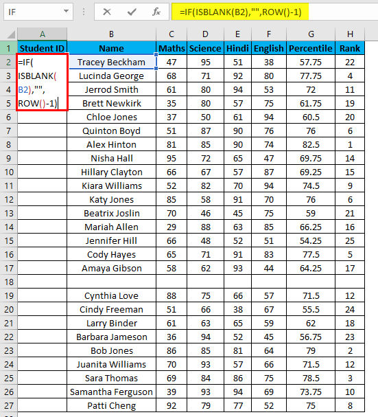
- Enter the formula in the first cell i.e. =IF(ISBLANK(B2),””,ROW()-1)
- Drag this formula until the last row.
- In the above formula IF function will check if the adjacent cell B is blank or not. If it’s found blank, it will return space, and if non-blank, then row function will come into the picture. ROW() function will give us the row number since the first row in Excel consists of our dataset. So we don’t need to count it. To eliminate the first row, I have subtracted 1 from the returned value of the above function.
- But it will not still adjust the row number, and a blank row will still have a serial number assigned to it. Though it is not shown, look at the below screenshot.
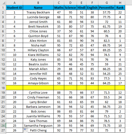
- You can overcome the above issue with this formula, i.e.=ROW()-1
- Drag this formula until the last row.
- But now, it will consider the blank rows in the dataset and will number them as well. Consider the below screenshot.

The main advantage of using this method is even if you delete one or more entries in your dataset. You don’t need to struggle with the numbering of rows each and every time, and it will be corrected automatically in excel.
So by now, I have discussed 5 unique methods to give serial numbers to row in a dataset stored in Excel. Although there are numerous methods to do the same, above five are the most common and easy to use method which can be implemented in different scenarios.
Things to Remember About Numbering in Excel
- While storing data in Excel, we often need to give serial numbers to each row in our data set.
- Entering a serial number to each and every row in the huge dataset can be time-consuming and prone to error.
Recommended Articles
This has been a guide to Numbering in Excel. Here we discuss how to add serial Numbers using different methods in excel along with practical examples and a downloadable excel template. You can also go through our other suggested articles –
- ISNUMBER Excel Function
- Negative Numbers in Excel
- Excel ISNUMBER Formula
- VBA Number Format
Wondering how to add serial number in Excel in simple ways? Read the article to know.
Serial numbers are as important in data as salt in food. You never feel their presence but their absence makes your data tasteless. It is always important to add serial numbers to your data and one can do it in many ways in Excel.
Adding serial numbers to Excel requires you to follow a few steps. Before we jump into it, let us looks at an alternative to Excel that does the same work in simpler and lesser steps.
When it comes to adding serial numbers in Lio, you really do not have to do ANYTHING. When you create a new sheet/document on the app, it automatically comes with serial numbers.
Lio makes your work very easy taking care of all the nitty-gritty of a document without you having to do much or in this case absolutely nothing.
Simple Steps To Add Serial Number In Excel
Let us learn how to add serial numbers in Excel.
Row Numbers as Serial Numbers
In a spreadsheet, you have row numbers that act as serial numbers for the data.
If you don’t want to use serial numbers for filtering or any other purpose then you can use the row headers.
Else you can follow the below-mentioned methods and add serial numbers.
Fill Series To Automatically Add Serial Numbers
Now let’s say you want to automatically number rows up to 10000 or 100000 and you want to do this in one go.
Use fill series to generate a column with serial numbers.
Here are the steps.
- Select the cell from where you want to start your serial numbers and insert “1” in it.
- Now, go to the home tab ➜ editing ➜ fill ➜ series.
- In the series window, do the following.
- Series In = Column.
- Step Value = 1
- Stop Value = 10000 or whatever you want up to.
- Click OK.
It works like a serial number generator and can be used even if you want up to one million.
Add Roman Numbers as Serial Numbers
To add roman numbers as serial numbers, use the roman function with ROW.
Follow these simple steps:
- Enter the following formula in the cell from where you want to start.
=ROMAN(ROW())
- Drag down the formula up to the serial number you want.
Understand Your Business With Tables.
Lio brings you an easy way of creating tables in your document that would positively Effect your business.
Add a Serial Date in a Column
Let us suppose you want to enter serial-wise dates in a column, you have two different methods for this.
First, add starting date in a cell and then in the next cell downward refer to the above cell and add “1” into it.
As you know Excel stores dates as numbers and every date has a unique number.
So, when you add “1” to the date it will return the next date in the result.
The second method.
Enter the starting date into a cell and then use the fill handle to extend it to the desired date.
Just like serial numbers, you will get a sequence of dates in the column.
Use Fill Handle to Add Serial Numbers
To add serial numbers using the fill handle you can use the following steps.
- Enter 1 in a cell and 2 in the next cell downward.
- Select both the cells and drag them down with the fill handle (a small dark box at the right bottom of your selection) up to the cell where you want the last serial number.
- Once you get serial numbers up to what you want, release your mouse from the selection.
This is how easy it is to add serial numbers in Excel. You can use any method to do it. Now practice these methods to remember them.
Serial Numbers in a Table
On adding a new entry, the table automatically drag-down the formula into the new cell.
Insert a formula in the first two or two entries, and you’ll get it automatically.
In the below table when you enter a new entry in a new serial number automatically generates.
Convert Serial Numbers to Serial Dates
If you already have serial numbers in your worksheet and you want to convert them to serial dates then you can simply do that with the following formula.
Let’s say you have serial numbers starting from A1, then in cell B1, add the below formula.
=DATE(2017,1,A1)

After that, drag down it up to the last serial number cell and you’ll get a sequence of dates.
Add Serial Numbers with a VBA Code
This macro code can be useful if you want to create a series of numbers without using formulas.
Sub AddSerialNumbers()
Dim i As Integer
On Error GoTo Last
i = InputBox(“Enter Value”, “Enter Serial Numbers”)
For i = 1 To i
ActiveCell.Value = i
ActiveCell.Offset(1, 0).Activate
Next i
Last:
Exit Sub
End Sub
Get Serial Numbers with COUNTA Function
Using COUNTA is a nice way to add serial numbers to your data. By using it you can actually count your data entries and give them a number.
Follow these simple steps.
- Enter the following formula in the cell from where you want to start your serial numbers. (For example, if your first data entry starts from F1, enter the below formula in E1).
=COUNTA(F$1:F1)
- Drag down the formula up to the serial number your want.
Generate Serial Numbers by Adding One in the Previous Number
This is my favorite method and believes me, it’s lightning-fast.
Follow these steps
- Enter 1 in the cell from where you want to start your serial numbers.
- In the next down cell, enter formula =G1+1 (G1 is the starting cell here).
- Drag this formula down, up to the serial numbers you want.
Use the ROW Function to Drag Serial Numbers
ROW is an effective way to insert serial numbers in your worksheet.
It can return the row number of a reference and when you skip referring to any cell it will return the row number of the cell in which you have entered it.
Here are the simple steps.
- Go to cell A1, edit it, and enter the =ROW() formula in it.
- Now drag the formula to down, up to the serial number you want.
Dynamic Serial Numbers for Filters
Let’s say you have serial numbers in a data table and when you filter some specific data from it shows you actual serials.
But, if you use a dynamic method to insert serial numbers then you can get double benefits.
First, whenever you filter data it’ll show you the serial number according to the filtered item.
Second, if you want to paste that filtered data somewhere else, you don’t have to insert them again.
For this, you can use the SUBTOTAL function and the formula will be like below.
=SUBTOTAL(3,B$2:B2)

After that, drag this formula up to the last cell of the table. Now. whenever you filter data you’ll dynamic serial number.

Maximize Your Online Business Potential for just ₹79/month on Lio. Annual plans start at just ₹799.
How Lio can Help You
Lio is a great platform that can help entrepreneurs, homemakers, students, businessmen, managers, shop owners, and many others. This mobile application helps to organize business data and present them in an eye-catching manner.
Lio is a great platform for small business owners and can track a wholesome record of employee information for better employee management, customer data, etc. You can handle those data with ease.
If you want to be a professional, then you must save your time, you need to learn to arrange all the business strategies in one place. In that case, Lio can be your partner.
Entrepreneurs can also allow multiple authorized users of their office to access the information from various locations within minutes.
Lio is definitely for the win and using it for your business is only going to make your journey smooth and easy to track.
Step 1: Select the Language you want to work on. Lio on Android

Step 2: Create your account using your Phone Number or Email Id.

Verify the OTP and you are good to go.
Step 3: Select a template in which you want to add your data.

Add your Data with our Free Cloud Storage.
Step 4: All Done? Share and Collaborate with your contacts.


Experts know the importance of serial numbers. Serial numbers are like salt. You never feel their presence but their absence makes your data tasteless.
Yes, they are important.
Because with a serial number you can have a unique identity to each entry of your data.
But the sad news is, adding them manually is a pain. It’s really hard to add a number in every row one after another.
The good news is, there are some ways which we can use to automatically add serial numbers in a column.
14 Ways to Insert Serial Number Column in Excel
And today, in this post, I’d like to share with you 14-Quick Methods. You can use any of these methods which you think is perfect for you.
These methods can generate numbers up to a specific number or can add a running column of numbers. Choose one of the below methods as per your need and if you think you have a way, then please share it with me in the comment section.
Method #1
Method #2
Method #3 (Fastest)
Method #4
Method #5 (My Favorite ?)
Method #6
Method #7
Method #8 (VBA Code)
Method #9
Method #10
Method #11
Method #12 (For Pivot Table Lovers)
Method #13
Method #14
Conclusion
If you have data whether small or large it is must to add serial numbers to it. The one thing which you really need to understand that a serial number give a unique identity to each entry.
And, with all the methods you have learned above it’s no big deal to create a serial number column in the data, no matter which situation you are in.
I hope you found this useful, but now, tell me one thing.
Which method do you prefer to insert serial numbers?
Please share your views with me in the comment section. I’d love to hear from you and please don’t forget to share it with your friends, I am sure they will appreciate it.
More Tutorials
- Convert Negative Number into Positive in Excel
- Insert (Type) Degree Symbol in Excel
- Convert a Formula to Value in Excel
- Insert a Timestamp in Excel
- Insert Bullet Points in Excel
- Insert an Arrow in a Cell in Excel
- Insert Delta Symbol in Excel in a Cell
This tutorial is a part of our Basic Excel Skills, and if you want to sharpen your existing Excel Skills, checkout these Excel Tips and Tricks.
About the Author

Puneet is using Excel since his college days. He helped thousands of people to understand the power of the spreadsheets and learn Microsoft Excel. You can find him online, tweeting about Excel, on a running track, or sometimes hiking up a mountain.
The serial number, or serial date, is the number Excel uses to calculate dates and times entered into a worksheet. The serial number is calculated either manually or as a result of formulas involving date calculations. Excel reads the computer’s system clock to keep track of the amount of time that has elapsed since the date system’s start date.
The information in this tutorial applies to Excel 2019, Excel 2016, Excel 2013, Excel 2010, Excel 2007, and Excel for Mac.
Two Possible Date Systems
By default, versions of Excel that run on Windows store the date as a value representing the number of full days since midnight January 1, 1900, plus the number of hours, minutes, and seconds for the current day.
Versions of Excel that run on Macintosh computers default to one of the following two date systems:
- Excel for Mac versions 2019, 2016, and 2011: The default date system is the 1900 date system which guarantees date compatibility with Excel for Windows.
- Excel 2008 and older versions: The default date system begins on January 1, 1904 and is referred to as the 1904 date system.
All versions of Excel support both date systems and it’s possible to change from one system to the other.
Serial Number Examples
In the 1900 system, the serial number 1 represents January 1, 1900, 12:00:00 a.m. while the number 0 represents the fictitious date January 0, 1900.
In the 1904 system, the serial number 1 represents January 2, 1904, while the number 0 represents January 1, 1904, 12:00:00 a.m.
Times Stored as Decimals
Times in both systems are stored as decimal numbers between 0.0 and 0.99999, where:
- 0.0 is 00:00:00 (hours:minutes:seconds)
- 0.5 is 12:00:00 (12 p.m.)
- 0.99999 is 23:59:59
To show dates and times in the same cell in a worksheet, combine the integer and decimal portions of a number.
For example, in the 1900 system, 12 p.m. on January 1, 2016, is serial number 42370.5 because it is 42370 and one-half days (times are stored as fractions of a full day) after January 1, 1900. Similarly, in the 1904 system, the number 40908.5 represents 12 p.m. on January 1, 2016.
Serial Number Uses
Many projects that use Excel for data storage and calculations use dates and times in some way. For example:
- A long-term project that counts the number of days between current and past dates using the NETWORKDAYS function.
- A loan calculation that determines a future date using the EDATE function.
- Timesheets that calculate the elapsed time between start and end times, as well as hours, and overtime as necessary using formulas that add or subtract dates and times.
- Time stamping a worksheet with the current date and time with keyboard shortcuts that read the current serial number.
- Updating the displayed date and time whenever a worksheet is opened or recalculated with the NOW and TODAY functions.
Only one date system can be used per workbook. If the date system for a workbook that contains dates is changed, those dates shift by four years and one day due to the time difference between the two date systems.
Change the Default Date System
To set the date system for a workbook in Excel running on a Windows PC:
-
Open the workbook to be changed.
-
Select File. Except in Excel 2007, where you select the Office button.
-
Select Options to open the Excel Options dialog box.
-
Select Advanced in the left-hand panel of the dialog box.
-
In the When calculating this workbook section, select or clear the Use 1904 date system checkbox.
-
Select OK to close the dialog box and return to the workbook.
To set the date system for a workbook in Excel for Mac:
-
Open the workbook to be changed.
-
Select the Excel menu.
-
Select Preferences to open the Excel Preferences dialog box.
-
In the Formulas and List section, select Calculation.
-
In the When Calculating Workbooks section, select or clear the Use 1904 date system checkbox.
-
Close the Excel Preferences dialog box.
Why Two Date Systems?
PC versions of Excel (Windows and DOS operating systems) initially used the 1900 date system for the sake of compatibility with Lotus 1-2-3, the most popular spreadsheet program at the time.
The problem is that when Lotus 1-2-3 was created, the year 1900 was programmed in as a leap year when in fact it was not. As a result, additional programming steps were needed to correct the error. Current versions of Excel keep the 1900 date system for the sake of compatibility with worksheets created in previous versions of the program.
Since there was no Macintosh version of Lotus 1-2-3, initial versions of Excel for Macintosh did not need to be concerned with compatibility issues. The 1904 date system was chosen to avoid the programming problems related to the 1900 non-leap-year issue.
On the other hand, it did create a compatibility issue between worksheets created in Excel for Windows and Excel for the Mac. This is why all new versions of Excel use the 1900 date system.
Thanks for letting us know!
Get the Latest Tech News Delivered Every Day
Subscribe
Sequential numbers are an ordered list of consecutive numbers. It can sometimes be needed to have your rows numbered with sequential numbers.
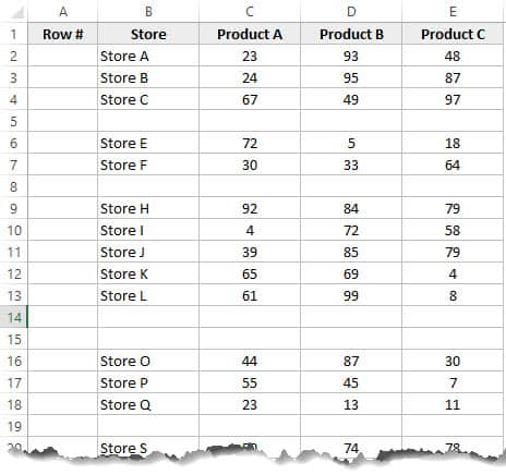
For example, if you have a dataset of different stores in a state, you may want to number the rows and so we have a unique number for each store.
Excel provides multiple ways to enter sequential numbers (also called serial numbers). In this tutorial we will look at 4 such ways:
- Using the Fill handle feature
- Using the ROW function
- Using the SEQUENCE function
- Converting the dataset into a table
Let us take a look at each of these methods one by one to enter serial numbers in Excel.
Using the Fill Handle Feature to Enter Sequential Numbers in Excel
Excel’s Fill Handle feature is smart enough to identify patterns in your data and project the pattern to the rest of the cells in a column.
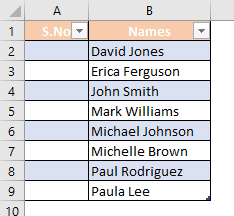
Say you have the following dataset and you want to enter a sequence of numbers starting from 1 (in the second row) all the way to the last row.
Here’s how you can quickly fill in Column A with a number sequence using the fill handle:
- Enter the number 1 in cell A2.
- Enter the number 2 in cell A3.
- Select both cells (A2 and A3). You should see a fill handle (small green square) at the bottom right corner of your selection.
- Drag the fill handle down to the last row of your dataset (or simply double click the fill handle).
You should automatically get a whole sequence of consecutive numbers, one for each row.
Using the ROW Function to Enter Sequential Numbers in Excel
The above method works great if you simply need to add a sequence of identifiers for each row of your data.
However, your sequencing order will change as soon as you sort the data, or even if you insert/delete a row.
If you need to ensure that the sequencing of the numbers remains the same irrespective of any operations performed on your dataset, then a better option would be to use the ROW function.
The ROW function’s only task is to return the ROW number of the current row.
So if you type the =ROW() in cell A3 or B3 or any cell in row 3, you will get the value 3.
Since we want to start sequencing from the second row onwards (in our example). We can enter the following formula in cell A2:
=ROW()-1
The ROW() function in cell A2 returns the value 2, since it is in the second row.
However, subtracting 1 from the value returned ensures you get one value less for every row number. This means the value in A4 will be 3, and so on.
If, instead of the second row, you needed to start sequencing from the 5th row (say), then your formula would be:
=ROW()-4
Copy the formula down to the rest of the cells in column A using the fill handle.
You will now be left with a sequence of consecutive numbers, one for each row.
Note that numbering is not going to get messed up even if you sort your dataset or insert/delete rows (in case you insert a new row, just copy and paste the same formula for that new row).
In fact, when you insert a new blank row, the sequencing automatically adjusts itself to ensure that the new row gets its appropriate sequence number.
Converting the Dataset into an Excel Table
The above two methods work quite well, but you still need to re-sequence your serial numbers whenever you insert a new row.
If you don’t want to be bothered by this additional hassle, you could simply convert your dataset into a table!
Excel tables are a great tool when working with tabular data as they group the data into a single object, allowing for many additional benefits.
One of the many benefits is that the table automatically inserts formulae or updates them whenever you insert or delete a row in it.
Moreover, even if you add new rows to the end of the table, it automatically expands to include the new rows as part of the table.
This means less hassle for you in updating formulae, and once your table is set up, you never have to bother about updating your serial number column again.
To convert your dataset into an Excel table, follow the steps shown below:
- Select all cells of the dataset.
- Navigate to Insert->Table. Alternatively, you could simply press the shortcut CTRL+T from your keyboard.
- This opens the Create Table dialog box. Make sure the range specified under ‘Where is the data for your table’ is correct.
- If your selection included headers, then check the box next to ‘My table has headers’.
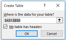
- Click OK.
Your selected range of cells should now get converted to an Excel table. You can tell by the change in the formatting of the table:
- Filter arrows appear next to each column header
- The dataset is enclosed in a distinguishable box
- The dataset is styled differently from the rest of the sheet. Rows of the table are styled in alternating colors.
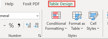
- When you click on any cell in the dataset, the Design (or Table Design) tab appears in the main menu.
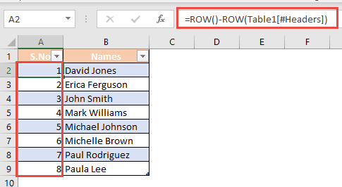
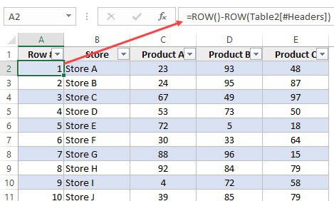
Once your table is ready, you can go ahead and enter the following formula in the first row of your table (cell A2):
=ROW()-ROW(Table1[#Headers])
The above formula simply takes the current row number and subtracts from it the row number of the header row of the current table.
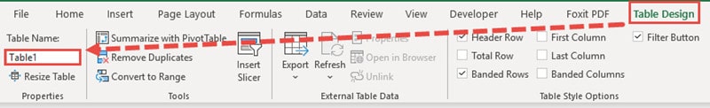
Here, we used Table1 as the name of the Excel table. You can replace this name with the name of your table.
Note: You will find the table name in the Design (or Table Design) tab, in an input box under the label ‘Table Name:’ (when you click on any cell of the table) :
When you press the return key, you should find column A containing a sequence of numbers starting from 1 in cell A2.
This method works irrespective of where your table is located.
Using the SEQUENCE Function to Enter Sequential Numbers in Excel (Only Available in Office 365 and Excel 2021)
Perhaps the easiest way to generate an array of sequential numbers is by using the SEQUENCE function.
The SEQUENCE function is a newly added Excel function. In fact, it is only available in newer versions, like Office 365 and Excel 2021.
This function basically generates sequential numbers in the form of a dynamic array. The syntax for this function is as follows:
SEQUENCE(rows, columns, start, step)
Here,
- rows is the number of rows that you want returned in the array
- columns is the number of columns that you want returned in the array .
- start is the number that you want the sequence to start from. This parameter is optional and by default this value is 1.
- step is the step value by which you want each number of the sequence to increase/decrease. This parameter is optional and by default, this value is 1.
Since we only want a single column of sequential numbers, it is enough to just specify the first parameter in the function. We do not need to add the optional parameters.
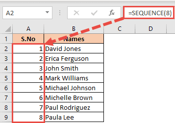
In our example, we want to generate a sequence of 8 consecutive numbers. So we can type the following function in cell A2:
=SEQUENCE(8)
You get an array of 8 sequential numbers displayed in column A as shown:
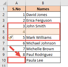
If you insert a new row into your data, you will notice that the sequence in column A remains put.
However you only have an 8-item array, so your sequence will only last till number 8, even though we now have a new row in our dataset.
Does that mean we have to update the parameter in the SEQUENCE function every time there is an addition or deletion of a row?
Absolutely not.
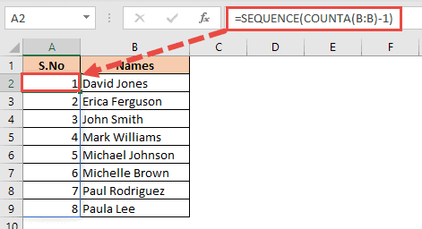
We can use the COUNTA function to keep track of the last row containing data. The following formula should work better:
=SEQUENCE(COUNTA(B:B)-1)
Try removing a row from the dataset.
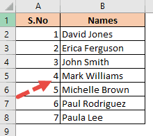
You will notice that the sequence now gets adjusted to display values till number 7 only.
When you introduce a new row into the dataset and enter some data into it, notice the sequencing gets adjusted to accommodate the new row.
The sequencing also expands as you add newer rows to the end of the dataset.
Note: If your column B contained numeric values (not text), then use the COUNT function instead of COUNTA.
Explanation of the Formula
The COUNTA function simply counts the number of non-null values in a given column.
In our example, the formula: =COUNTA(B:B) will return the value 9, since there are 9 cells in column B (including the header).
But we want to start sequencing from the second row onwards (excluding the header), so we need to subtract 1 from the value returned by the COUNTA function.
Once you get this number, you can then pass it to a SEQUENCE function to get a dynamic array of numbers that change according to the number of rows in column B:
=SEQUENCE(COUNTA(B:B)-1)
When you use this function, you get a sequence of numbers from 1 to 8 (in our case), starting from cell A2.
In this tutorial, we showed you four ways to enter sequential numbers in Excel.
The first method is quite volatile and the sequencing gets easily messed up whenever you alter rows of the dataset.
The second method does away with this issue, but you will still need to re-sequence every time you add, insert or delete a row.
The third method is much more robust, but it involves completely reformatting your dataset into an Excel table.
The fourth method is quite robust as it lets you keep the original formatting of your dataset.
However, the function used in this method (the SEQUENCE function) is only available in newer Excel versions like Office 365 and Excel 2021.
Each method differs in its application and usefulness. You can apply the method that most suits your data.
Other articles you may also like:
- How to Print Row Numbers in Excel
- How to Remove Duplicate Rows based on one Column in Excel?
- How to Flip Data in Excel (Columns, Rows, Tables)?
- How to Make Positive Numbers Negative in Excel
- How to Add a Total Row in Excel Table
- How to Press Enter in Excel and Stay in the Same Cell?
Watch Video – 7 Quick and Easy Ways to Number Rows in Excel
When working with Excel, there are some small tasks that need to be done quite often. Knowing the ‘right way’ can save you a great deal of time.
One such simple (yet often needed) task is to number the rows of a dataset in Excel (also called the serial numbers in a dataset).
Now if you’re thinking that one of the ways is to simply enter these serial number manually, well – you’re right!
But that’s not the best way to do it.
Imagine having hundreds or thousands of rows for which you need to enter the row number. It would be tedious – and completely unnecessary.
There are many ways to number rows in Excel, and in this tutorial, I am going to share some of the ways that I recommend and often use.
Of course, there would be more, and I will be waiting – with a coffee – in the comments area to hear from you about it.
How to Number Rows in Excel
The best way to number the rows in Excel would depend on the kind of data set that you have.
For example, you may have a continuous data set that starts from row 1, or a dataset that start from a different row. Or, you might have a dataset that has a few blank rows in it, and you only want to number the rows that are filled.
You can choose any one of the methods that work based on your dataset.
1] Using Fill Handle
Fill handle identifies a pattern from a few filled cells and can easily be used to quickly fill the entire column.
Suppose you have a dataset as shown below:

Here are the steps to quickly number the rows using the fill handle:
Note that Fill Handle automatically identifies the pattern and fill the remaining cells with that pattern. In this case, the pattern was that the numbers were getting incrementing by 1.
In case you have a blank row in the dataset, fill handle would only work till the last contiguous non-blank row.
Also, note that in case you don’t have data in the adjacent column, double-clicking the fill handle would not work. You can, however, place the cursor on the fill handle, hold the right mouse key and drag down. It will fill the cells covered by the cursor dragging.
2] Using Fill Series
While Fill Handle is a quick way to number rows in Excel, Fill Series gives you a lot more control over how the numbers are entered.
Suppose you have a dataset as shown below:
Here are the steps to use Fill Series to number rows in Excel:
This will instantly number the rows from 1 to 26.
Using ‘Fill Series’ can be useful when you’re starting by entering the row numbers. Unlike Fill Handle, it doesn’t require the adjacent columns to be filled already.
Even if you have nothing on the worksheet, Fill Series would still work.
Note: In case you have blank rows in the middle of the dataset, Fill Series would still fill the number for that row.
3] Using the ROW Function
You can also use Excel functions to number the rows in Excel.
In the Fill Handle and Fill Series methods above, the serial number inserted is a static value. This means that if you move the row (or cut and paste it somewhere else in the dataset), the row numbering will not change accordingly.
This shortcoming can be tackled using formulas in Excel.
You can use the ROW function to get the row numbering in Excel.
To get the row numbering using the ROW function, enter the following formula in the first cell and copy for all the other cells:
=ROW()-1
The ROW() function gives the row number of the current row. So I have subtracted 1 from it as I started from the second row onwards. If your data starts from the 5th row, you need to use the formula =ROW()-4.
The best part about using the ROW function is that it will not screw up the numberings if you delete a row in your dataset.
Since the ROW function is not referencing any cell, it will automatically (or should I say AutoMagically) adjust to give you the correct row number. Something as shown below:

Note that as soon as I delete a row, the row numbers automatically update.
Again, this would not take into account any blank records in the dataset. In case you have blank rows, it will still show the row number.
You can use the following formula to hide the row number for blank rows, but it would still not adjust the row numbers (such that the next row number is assigned to the next filled row).
IF(ISBLANK(B2),"",ROW()-1)
4] Using the COUNTA Function
If you want to number rows in a way that only the ones that are filled get a serial number, then this method is the way to go.
It uses the COUNTA function that counts the number of cells in a range that are not empty.
Suppose you have a dataset as shown below:
Note that there are blank rows in the above-shown dataset.
Here is the formula that will number the rows without numbering the blank rows.
=IF(ISBLANK(B2),"",COUNTA($B$2:B2))
The IF function checks whether the adjacent cell in column B is empty or not. If it’s empty, it returns a blank, but if it’s not, it returns the count of all the filled cells till that cell.
5] Using SUBTOTAL For Filtered Data
Sometimes, you may have a huge dataset, where you want to filter the data and then copy and paste the filtered data into a separate sheet.
If you use any of the methods shown above so far, you will notice that the row numbers remain the same. This means that when you copy the filtered data, you will have to update the row numbering.
In such cases, the SUBTOTAL function can automatically update the row numbers. Even when you filter the data set, the row numbers will remain intact.
Let me show you exactly how it works with an example.
Suppose you have a dataset as shown below:

If I filter this data based on Product A sales, you will get something as shown below:

Note that the serial numbers in Column A are also filtered. So now, you only see the numbers for the rows that are visible.
While this is the expected behavior, in case you want to get a serial row numbering – so that you can simply copy and paste this data somewhere else – you can use the SUBTOTAL function.
Here is the SUBTOTAL function that will make sure that even the filtered data has continuous row numbering.
=SUBTOTAL(3,$B$2:B2)
The 3 in the SUBTOTAL function specifies using the COUNTA function. The second argument is the range on which COUNTA function is applied.
The benefit of the SUBTOTAL function is that it dynamically updates when you filter the data (as shown below):

Note that even when the data is filtered, the row numbering update and remains continuous.
6] Creating an Excel Table
Excel Table is a great tool that you must use when working with tabular data. It makes managing and using data a lot easier.
This is also my favorite method among all the techniques shown in this tutorial.
Let me first show you the right way to number the rows using an Excel Table:
Note that in the formula above, I have used Table2, as that is the name of my Excel table. You can replace Table2 with the name of the table you have.
There are some added benefits of using an Excel Table while numbering rows in Excel:
- Since Excel Table automatically inserts the formula in the entire column, it works when you insert a new row in the Table. This means that when you insert/delete rows in an Excel Table, the row numbering would automatically update (as shown below).

- If you add more rows to the data, Excel Table would automatically expand to include this data as a part of the table. And since the formulas automatically update in the calculated columns, it would insert the row number for the newly inserted row (as shown below).


7] Adding 1 to the Previous Row Number
This is a simple method that works.
The idea is to add 1 to the previous row number (the number in the cell above). This will make sure that subsequent rows get a number that is incremented by 1.
Suppose you have a dataset as shown below:
Here are the steps to enter row numbers using this method:
- In the cell in the first row, enter 1 manually. In this case, it’s in cell A2.
- In cell A3, enter the formula, =A2+1
- Copy and paste the formula for all the cells in the column.

The above steps would enter serial numbers in all the cells in the column. In case there are any blank rows, this would still insert the row number for it.
Also note that in case you insert a new row, the row number would not update. In case you delete a row, all the cells below the deleted row would show a reference error.
These are some quick ways you can use to insert serial numbers in tabular data in Excel.
In case you are using any other method, do share it with me in the comments section.
You May Also Like the Following Excel Tutorials:
- Delete Blank Rows in Excel (with and without VBA).
- How to Insert Multiple Rows in Excel (4 Methods).
- How to Split Multiple Lines in a Cell into a Separate Cells / Columns.
- 7 Amazing Things Excel Text to Columns Can Do For You.
- Highlight EVERY Other ROW in Excel.
- How to Compare Two Columns in Excel.
- Insert New Columns in Excel
Applying serial number in a filtered list is a thorny problem. If you hard code the serial number or use the autofill function, the number will be renumbered automatically. In that case, you will have to manually change the number again.
In this article, I will show you two ways to apply serial number after filter. The first way is to add a new column of serial number and the second way is to make the serial number renumber automatically.
Sample
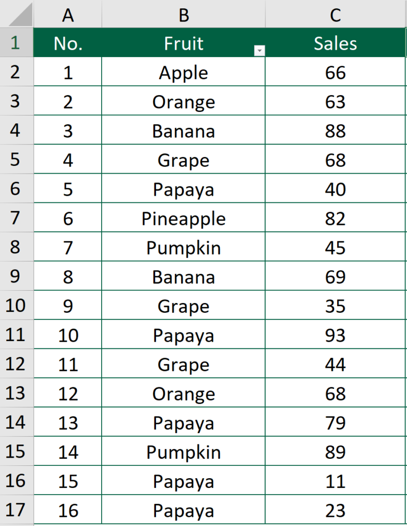
What we would like to do
To have number sequence when the filter is applied
You might also be interested in Edit The Same Cell In Multiple Excel Sheets
Apply serial number after filter in Excel by adding a column
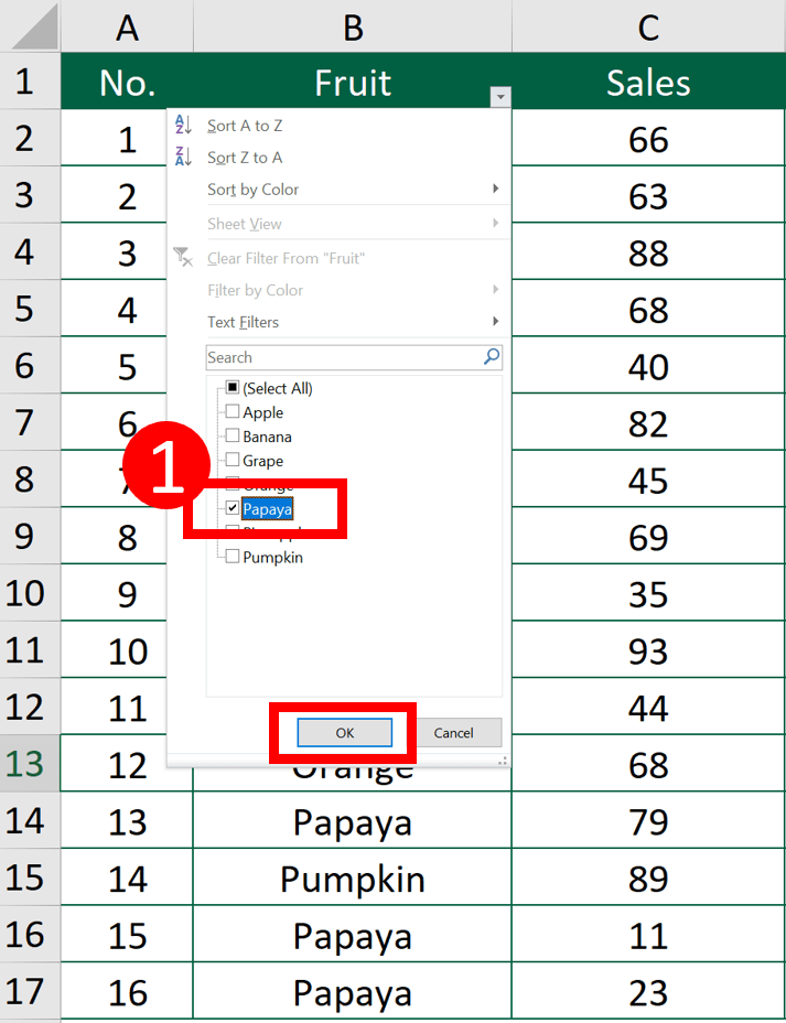
Step 1: Apply the filter as usual
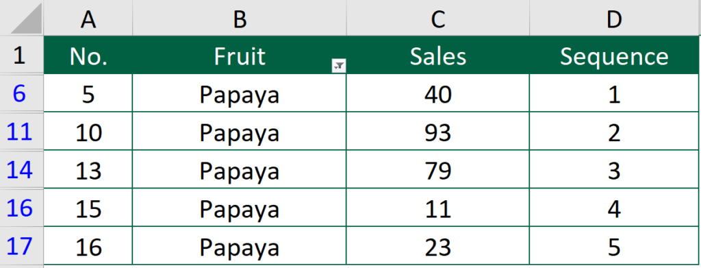
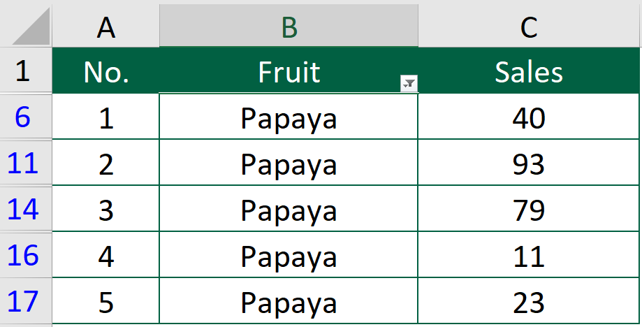
In this case, I only kept the “Papaya” in the column.
Step 2: Add a new column
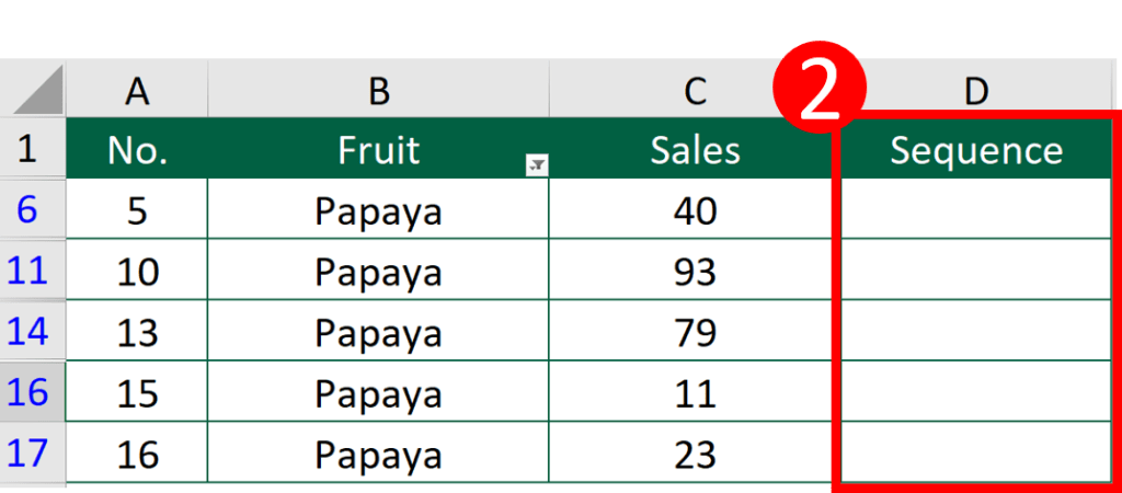
Step 3: Enter this formula in Cell D6
=COUNTA($D$1:D5)
In this example, I will enter the formula in cell D6. You will have to adjust the formula a bit when you use it.
If the condition is like this:
- you are entering the serial number in column B,
- the first cell of the sequence is in row 11,
Then the formula will be like this
=COUNTA($B$1:B10)
Step 4: Copy the formula down
You might also be interested in How to split Excel sheets into separate workbooks
Apply serial number that will renumber automatically
The beauty of this method is that you don’t have to repeat the above process when the filter is changed. After you applied the formula below, the serial number will renumber automatically.
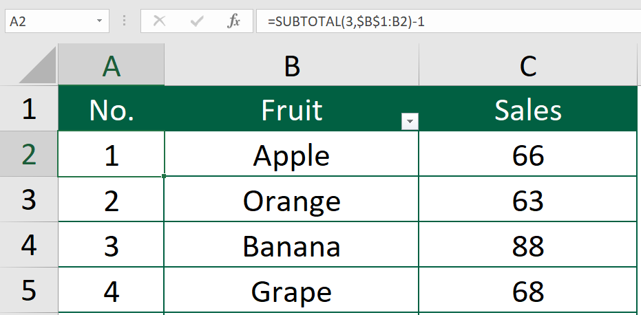
Step 1: Enter this formula in cell A2
=SUBTOTAL(3,$B$1:B2)-1
If the serial number is in column G, then you should change the above formula to =SUBTOTAL(3,$H$1:H2)-1.
Step 2: Copy the formula down
For example, the formula in cell A3 should be =SUBTOTAL(3,$B$1:B3)-1
What will happen when filter is applied
Let’s say I would like to display “Papaya” only.
The number in column A will renumber automatically.
Hungry for more useful Excel tips like this? Subscribe to our newsletter to make sure you won’t miss out on any of our posts and get exclusive Excel tips!
Microsoft’s office software Excel is a powerful tool to perform day-to-day activities with, like simple arithmetic, sorting, filtering, arranging and summarising data in various formats. Excel has a huge collection of formulas which can be used independently or in conjunction with each other to achieve desired results. This article will show you how to create serial numbers.
How to create serial numbers in Excel?
Logical formulas can be combined with text or numeric functions to segregate data in any desired way, such as excluding rows that do not have serial numbers. The same formula can be applied to multiple cells by simply dragging it to them or by using paste-special with formulas and number formats.
Assumptions:
- 1. You want series to appear in Column A
- 2. If a row has a data, then column B of that row would have data
- 3. Row 1 is a header
Write in Cell A2
=IF($B2="","",COUNTA($B$2:$B2))
Drag this formula down
any more excel questions? check out our forum!