
Split text into different columns with functions
Excel for Microsoft 365 Excel for Microsoft 365 for Mac Excel for the web Excel 2021 Excel 2021 for Mac Excel 2019 Excel 2019 for Mac Excel 2016 Excel 2016 for Mac Excel 2013 Excel Web App Excel 2010 Excel 2007 Excel for Mac 2011 More…Less
You can use the LEFT, MID, RIGHT, SEARCH, and LEN text functions to manipulate strings of text in your data. For example, you can distribute the first, middle, and last names from a single cell into three separate columns.
The key to distributing name components with text functions is the position of each character within a text string. The positions of the spaces within the text string are also important because they indicate the beginning or end of name components in a string.
For example, in a cell that contains only a first and last name, the last name begins after the first instance of a space. Some names in your list may contain a middle name, in which case, the last name begins after the second instance of a space.
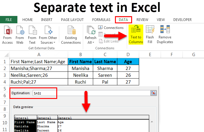
This article shows you how to extract various components from a variety of name formats using these handy functions. You can also split text into different columns with the Convert Text to Columns Wizard
|
Example name |
Description |
First name |
Middle name |
Last name |
Suffix |
|
|
1 |
Jeff Smith |
No middle name |
Jeff |
Smith |
||
|
2 |
Eric S. Kurjan |
One middle initial |
Eric |
S. |
Kurjan |
|
|
3 |
Janaina B. G. Bueno |
Two middle initials |
Janaina |
B. G. |
Bueno |
|
|
4 |
Kahn, Wendy Beth |
Last name first, with comma |
Wendy |
Beth |
Kahn |
|
|
5 |
Mary Kay D. Andersen |
Two-part first name |
Mary Kay |
D. |
Andersen |
|
|
6 |
Paula Barreto de Mattos |
Three-part last name |
Paula |
Barreto de Mattos |
||
|
7 |
James van Eaton |
Two-part last name |
James |
van Eaton |
||
|
8 |
Bacon Jr., Dan K. |
Last name and suffix first, with comma |
Dan |
K. |
Bacon |
Jr. |
|
9 |
Gary Altman III |
With suffix |
Gary |
Altman |
III |
|
|
10 |
Mr. Ryan Ihrig |
With prefix |
Ryan |
Ihrig |
||
|
11 |
Julie Taft-Rider |
Hyphenated last name |
Julie |
Taft-Rider |
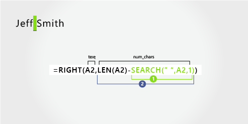
Note: In the graphics in the following examples, the highlight in the full name shows the character that the matching SEARCH formula is looking for.
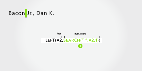
This example separates two components: first name and last name. A single space separates the two names.
Copy the cells in the table and paste into an Excel worksheet at cell A1. The formula you see on the left will be displayed for reference, while Excel will automatically convert the formula on the right into the appropriate result.
Hint Before you paste the data into the worksheet, set the column widths of columns A and B to 250.
|
Example name |
Description |
|
Jeff Smith |
No middle name |
|
Formula |
Result (first name) |
|
‘=LEFT(A2, SEARCH(» «,A2,1)) |
=LEFT(A2, SEARCH(» «,A2,1)) |
|
Formula |
Result (last name) |
|
‘=RIGHT(A2,LEN(A2)-SEARCH(» «,A2,1)) |
=RIGHT(A2,LEN(A2)-SEARCH(» «,A2,1)) |
-
First name
The first name starts with the first character in the string (J) and ends at the fifth character (the space). The formula returns five characters in cell A2, starting from the left.

Use the SEARCH function to find the value for num_chars:
Search for the numeric position of the space in A2, starting from the left.
-
Last name
The last name starts at the space, five characters from the right, and ends at the last character on the right (h). The formula extracts five characters in A2, starting from the right.
Use the SEARCH and LEN functions to find the value for num_chars:
Search for the numeric position of the space in A2, starting from the left. (5)
-
Count the total length of the text string, and then subtract the number of characters to the left of the first space, as found in step 1.

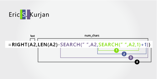
This example uses a first name, middle initial, and last name. A space separates each name component.
Copy the cells in the table and paste into an Excel worksheet at cell A1. The formula you see on the left will be displayed for reference, while Excel will automatically convert the formula on the right into the appropriate result.
Hint Before you paste the data into the worksheet, set the column widths of columns A and B to 250.
|
Example name |
Description |
|
Eric S. Kurjan |
One middle initial |
|
Formula |
Result (first name) |
|
‘=LEFT(A2, SEARCH(» «,A2,1)) |
=LEFT(A2, SEARCH(» «,A2,1)) |
|
Formula |
Result (middle initial) |
|
‘=MID(A2,SEARCH(» «,A2,1)+1,SEARCH(» «,A2,SEARCH(» «,A2,1)+1)-SEARCH(» «,A2,1)) |
=MID(A2,SEARCH(» «,A2,1)+1,SEARCH(» «,A2,SEARCH(» «,A2,1)+1)-SEARCH(» «,A2,1)) |
|
Formula |
Live Result (last name) |
|
‘=RIGHT(A2,LEN(A2)-SEARCH(» «,A2,SEARCH(» «,A2,1)+1)) |
=RIGHT(A2,LEN(A2)-SEARCH(» «,A2,SEARCH(» «,A2,1)+1)) |
-
First name
The first name starts with the first character from the left (E) and ends at the fifth character (the first space). The formula extracts the first five characters in A2, starting from the left.
Use the SEARCH function to find the value for num_chars:
Search for the numeric position of the space in A2, starting from the left. (5)
-
Middle name
The middle name starts at the sixth character position (S), and ends at the eighth position (the second space). This formula involves nesting SEARCH functions to find the second instance of a space.
The formula extracts three characters, starting from the sixth position.
Use the SEARCH function to find the value for start_num:
Search for the numeric position of the first space in A2, starting from the first character from the left. (5).
-
Add 1 to get the position of the character after the first space (S). This numeric position is the starting position of the middle name. (5 + 1 = 6)
Use nested SEARCH functions to find the value for num_chars:
Search for the numeric position of the first space in A2, starting from the first character from the left. (5)
-
Add 1 to get the position of the character after the first space (S). The result is the character number at which you want to start searching for the second instance of space. (5 + 1 = 6)
-
Search for the second instance of space in A2, starting from the sixth position (S) found in step 4. This character number is the ending position of the middle name. (8)
-
Search for the numeric position of space in A2, starting from the first character from the left. (5)
-
Take the character number of the second space found in step 5 and subtract the character number of the first space found in step 6. The result is the number of characters MID extracts from the text string starting at the sixth position found in step 2. (8 – 5 = 3)
-
Last name
The last name starts six characters from the right (K) and ends at the first character from the right (n). This formula involves nesting SEARCH functions to find the second and third instances of a space (which are at the fifth and eighth positions from the left).
The formula extracts six characters in A2, starting from the right.
-
Use the LEN and nested SEARCH functions to find the value for num_chars:
Search for the numeric position of space in A2, starting from the first character from the left. (5)
-
Add 1 to get the position of the character after the first space (S). The result is the character number at which you want to start searching for the second instance of space. (5 + 1 = 6)
-
Search for the second instance of space in A2, starting from the sixth position (S) found in step 2. This character number is the ending position of the middle name. (8)
-
Count the total length of the text string in A2, and then subtract the number of characters from the left up to the second instance of space found in step 3. The result is the number of characters to be extracted from the right of the full name. (14 – 8 = 6).


Here’s an example of how to extract two middle initials. The first and third instances of space separate the name components.
Copy the cells in the table and paste into an Excel worksheet at cell A1. The formula you see on the left will be displayed for reference, while Excel will automatically convert the formula on the right into the appropriate result.
Hint Before you paste the data into the worksheet, set the column widths of columns A and B to 250.
|
Example name |
Description |
|
Janaina B. G. Bueno |
Two middle initials |
|
Formula |
Result (first name) |
|
‘=LEFT(A2, SEARCH(» «,A2,1)) |
=LEFT(A2, SEARCH(» «,A2,1)) |
|
Formula |
Result (middle initials) |
|
‘=MID(A2,SEARCH(» «,A2,1)+1,SEARCH(» «,A2,SEARCH(» «,A2,SEARCH(» «,A2,1)+1)+1)-SEARCH(» «,A2,1)) |
=MID(A2,SEARCH(» «,A2,1)+1,SEARCH(» «,A2,SEARCH(» «,A2,SEARCH(» «,A2,1)+1)+1)-SEARCH(» «,A2,1)) |
|
Formula |
Live Result (last name) |
|
‘=RIGHT(A2,LEN(A2)-SEARCH(» «,A2,SEARCH(» «,A2,SEARCH(» «,A2,1)+1)+1)) |
=RIGHT(A2,LEN(A2)-SEARCH(» «,A2,SEARCH(» «,A2,SEARCH(» «,A2,1)+1)+1)) |
-
First name
The first name starts with the first character from the left (J) and ends at the eighth character (the first space). The formula extracts the first eight characters in A2, starting from the left.
Use the SEARCH function to find the value for num_chars:
Search for the numeric position of the first space in A2, starting from the left. (8)
-
Middle name
The middle name starts at the ninth position (B), and ends at the fourteenth position (the third space). This formula involves nesting SEARCH to find the first, second, and third instances of space in the eighth, eleventh, and fourteenth positions.
The formula extracts five characters, starting from the ninth position.
Use the SEARCH function to find the value for start_num:
Search for the numeric position of the first space in A2, starting from the first character from the left. (8)
-
Add 1 to get the position of the character after the first space (B). This numeric position is the starting position of the middle name. (8 + 1 = 9)
Use nested SEARCH functions to find the value for num_chars:
Search for the numeric position of the first space in A2, starting from the first character from the left. (8)
-
Add 1 to get the position of the character after the first space (B). The result is the character number at which you want to start searching for the second instance of space. (8 + 1 = 9)
-
Search for the second space in A2, starting from the ninth position (B) found in step 4. (11).
-
Add 1 to get the position of the character after the second space (G). This character number is the starting position at which you want to start searching for the third space. (11 + 1 = 12)
-
Search for the third space in A2, starting at the twelfth position found in step 6. (14)
-
Search for the numeric position of the first space in A2. (8)
-
Take the character number of the third space found in step 7 and subtract the character number of the first space found in step 6. The result is the number of characters MID extracts from the text string starting at the ninth position found in step 2.
-
Last name
The last name starts five characters from the right (B) and ends at the first character from the right (o). This formula involves nesting SEARCH to find the first, second, and third instances of space.
The formula extracts five characters in A2, starting from the right of the full name.
Use nested SEARCH and the LEN functions to find the value for the num_chars:
Search for the numeric position of the first space in A2, starting from the first character from the left. (8)
-
Add 1 to get the position of the character after the first space (B). The result is the character number at which you want to start searching for the second instance of space. (8 + 1 = 9)
-
Search for the second space in A2, starting from the ninth position (B) found in step 2. (11)
-
Add 1 to get the position of the character after the second space (G). This character number is the starting position at which you want to start searching for the third instance of space. (11 + 1 = 12)
-
Search for the third space in A2, starting at the twelfth position (G) found in step 6. (14)
-
Count the total length of the text string in A2, and then subtract the number of characters from the left up to the third space found in step 5. The result is the number of characters to be extracted from the right of the full name. (19 — 14 = 5)


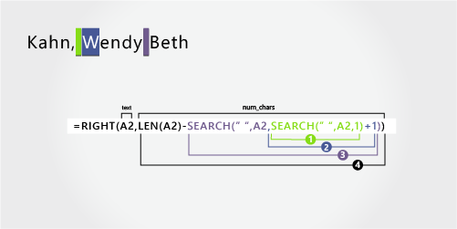
In this example, the last name comes before the first, and the middle name appears at the end. The comma marks the end of the last name, and a space separates each name component.
Copy the cells in the table and paste into an Excel worksheet at cell A1. The formula you see on the left will be displayed for reference, while Excel will automatically convert the formula on the right into the appropriate result.
Hint Before you paste the data into the worksheet, set the column widths of columns A and B to 250.
|
Example name |
Description |
|
Kahn, Wendy Beth |
Last name first, with comma |
|
Formula |
Result (first name) |
|
‘=MID(A2,SEARCH(» «,A2,1)+1,SEARCH(» «,A2,SEARCH(» «,A2,1)+1)-SEARCH(» «,A2,1)) |
=MID(A2,SEARCH(» «,A2,1)+1,SEARCH(» «,A2,SEARCH(» «,A2,1)+1)-SEARCH(» «,A2,1)) |
|
Formula |
Result (middle name) |
|
‘=RIGHT(A2,LEN(A2)-SEARCH(» «,A2,SEARCH(» «,A2,1)+1)) |
=RIGHT(A2,LEN(A2)-SEARCH(» «,A2,SEARCH(» «,A2,1)+1)) |
|
Formula |
Live Result (last name) |
|
‘=LEFT(A2, SEARCH(» «,A2,1)-2) |
=LEFT(A2, SEARCH(» «,A2,1)-2) |
-
First name
The first name starts with the seventh character from the left (W) and ends at the twelfth character (the second space). Because the first name occurs at the middle of the full name, you need to use the MID function to extract the first name.
The formula extracts six characters, starting from the seventh position.
Use the SEARCH function to find the value for start_num:
Search for the numeric position of the first space in A2, starting from the first character from the left. (6)
-
Add 1 to get the position of the character after the first space (W). This numeric position is the starting position of the first name. (6 + 1 = 7)
Use nested SEARCH functions to find the value for num_chars:
Search for the numeric position of the first space in A2, starting from the first character from the left. (6)
-
Add 1 to get the position of the character after the first space (W). The result is the character number at which you want to start searching for the second space. (6 + 1 = 7)
Search for the second space in A2, starting from the seventh position (W) found in step 4. (12)
-
Search for the numeric position of the first space in A2, starting from the first character from the left. (6)
-
Take the character number of the second space found in step 5 and subtract the character number of the first space found in step 6. The result is the number of characters MID extracts from the text string starting at the seventh position found in step 2. (12 — 6 = 6)
-
Middle name
The middle name starts four characters from the right (B), and ends at the first character from the right (h). This formula involves nesting SEARCH to find the first and second instances of space in the sixth and twelfth positions from the left.
The formula extracts four characters, starting from the right.
Use nested SEARCH and the LEN functions to find the value for start_num:
Search for the numeric position of the first space in A2, starting from the first character from the left. (6)
-
Add 1 to get the position of the character after the first space (W). The result is the character number at which you want to start searching for the second space. (6 + 1 = 7)
-
Search for the second instance of space in A2 starting from the seventh position (W) found in step 2. (12)
-
Count the total length of the text string in A2, and then subtract the number of characters from the left up to the second space found in step 3. The result is the number of characters to be extracted from the right of the full name. (16 — 12 = 4)
-
Last name
The last name starts with the first character from the left (K) and ends at the fourth character (n). The formula extracts four characters, starting from the left.
Use the SEARCH function to find the value for num_chars:
Search for the numeric position of the first space in A2, starting from the first character from the left. (6)
-
Subtract 2 to get the numeric position of the ending character of the last name (n). The result is the number of characters you want LEFT to extract. (6 — 2 =4)


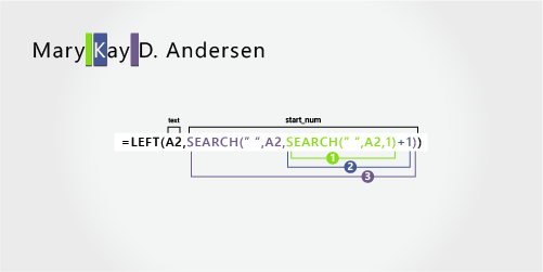
This example uses a two-part first name, Mary Kay. The second and third spaces separate each name component.
Copy the cells in the table and paste into an Excel worksheet at cell A1. The formula you see on the left will be displayed for reference, while Excel will automatically convert the formula on the right into the appropriate result.
Hint Before you paste the data into the worksheet, set the column widths of columns A and B to 250.
|
Example name |
Description |
|
Mary Kay D. Andersen |
Two-part first name |
|
Formula |
Result (first name) |
|
LEFT(A2, SEARCH(» «,A2,SEARCH(» «,A2,1)+1)) |
=LEFT(A2, SEARCH(» «,A2,SEARCH(» «,A2,1)+1)) |
|
Formula |
Result (middle initial) |
|
‘=MID(A2,SEARCH(» «,A2,SEARCH(» «,A2,1)+1)+1,SEARCH(» «,A2,SEARCH(» «,A2,SEARCH(» «,A2,1)+1)+1)-(SEARCH(» «,A2,SEARCH(» «,A2,1)+1)+1)) |
=MID(A2,SEARCH(» «,A2,SEARCH(» «,A2,1)+1)+1,SEARCH(» «,A2,SEARCH(» «,A2,SEARCH(» «,A2,1)+1)+1)-(SEARCH(» «,A2,SEARCH(» «,A2,1)+1)+1)) |
|
Formula |
Live Result (last name) |
|
‘=RIGHT(A2,LEN(A2)-SEARCH(» «,A2,SEARCH(» «,A2,SEARCH(» «,A2,1)+1)+1)) |
=RIGHT(A2,LEN(A2)-SEARCH(» «,A2,SEARCH(» «,A2,SEARCH(» «,A2,1)+1)+1)) |
-
First name
The first name starts with the first character from the left and ends at the ninth character (the second space). This formula involves nesting SEARCH to find the second instance of space from the left.
The formula extracts nine characters, starting from the left.
Use nested SEARCH functions to find the value for num_chars:
Search for the numeric position of the first space in A2, starting from the first character from the left. (5)
-
Add 1 to get the position of the character after the first space (K). The result is the character number at which you want to start searching for the second instance of space. (5 + 1 = 6)
-
Search for the second instance of space in A2, starting from the sixth position (K) found in step 2. The result is the number of characters LEFT extracts from the text string. (9)
-
Middle name
The middle name starts at the tenth position (D), and ends at the twelfth position (the third space). This formula involves nesting SEARCH to find the first, second, and third instances of space.
The formula extracts two characters from the middle, starting from the tenth position.
Use nested SEARCH functions to find the value for start_num:
Search for the numeric position of the first space in A2, starting from the first character from the left. (5)
-
Add 1 to get the character after the first space (K). The result is the character number at which you want to start searching for the second space. (5 + 1 = 6)
-
Search for the position of the second instance of space in A2, starting from the sixth position (K) found in step 2. The result is the number of characters LEFT extracts from the left. (9)
-
Add 1 to get the character after the second space (D). The result is the starting position of the middle name. (9 + 1 = 10)
Use nested SEARCH functions to find the value for num_chars:
Search for the numeric position of the character after the second space (D). The result is the character number at which you want to start searching for the third space. (10)
-
Search for the numeric position of the third space in A2, starting from the left. The result is the ending position of the middle name. (12)
-
Search for the numeric position of the character after the second space (D). The result is the beginning position of the middle name. (10)
-
Take the character number of the third space, found in step 6, and subtract the character number of “D”, found in step 7. The result is the number of characters MID extracts from the text string starting at the tenth position found in step 4. (12 — 10 = 2)
-
Last name
The last name starts eight characters from the right. This formula involves nesting SEARCH to find the first, second, and third instances of space in the fifth, ninth, and twelfth positions.
The formula extracts eight characters from the right.
Use nested SEARCH and the LEN functions to find the value for num_chars:
Search for the numeric position of the first space in A2, starting from the left. (5)
-
Add 1 to get the character after the first space (K). The result is the character number at which you want to start searching for the space. (5 + 1 = 6)
-
Search for the second space in A2, starting from the sixth position (K) found in step 2. (9)
-
Add 1 to get the position of the character after the second space (D). The result is the starting position of the middle name. (9 + 1 = 10)
-
Search for the numeric position of the third space in A2, starting from the left. The result is the ending position of the middle name. (12)
-
Count the total length of the text string in A2, and then subtract the number of characters from the left up to the third space found in step 5. The result is the number of characters to be extracted from the right of the full name. (20 — 12 =


This example uses a three-part last name: Barreto de Mattos. The first space marks the end of the first name and the beginning of the last name.
Copy the cells in the table and paste into an Excel worksheet at cell A1. The formula you see on the left will be displayed for reference, while Excel will automatically convert the formula on the right into the appropriate result.
Hint Before you paste the data into the worksheet, set the column widths of columns A and B to 250.
|
Example name |
Description |
|
Paula Barreto de Mattos |
Three-part last name |
|
Formula |
Result (first name) |
|
‘=LEFT(A2, SEARCH(» «,A2,1)) |
=LEFT(A2, SEARCH(» «,A2,1)) |
|
Formula |
Result (last name) |
|
RIGHT(A2,LEN(A2)-SEARCH(» «,A2,1)) |
=RIGHT(A2,LEN(A2)-SEARCH(» «,A2,1)) |
-
First name
The first name starts with the first character from the left (P) and ends at the sixth character (the first space). The formula extracts six characters from the left.
Use the Search function to find the value for num_chars:
Search for the numeric position of the first space in A2, starting from the left. (6)
-
Last name
The last name starts seventeen characters from the right (B) and ends with first character from the right (s). The formula extracts seventeen characters from the right.
Use the LEN and SEARCH functions to find the value for num_chars:
Search for the numeric position of the first space in A2, starting from the left. (6)
-
Count the total length of the text string in A2, and then subtract the number of characters from the left up to the first space, found in step 1. The result is the number of characters to be extracted from the right of the full name. (23 — 6 = 17)


This example uses a two-part last name: van Eaton. The first space marks the end of the first name and the beginning of the last name.
Copy the cells in the table and paste into an Excel worksheet at cell A1. The formula you see on the left will be displayed for reference, while Excel will automatically convert the formula on the right into the appropriate result.
Hint Before you paste the data into the worksheet, set the column widths of columns A and B to 250.
|
Example name |
Description |
|
James van Eaton |
Two-part last name |
|
Formula |
Result (first name) |
|
‘=LEFT(A2, SEARCH(» «,A2,1)) |
=LEFT(A2, SEARCH(» «,A2,1)) |
|
Formula |
Result (last name) |
|
‘=RIGHT(A2,LEN(A2)-SEARCH(» «,A2,1)) |
=RIGHT(A2,LEN(A2)-SEARCH(» «,A2,1)) |
-
First name
The first name starts with the first character from the left (J) and ends at the eighth character (the first space). The formula extracts six characters from the left.
Use the SEARCH function to find the value for num_chars:
Search for the numeric position of the first space in A2, starting from the left. (6)
-
Last name
The last name starts with the ninth character from the right (v) and ends at the first character from the right (n). The formula extracts nine characters from the right of the full name.
Use the LEN and SEARCH functions to find the value for num_chars:
Search for the numeric position of the first space in A2, starting from the left. (6)
-
Count the total length of the text string in A2, and then subtract the number of characters from the left up to the first space, found in step 1. The result is the number of characters to be extracted from the right of the full name. (15 — 6 = 9)


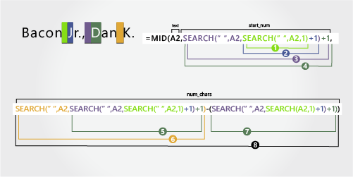
In this example, the last name comes first, followed by the suffix. The comma separates the last name and suffix from the first name and middle initial.
Copy the cells in the table and paste into an Excel worksheet at cell A1. The formula you see on the left will be displayed for reference, while Excel will automatically convert the formula on the right into the appropriate result.
Hint Before you paste the data into the worksheet, set the column widths of columns A and B to 250.
|
Example name |
Description |
|
Bacon Jr., Dan K. |
Last name and suffix first, with comma |
|
Formula |
Result (first name) |
|
‘=MID(A2,SEARCH(» «,A2,SEARCH(» «,A2,1)+1)+1,SEARCH(» «,A2,SEARCH(» «,A2,SEARCH(» «,A2,1)+1)+1)-SEARCH(» «,A2,SEARCH(» «,A2,1)+1)) |
=MID(A2,SEARCH(» «,A2,SEARCH(» «,A2,1)+1)+1,SEARCH(» «,A2,SEARCH(» «,A2,SEARCH(» «,A2,1)+1)+1)-SEARCH(» «,A2,SEARCH(» «,A2,1)+1)) |
|
Formula |
Result (middle initial) |
|
‘=RIGHT(A2,LEN(A2)-SEARCH(» «,A2,SEARCH(» «,A2,SEARCH(» «,A2,1)+1)+1)) |
=RIGHT(A2,LEN(A2)-SEARCH(» «,A2,SEARCH(» «,A2,SEARCH(» «,A2,1)+1)+1)) |
|
Formula |
Result (last name) |
|
‘=LEFT(A2, SEARCH(» «,A2,1)) |
=LEFT(A2, SEARCH(» «,A2,1)) |
|
Formula |
Result (suffix) |
|
‘=MID(A2,SEARCH(» «, A2,1)+1,(SEARCH(» «,A2,SEARCH(» «,A2,1)+1)-2)-SEARCH(» «,A2,1)) |
=MID(A2,SEARCH(» «, A2,1)+1,(SEARCH(» «,A2,SEARCH(» «,A2,1)+1)-2)-SEARCH(» «,A2,1)) |
-
First name
The first name starts with the twelfth character (D) and ends with the fifteenth character (the third space). The formula extracts three characters, starting from the twelfth position.
Use nested SEARCH functions to find the value for start_num:
Search for the numeric position of the first space in A2, starting from the left. (6)
-
Add 1 to get the character after the first space (J). The result is the character number at which you want to start searching for the second space. (6 + 1 = 7)
-
Search for the second space in A2, starting from the seventh position (J), found in step 2. (11)
-
Add 1 to get the character after the second space (D). The result is the starting position of the first name. (11 + 1 = 12)
Use nested SEARCH functions to find the value for num_chars:
Search for the numeric position of the character after the second space (D). The result is the character number at which you want to start searching for the third space. (12)
-
Search for the numeric position of the third space in A2, starting from the left. The result is the ending position of the first name. (15)
-
Search for the numeric position of the character after the second space (D). The result is the beginning position of the first name. (12)
-
Take the character number of the third space, found in step 6, and subtract the character number of “D”, found in step 7. The result is the number of characters MID extracts from the text string starting at the twelfth position, found in step 4. (15 — 12 = 3)
-
Middle name
The middle name starts with the second character from the right (K). The formula extracts two characters from the right.
Search for the numeric position of the first space in A2, starting from the left. (6)
-
Add 1 to get the character after the first space (J). The result is the character number at which you want to start searching for the second space. (6 + 1 = 7)
-
Search for the second space in A2, starting from the seventh position (J), found in step 2. (11)
-
Add 1 to get the character after the second space (D). The result is the starting position of the first name. (11 + 1 = 12)
-
Search for the numeric position of the third space in A2, starting from the left. The result is the ending position of the middle name. (15)
-
Count the total length of the text string in A2, and then subtract the number of characters from the left up to the third space, found in step 5. The result is the number of characters to be extracted from the right of the full name. (17 — 15 = 2)
-
Last name
The last name starts at the first character from the left (B) and ends at sixth character (the first space). Therefore, the formula extracts six characters from the left.
Use the SEARCH function to find the value for num_chars:
Search for the numeric position of the first space in A2, starting from the left. (6)
-
Suffix
The suffix starts at the seventh character from the left (J), and ends at ninth character from the left (.). The formula extracts three characters, starting from the seventh character.
Use the SEARCH function to find the value for start_num:
Search for the numeric position of the first space in A2, starting from the left. (6)
-
Add 1 to get the character after the first space (J). The result is the starting position of the suffix. (6 + 1 = 7)
Use nested SEARCH functions to find the value for num_chars:
Search for the numeric position of the first space in A2, starting from the left. (6)
-
Add 1 to get the numeric position of the character after the first space (J). The result is the character number at which you want to start searching for the second space. (7)
-
Search for the numeric position of the second space in A2, starting from the seventh character found in step 4. (11)
-
Subtract 1 from the character number of the second space found in step 4 to get the character number of “,”. The result is the ending position of the suffix. (11 — 1 = 10)
-
Search for the numeric position of the first space. (6)
-
After finding the first space, add 1 to find the next character (J), also found in steps 3 and 4. (7)
-
Take the character number of “,” found in step 6, and subtract the character number of “J”, found in steps 3 and 4. The result is the number of characters MID extracts from the text string starting at the seventh position, found in step 2. (10 — 7 = 3)


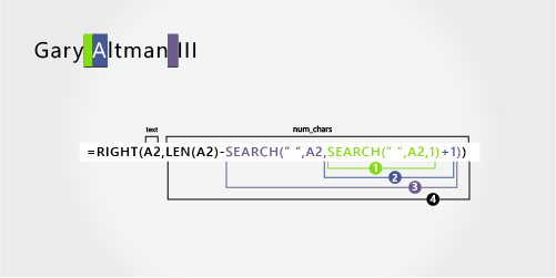
In this example, the first name is at the beginning of the string and the suffix is at the end, so you can use formulas similar to Example 2: Use the LEFT function to extract the first name, the MID function to extract the last name, and the RIGHT function to extract the suffix.
Copy the cells in the table and paste into an Excel worksheet at cell A1. The formula you see on the left will be displayed for reference, while Excel will automatically convert the formula on the right into the appropriate result.
Hint Before you paste the data into the worksheet, set the column widths of columns A and B to 250.
|
Example name |
Description |
|
Gary Altman III |
First and last name with suffix |
|
Formula |
Result (first name) |
|
‘=LEFT(A2, SEARCH(» «,A2,1)) |
=LEFT(A2, SEARCH(» «,A2,1)) |
|
Formula |
Result (last name) |
|
‘=MID(A2,SEARCH(» «,A2,1)+1,SEARCH(» «,A2,SEARCH(» «,A2,1)+1)-(SEARCH(» «,A2,1)+1)) |
=MID(A2,SEARCH(» «,A2,1)+1,SEARCH(» «,A2,SEARCH(» «,A2,1)+1)-(SEARCH(» «,A2,1)+1)) |
|
Formula |
Result (suffix) |
|
‘=RIGHT(A2,LEN(A2)-SEARCH(» «,A2,SEARCH(» «,A2,1)+1)) |
=RIGHT(A2,LEN(A2)-SEARCH(» «,A2,SEARCH(» «,A2,1)+1)) |
-
First name
The first name starts at the first character from the left (G) and ends at the fifth character (the first space). Therefore, the formula extracts five characters from the left of the full name.
Search for the numeric position of the first space in A2, starting from the left. (5)
-
Last name
The last name starts at the sixth character from the left (A) and ends at the eleventh character (the second space). This formula involves nesting SEARCH to find the positions of the spaces.
The formula extracts six characters from the middle, starting from the sixth character.
Use the SEARCH function to find the value for start_num:
Search for the numeric position of the first space in A2, starting from the left. (5)
-
Add 1 to get the position of the character after the first space (A). The result is the starting position of the last name. (5 + 1 = 6)
Use nested SEARCH functions to find the value for num_chars:
Search for the numeric position of the first space in A2, starting from the left. (5)
-
Add 1 to get the position of the character after the first space (A). The result is the character number at which you want to start searching for the second space. (5 + 1 = 6)
-
Search for the numeric position of the second space in A2, starting from the sixth character found in step 4. This character number is the ending position of the last name. (12)
-
Search for the numeric position of the first space. (5)
-
Add 1 to find the numeric position of the character after the first space (A), also found in steps 3 and 4. (6)
-
Take the character number of the second space, found in step 5, and then subtract the character number of “A”, found in steps 6 and 7. The result is the number of characters MID extracts from the text string, starting at the sixth position, found in step 2. (12 — 6 = 6)
-
Suffix
The suffix starts three characters from the right. This formula involves nesting SEARCH to find the positions of the spaces.
Use nested SEARCH and the LEN functions to find the value for num_chars:
Search for the numeric position of the first space in A2, starting from the left. (5)
-
Add 1 to get the character after the first space (A). The result is the character number at which you want to start searching for the second space. (5 + 1 = 6)
-
Search for the second space in A2, starting from the sixth position (A), found in step 2. (12)
-
Count the total length of the text string in A2, and then subtract the number of characters from the left up to the second space, found in step 3. The result is the number of characters to be extracted from the right of the full name. (15 — 12 = 3)


In this example, the full name is preceded by a prefix, and you use formulas similar to Example 2: the MID function to extract the first name, the RIGHT function to extract the last name.
Copy the cells in the table and paste into an Excel worksheet at cell A1. The formula you see on the left will be displayed for reference, while Excel will automatically convert the formula on the right into the appropriate result.
Hint Before you paste the data into the worksheet, set the column widths of columns A and B to 250.
|
Example name |
Description |
|
Mr. Ryan Ihrig |
With prefix |
|
Formula |
Result (first name) |
|
‘=MID(A2,SEARCH(» «,A2,1)+1,SEARCH(» «,A2,SEARCH(» «,A2,1)+1)-(SEARCH(» «,A2,1)+1)) |
=MID(A2,SEARCH(» «,A2,1)+1,SEARCH(» «,A2,SEARCH(» «,A2,1)+1)-(SEARCH(» «,A2,1)+1)) |
|
Formula |
Result (last name) |
|
‘=RIGHT(A2,LEN(A2)-SEARCH(» «,A2,SEARCH(» «,A2,1)+1)) |
=RIGHT(A2,LEN(A2)-SEARCH(» «,A2,SEARCH(» «,A2,1)+1)) |
-
First name
The first name starts at the fifth character from the left (R) and ends at the ninth character (the second space). The formula nests SEARCH to find the positions of the spaces. It extracts four characters, starting from the fifth position.
Use the SEARCH function to find the value for the start_num:
Search for the numeric position of the first space in A2, starting from the left. (4)
-
Add 1 to get the position of the character after the first space (R). The result is the starting position of the first name. (4 + 1 = 5)
Use nested SEARCH function to find the value for num_chars:
Search for the numeric position of the first space in A2, starting from the left. (4)
-
Add 1 to get the position of the character after the first space (R). The result is the character number at which you want to start searching for the second space. (4 + 1 = 5)
-
Search for the numeric position of the second space in A2, starting from the fifth character, found in steps 3 and 4. This character number is the ending position of the first name. (9)
-
Search for the first space. (4)
-
Add 1 to find the numeric position of the character after the first space (R), also found in steps 3 and 4. (5)
-
Take the character number of the second space, found in step 5, and then subtract the character number of “R”, found in steps 6 and 7. The result is the number of characters MID extracts from the text string, starting at the fifth position found in step 2. (9 — 5 = 4)
-
Last name
The last name starts five characters from the right. This formula involves nesting SEARCH to find the positions of the spaces.
Use nested SEARCH and the LEN functions to find the value for num_chars:
Search for the numeric position of the first space in A2, starting from the left. (4)
-
Add 1 to get the position of the character after the first space (R). The result is the character number at which you want to start searching for the second space. (4 + 1 = 5)
-
Search for the second space in A2, starting from the fifth position (R), found in step 2. (9)
-
Count the total length of the text string in A2, and then subtract the number of characters from the left up to the second space, found in step 3. The result is the number of characters to be extracted from the right of the full name. (14 — 9 = 5)


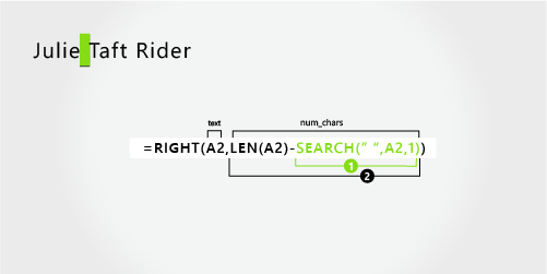
This example uses a hyphenated last name. A space separates each name component.
Copy the cells in the table and paste into an Excel worksheet at cell A1. The formula you see on the left will be displayed for reference, while Excel will automatically convert the formula on the right into the appropriate result.
Hint Before you paste the data into the worksheet, set the column widths of columns A and B to 250.
|
Example name |
Description |
|
Julie Taft-Rider |
Hyphenated last name |
|
Formula |
Result (first name) |
|
‘=LEFT(A2, SEARCH(» «,A2,1)) |
=LEFT(A2, SEARCH(» «,A2,1)) |
|
Formula |
Result (last name) |
|
‘=RIGHT(A2,LEN(A2)-SEARCH(» «,A2,1)) |
=RIGHT(A2,LEN(A2)-SEARCH(» «,A2,1)) |
-
First name
The first name starts at the first character from the left and ends at the sixth position (the first space). The formula extracts six characters from the left.
Use the SEARCH function to find the value of num_chars:
Search for the numeric position of the first space in A2, starting from the left. (6)
-
Last name
The entire last name starts ten characters from the right (T) and ends at the first character from the right (r).
Use the LEN and SEARCH functions to find the value for num_chars:
Search for the numeric position of the space in A2, starting from the first character from the left. (6)
-
Count the total length of the text string to be extracted, and then subtract the number of characters from the left up to the first space, found in step 1. (16 — 6 = 10)

Need more help?
Want more options?
Explore subscription benefits, browse training courses, learn how to secure your device, and more.
Communities help you ask and answer questions, give feedback, and hear from experts with rich knowledge.
One scenario is where you need to join multiple strings of text into a single text string. The flip of that is splitting a single text string into multiple text strings. If the data at hand was copied from somewhere or created by someone who completely missed the point of Excel columns, you will find that you need to split a block of text to categorize it.
Splitting the text largely depends on the delimiter in the text string. A delimiter is a character or symbol that marks the beginning or end of a character string. Examples of a delimiter are a space character, hyphen, period, comma.
 1")
Our example case for this guide involves splitting book details into book title, author, and genre. The delimiter we’ve used is a comma:
 2")
This tutorial will teach you how to split text in Excel with the Text to Columns and Flash Fill features, formulas, and VBA. The formulas method includes splitting text by a specific character. That’s the menu today.
Let’s get splitting!
Using Text to Columns
This feature lives up to its name. Text to Columns splits a column of text into multiple columns with specified controls. Text to Columns can split text with delimiters and since our data contains only a comma as the delimiter, using the feature becomes very easy. See the following steps to split text using Text to Columns:
- Select the data you want to split.
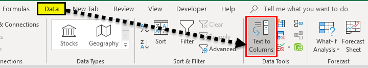
- Go to the Data tab and select the Text to Columns icon from the Data Tools
 3")
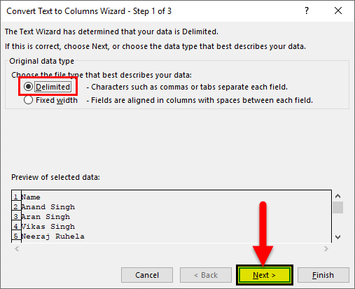
- Select the Delimited radio button and then click on the Next
 4")
- In the Delimiters section, select the Comma
- Then select the Next button.
 5")
- Now you need to choose where you want the split text. Click on the Destination field, then select the destination cell on the worksheet in the background where you want the split text to start.
- Select the Finish button to close the Text to Columns
 6")
Using the comma delimiter to separate the text string, Text to Columns has split the text from our example case into three columns:
 7")
Luckily, our data doesn’t contain a book with commas in the book name. If we had the book Cows, Pigs, Wars and Witches by Marvin Harris in the dataset, the text would be split into 5 columns instead of 3 like the rest. If the delimiter in your data is appearing in the text string for more than delimiting, you’ll have better luck splitting text with other methods. Now unto another observation.
Using TRIM Function to Trim Extra Spaces
Let’s cast a closer look at the output of Text to Columns. Notice how the last two columns carry one leading space? You can see that the values in columns D and E are not a hundred percent aligned to the left:
 8")
The last two columns carry a leading space because Text to Columns only takes the delimiter as a mark from where to split the text. The space character after the comma is carried with the next unit of text and that has our data with a leading space.
A quick fix for this is to use the TRIM function to clear up extra spaces. Here is the formula we have used to remove leading spaces from columns D and E:
=TRIM(C4)
The TRIM function removes all spaces from a text string other than a single space character between two words. Any leading, trailing, or extra spaces will be removed from the cell’s value. We have simply used the formula with a reference of the cell containing the leading space.
And that cleaned up the leading spaces for us. Data – good to go!
 9")
Using Formula To Separate Text in Excel
We can make use to Excel functions to construct formulas that can help us in splitting a text string into multiple.
Split String with Delimiter
Using a formula can also split a single text string into multiple strings but it will require a combo of functions. Let’s have a little briefing on the functions that make part of this formula we will use for splitting text.
The SUBSTITUTE function replaces old text in a text string with new text.
The REPT function repeats text a given number of times.
The LEN function returns the number of characters in a text string.
The MID function returns a given number of characters from the middle of a text string with a specified starting position.
The TRIM function removes all spaces, other than single spaces between words, from a text string.
Now let’s see how these functions combined can be used to split text with a single formula:
=TRIM(MID(SUBSTITUTE($B5,",",REPT(" ",LEN($B5))),(C$4-1)*LEN($B5)+1,LEN($B5)))
In our example, the first cell we are using this formula on is cell B5. The number of characters in B5 as counted by the LEN function is 49. The REPT function repeats spaces (denoted by “ “ in the formula) in B5 for the number of characters supplied by the LEN function i.e. 49.
The SUBSTITUTE function replaces the commas “,” in B5 with 49 space characters supplied by the REPT function. Since there are two commas in B5, one after the book name and one after the author, 49 spaces will be entered after the book name and 49 spaces after the author, creating a decent gap between the text we want to split.
Now let’s see the calculations for the MID function. The first bit is (C$4-1). In row 4, we added serial numbering for each of the columns for our categories. The row has been locked in the formula with a $ sign so the row doesn’t change as the formula is copied down. But we have left the column free so that the serial number changes for the respective columns used in the formula.
In the formula, 1 is subtracted from C4 (1-1=0) and the result is multiplied by the number of characters in B5 i.e. LEN($B5) and then 1 is added to the expression. The calculation for the starting position in the MID function, i.e. (C$4-1)*LEN($B5)+1, becomes (1-1)*49+1 which equals 1.
The MID function returns the text from the middle of B5, the starting position is 1 (that means the text to be returned is to start from the first character) and the number of characters to be returned is LEN($B5) i.e 49 characters. Since we have added 49 spaces in place of each of the commas, that gives us plenty of area to safely return just one chunk of text along with some extra spaces. The result up until the MID function is A Song of Ice and Fire with lots of trailing spaces.
The extra spaces are no problem. The TRIM function cleans any extra spaces leaving the single spaces between words and so we finally have the book name returned as A Song of Ice and Fire.
 10")
Now for the next column and hence the next category, the calculation for the starting position in the MID function will change like so (D$4-1)*LEN($B5)+1. The expression comes down to (2-1)*49+1 which equals 50. If the MID function is to return characters starting from the 50th character, with all the extra spaces added by the REPT function, what the MID function will return will be along this pattern: spaces author spaces.
The leading and trailing spaces will be trimmed by the TRIM function and the result will be George RR Martin.
 11")
The “+1” in the starting position argument of the MID function has no relevance for the subsequent columns, only for the first. That is because, without the “+1” in the first column’s calculation, it would be 0*49 which will end up in a #VALUE! error.
The formula copied along column E gives us the genre from the combined text in column B and that completes our set.
Split String at Specific Character
If there is only a single delimiter that is a specific character, such a lengthy formula as above will not be required to split the text. Let’s say, like our case example below, we are to split product code and product type which is joined by a hyphen.
Now this would be easier if the product code had a fixed number of characters; we would only have to use the LEFT function to return a certain number of characters. But what’s the fun in that?
We are going to let the FIND function do a bit of search work for us and find the hyphen in the text so the LEFT function and RIGHT function can return the surrounding text. This is the formula with the LEFT function for returning the first extract:
=LEFT(B3,FIND("-",B3)-1)
The FIND function searches B3 for the position of the hyphen “-“ in the text string, which is 6. The LEFT function then returns the characters starting from the left of the text and the number of characters to return is 6-1. “-1” at the end ensures that the characters returned do not include the hyphen itself. Here are the results of this formula for returning the first segment of split text:
 12")
Now for the second segment of text, the RIGHT function comes into play with this formula:
=RIGHT(B3,LEN(B3)-FIND("-",B3))
The FIND function is again used to find the location of the hyphen in B3 which we know is the 6th character. The LEN function returns the number of characters in B3 as 23. The RIGHT function extracts 23-6 characters from B3 and returns the product type “Bluetooth Speaker”. This is how it has worked for our example:
 13")
Using Flash Fill
The Flash Fill feature in Excel automatically fills in values based on a couple of manually provided examples. The ease of Flash Fill is that you need not remember any formulas, use any wizards, or fiddle with any settings. If your data is consistent, Flash Fill will be the quickest to pick up on what you are trying to get done. Let’s see the steps for using Flash Fill to split text and how it works for our example case:
- Type the first text as an example for Flash Fill to pick up the pattern and press the Enter
 14")
- From the Home tab’s Editing group, click on the Fill icon and select Flash Fill from the menu.
- Alternatively, use the shortcut keys Ctrl + E.
 15")
- Picking up on the provided example, Flash Fill will split the text and fill the column according to the same pattern:
 16")
- Repeat the same steps for each column to be Flash-Filled.
 17")
Flash Fill will save the trouble of having to trim leading and trailing spaces but as mentioned, if there are any anomalies or inconsistencies in the data (e.g a space before and after the comma), Flash Fill won’t be a reliable method of splitting text and due to the bulk of the data, the problem may go ignored. If you doubt the data to have inconsistencies, use the other methods for splitting the text.
Using VBA Function
The final method we will be discussing today for splitting text will be a VBA function. In order to automate tasks in MS Office applications, macros can be created and used with VBA. Our task is to split text in Excel and below are the steps for doing this using VBA:
- If you have the Developer tab added to the toolbar Ribbon, click on the Developer tab and then select the Visual Basic icon in the Code group to launch the Visual Basic
- You can also use the Alt + F11 keys.
 18")
- The Visual Basic editor will have opened:
 19")
- Open the Insert tab and select Module from the list. A Module window will open.
 20")
- In the Module window, copy-paste the following code to create a macro titled SplitText:
Sub SplitText()
Dim MyArray() As String, Count As Long, i As Variant
For n = 4 To 16
 MyArray = Split(Cells(n, 2), ",")
 Count = 3
 For Each i In MyArray
 Cells(n, Count) = i
 Count = Count + 1
 Next i
Next n
End Sub
Edit the following parts of the code as per your data:
- ‘For n = 4 To 16’ – 4 and 16 represent the first and last rows of the dataset.
- ‘MyArray = Split(Cells(n, 2), «,»)’ – The comma enclosed with double quotes is the delimiter.
- ‘Count = 3’ – 3 is the column number of the first column that the resulting data will be returned in.
 21")
- To run the code, press the F5
The data will be split as per the supplied values:
- Clean up the leading spaces in columns D and E using the TRIM function:
Now let’s split the active guide from its conclusion. Today you learned a few ways on how to split text in Excel. If you find yourself splitting hairs on your ability to split text next time, pocket this one and be ready to give it a go! We’ll be back with more Excel-ness to fill your pockets. Make some space!
Separating Text in Excel
The texts in Excel can appear in different ways. For example, maybe there is a text joined by some symbol, or it is like a first name and the last name.
At some point in our life, we will want those texts separated. The problem statement is explained above that we will come towards some data where we need to separate those texts from one another. But how do we separate those texts from one another? There is one very basic way to do it: copy the desired text in each selected individual cell. Else, we can use some pre-given Excel tools to perform.
Table of contents
- Separating Text in Excel
- How to Separate Text in Excel?
- Example #1 – Delimiter Method to Separate Text
- Example #2 – Using the Fixed Width Method to Separate Text
- Example #3 – Using Formulas for Separating Text
- Things to Remember in Separating Text in Excel (text to column & formula)
- Recommended Articles
- How to Separate Text in Excel?
How to Separate Text in Excel?
There are two methods to separate Texts in Excel:
- Using “Text to Columns in ExcelText to columns in excel is used to separate text in different columns based on some delimited or fixed width. This is done either by using a delimiter such as a comma, space or hyphen, or using fixed defined width to separate a text in the adjacent columns.read more“: It further has its own two bifurcations:
- Delimited: This feature splits the text, which is joined by characters, commas, tabs, spaces, semicolons, or any other character such as a hyphen (-).
- Fixed Width: This feature splits the text, which is joined with spaces with a certain width.
- Using Excel Formulas: We can use formulas like the Len in excelThe Len function returns the length of a given string. It calculates the number of characters in a given string as input. It is a text function in Excel as well as an inbuilt function that can be accessed by typing =LEN( and entering a string as input.read more to calculate the length of the string and separate the values by knowing the position of the characters
Let us learn these methods using examples.
You can download this Separate Text Excel Template here – Separate Text Excel Template
Example #1 – Delimiter Method to Separate Text
First, where do we find this feature text to columns in Excel? It is under the “Data” tab in the “Data Tools” section.
Consider the following data,
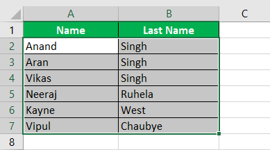
We want to separate the first and last names. Therefore, the last names’ content is in the B column.
Below are the steps of separating text in excel –
- First, we must select the column containing the data, A column.

- Under the “Data” tab in the “Data Tools” section, click on “Text to Columns.”

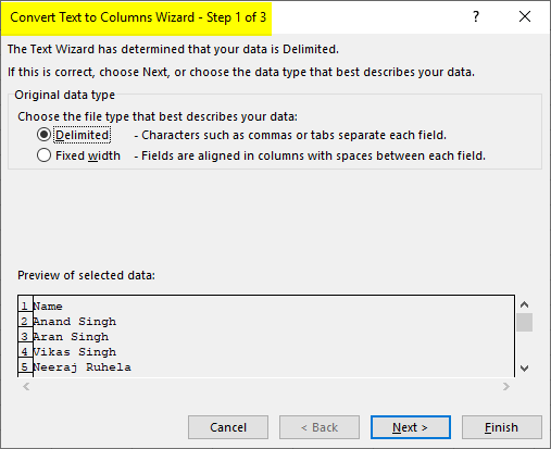
- A dialog box appears for text to columns wizard.

- As we will use the delimiter method first, select the “Delimited” option and click on “Next.” Another dialog box appears.
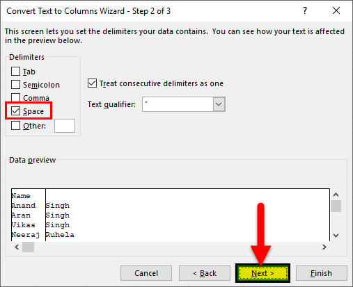
- Our texts are separated in Excel by spaces for the current data, so select the “Space” option as a “delimiter” ( By default, Excel selects a tab as a delimiter). Then, finally, click on “Next.”
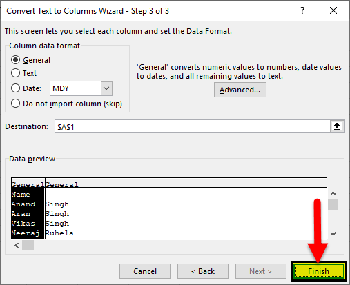
- Our “Data preview” shows that our texts are separated with first and last names. Click on “Finish” to see the result.
- We have successfully separated our Excel text by using the text-to-column delimiter method.

Example #2 – Using the Fixed Width Method to Separate Text
We already know where the option of text to the column is in Excel. It is in the “Data” tab under the “Data Tools” section.
Now we consider the following data,
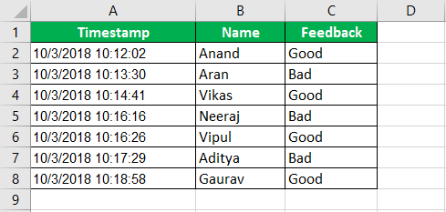
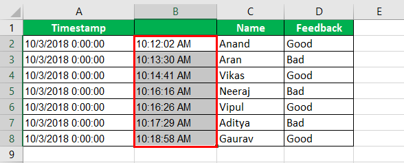
There is a survey company that is surveying for the feedback of a restaurant. The users give their feedback as “Good” or “Bad.” But every response is saved by a timestamp, which means with every response, time is recorded, specific data and time in hours and minutes.
We need to separate the date from the time in the data. Below is the data.
Step #1 – We need to separate the contents of column A, but there is data in column B, so we need to insert another column between columns A and B. Select column B and press the “CTRL + +” keys for that.
It adds another column between the columns and shifts the data from previous column B to column C.
Step #2 – Now, select the data in column A. Click on “Text to Columns” under the “Data” tab in the “Data Tools” section.
A dialog box appears for converting text to columns wizard.
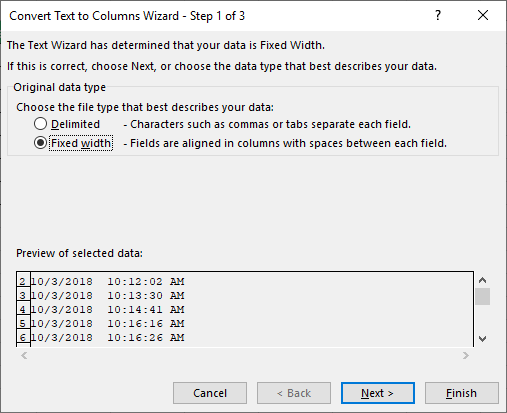
Step #3 – This time, we use a fixed width method. So ensure that the “Fixed width” method option is selected and click on “Next.” Another “Convert Text to Column Wizard” dialog box appears.
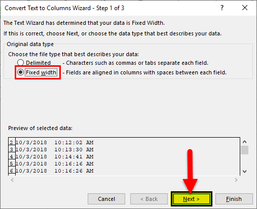
Step #4 – In the “Data preview,” we can see that the data is separated into three parts: date, time, and the meridian, AM, and PM.
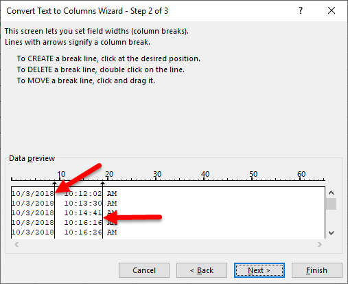
We need only date and time, so hover the mouse around the second line and double click on it, and it disappears.
Step #5 – Now, click “Next.” Another “Convert Text to Columns Wizard” dialog box appears. Then, you need to click on the “Finish” button.
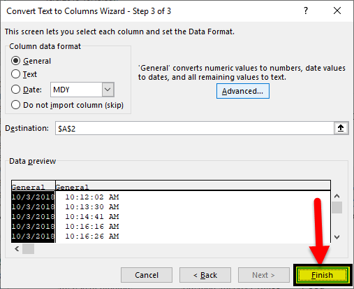
Now, the data is separated with date in one column and time in another.
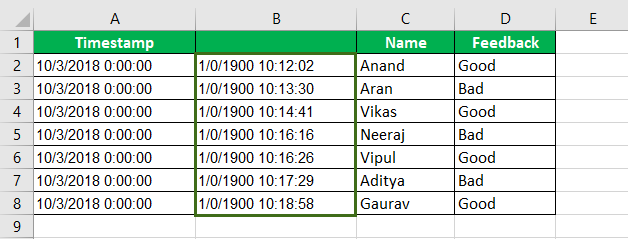
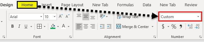
Step #6 – The data formatting in column B is incorrect, so we must rectify it. Select the contents on column B, and in the “Home” tab under the “Number” section, the default selection is “Custom.” We need to change it to “Time.”
Step #7 – We have successfully separated our Excel data using the “Text to Columns Fixed Width” method.
Example #3 – Using Formulas for Separating Text
We can also use Excel formulas to separate the text and numbers, which are joined together. Then, we can remove that data by using “Text to Columns.” However, we use formulas for complex situations.
Let us consider the following Data:
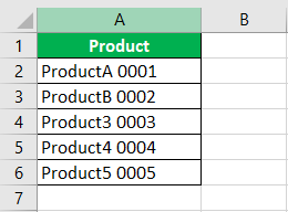
We have products in column A with their respective product codes. We need products in one column and product code in another. We want to use formulas to do this.
Step #1- To this, we must first count the number of digits and separate that number from the character.
Step #2- We need the “Product Name” in column B and “Product Code” in column C.
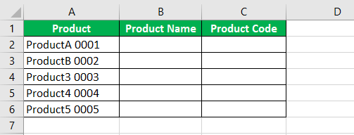
Step #3- First, we will separate the digits to separate the text in Excel from the data. In C2, write the following Excel formula to separate text.
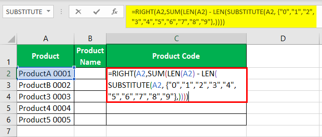
We use the right to function as we know the numbers are in the right.
Step #4- Now, in Cell B2, write the following Formula,
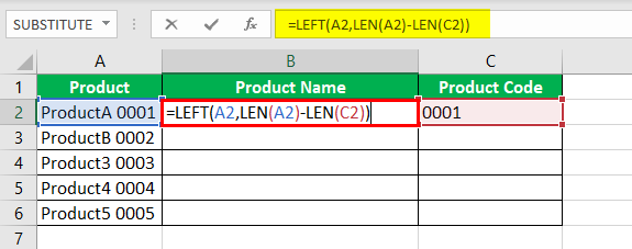
Step #5- Press the “Enter” key. Using the LEN function, we have successfully separated our data from “Product Name” and ” Product Code.”
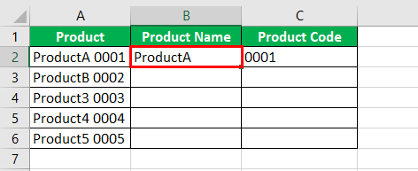
Step #6- Drag the formulas to cells B6 and C6, respectively.
Things to Remember in Separating Text in Excel (text to column & formula)
- If we use the “Text to Columns” method, always ensure that we have an additional column so that the data in any column does not get replaced.
- We must ensure the characters’ positioning if we separate texts in Excel using Excel formulas.
Recommended Articles
This article is a guide to Separate Text in Excel. Here, we discuss how to separate text in Excel using two methods: 1) Text to Columns (delimited and fixed width), and 2) Excel formulas with practical examples and a downloadable template. You may learn more about Excel from the following articles: –
- Date to Text in ExcelYou can convert Date to Text in Excel through the most commonly used method, i.e., the text function or by using: Text-to-Column option, Copy Paste Method and VBA.
read more - Convert Date to Text in ExcelTo convert a date to text in Excel, right-click on the date cell and select the format cells option. A new window will open. You can convert the date to text by selecting the desired format from a list of options.read more
- Numbers to Text in Excel with ExamplesYou may need to convert numbers to text in Excel for a variety of reasons. If you use Excel spreadsheets to store long and not-so-long numbers, or if you don’t want the numbers in the cells to be involved in calculating, or if you want to display leading zeros in numbers in cells, you’ll need to convert them to text at some point. It’s useful for displaying numbers in a more readable format or combining numbers with text or symbols. The methods listed below can be used to accomplish this.read more
- Top Excel Keyword Shortcuts
When data is imported into Excel it can be in many formats depending on the source application that has provided it.
For example, it could contain names and addresses of customers or employees, but this all ends up as a continuous text string in one column of the worksheet, instead of being separated out into individual columns e.g. name, street, city.
You can split the data by using a common delimiter character. A delimiter character is usually a comma, tab, space, or semi-colon. This character separates each chunk of data within the text string.
A big advantage of using a delimiter character is that it does not rely on fixed widths within the text. The delimiter indicates exactly where to split the text.
You may need to split the data because you may want to sort the data using a certain part of the address or to be able to filter on a particular component. If the data is used in a pivot table, you may need to have the name and address as different fields within it.
This article shows you eight ways to split the text into the component parts required by using a delimiter character to indicate the split points.
Sample Data
The above sample data will be used in all the following examples. Download the example file to get the sample data plus the various solutions for extracting data based on delimiters.
Excel Functions to Split Text
There are several Excel functions that can be used to split and manipulate text within a cell.
LEFT Function
The LEFT function returns the number of characters from the left of the text.
Syntax
= LEFT ( Text, [Number] )- Text – This is the text string that you wish to extract from. It can also be a valid cell reference within a workbook.
- Number [Optional] – This is the number of characters that you wish to extract from the text string. The value must be greater than or equal to zero. If the value is greater than the length of the text string, then all characters will be returned. If the value is omitted, then the value is assumed to be one.
RIGHT Function
The RIGHT function returns the number of characters from the right of the text.
Syntax
= RIGHT ( Text, [Number] )The parameters work in the same way as for the LEFT function described above.
FIND Function
The FIND function returns the position of specified text within a text string. This can be used for locating a delimiter character. Note that the search is case-sensitive.
Syntax
= FIND (SubText, Text, [Start])- SubText – This is a text string that you want to search for.
- Text – This is the text string which is to be searched.
- Start [Optional] – The starting position for the search.
LEN Function
The LEN function will give the length by number of characters of a text string.
Syntax
= LEN ( Text )- Text – This is the text string of which you want to determine the character count.
Extracting Data with the LEFT, RIGHT, FIND and LEN Functions
Using the first row (B3) of the sample data, these functions can be combined to split a text string into sections using a delimiter character.
= FIND ( ",", B3 )You use the FIND function to get the position of the first delimiter character. This will return the value 18.
= LEFT ( B3, FIND( ",", B3 ) - 1 )You can then use the LEFT function to extract the first component of the text string.
Note that FIND gets the position of the first delimiter, but you need to subtract 1 from it so as to not include the delimiter character.
This will return Tabbie O’Hallagan.
= RIGHT ( B3, LEN ( B3 ) - FIND ( ",", B3 ) )It is more complicated to get the next components of the text string. You need to remove the first component from the text by using the above formula.
This formula takes the length of the original text, finds the first delimiter position, which then calculates how many characters are left in the text string after that delimiter.
The RIGHT function then truncates off all the characters up to and including that first delimiter so that the text string gets shorter and shorter as each delimiter character is found.
This will return 056 Dennis Park, Greda, Croatia, 44273
You can now use FIND to locate the next delimiter and the LEFT function to extract the next component, using the same methodology as above.
Repeat for all delimiters, and this will split the text string into component parts.
FILTERXML Function as a Dynamic Array
If you’re using Excel for Microsoft 365, then you can use the FILTERXML function to split text with output as a dynamic array.
You can split a text string by turning it into an XML string by changing the delimiter characters to XML tags. This way you can use the FILTERXML function to extract data.
XML tags are user defined, but in this example, s will represent a sub-node and t will represent the main node.
= "<t><s>" & SUBSTITUTE ( B2, ",", "</s><s>" ) & "</s></t>"Use the above formula to insert the XML tags into your text string.
<t><s>Name</s><s>Street</s><s>City</s><s>Country</s><s>Post Code</s></t>This will return the above formula in the example.
Note that each of the nodes defined is followed by a closing node with a backslash. These XML tags define the start and finish of each section of the text, and effectively act in the same way as delimiters.
=TRANSPOSE(
    FILTERXML(
        "<t><s>" &
        SUBSTITUTE(
            B3,
            ",",
            "</s><s>"
        ) & "</s></t>",
        "//s"
    )
)
The above formula will insert the XML tags into the original string and then use these to split out the items into an array.
As seen above, the array will spill each item into a separate cell. Using the TRANSPOSE function causes the array to spill horizontally instead of vertically.
FILTERXML Function to Split Text
If your version of Excel doesn’t have dynamic arrays, then you can still use the FILTERXML function to extract individual items.
= FILTERXML (
    "<t><s>" &
    SUBSTITUTE (
        B3,
        ",",
        "</s><s>"
    ) & "</s></t>",
    "//s"
)
You can now break the string into sections using the above FILTERXML formula.
This will return the first section Tabbie O’Hallagan.
= FILTERXML (
    "<t><s>" &
    SUBSTITUTE (
        B3,
        ",",
        "</s><s>"
    ) & "</s></t>",
    "//s[2]"
)
To return the next section, use the above formula.
This will return the second section of the text string 056 Dennis Park.
You can use this same pattern to return any part of the sample text, just change the [2] found in the formula accordingly.
Flash Fill to Split Text
Flash Fill allows you to put in an example of how you want your data split.
You can check out this guide on using flash fill to clean your data for more details.
You then select the first cell of where you want your data to split and click on Flash Fill. Excel will populate the remaining rows from your example.
Using the sample data, enter Name into cell C2, then Tabbie O’Hallagan into cell C3.
Flash fill should automatically fill in the remaining data names from the sample data. If it doesn’t, you can select cell C4, and click on the Flash Fill icon in the Data Tools group of the Data tab of the Excel ribbon.
Similarly, you can add Street into cell D2, City into cell E2, Country into cell F2, and Post Code into cell G2.
Select the subsequent cells (D2 to G2) individually, and click on the Flash Fill icon. The rest of the text components will be populated into these columns.
Text to Columns Command to Split Text
This Excel functionality can be used to split text in a cell into sections based on a delimiter character.
- Select the entire sample data range (B2:B12).
- Click on the Data tab in the Excel ribbon.
- Click on the Text to Columns icon in the Data Tools group of the Excel ribbon and a wizard will appear to help you set up how the text will be split.
- Select Delimited on the option buttons.
- Press the Next button.
- Select Comma as the delimiter, and uncheck any other delimiters.
- Press the Next button.
- The Data Preview window will display how your data will be split. Choose a location to place the output.
- Click on Finish button.
Your data will now be displayed in columns on your worksheet.
Convert the Data into a CSV File
This will only work with commas as delimiters, since a CSV (comma separated value) file depends on commas to separate the values.
Open Notepad and copy and paste the sample data into it. You can open Notepad by typing Notepad into the search box at the left of the Windows task bar or locate it in the application list.
Once you have copied the data into Notepad, save it off by using File ➜ Save As from the menu. Enter a filename with a .csv suffix e.g. Split Data.csv.
You can then open this file in Excel. Select the csv file in the browser file type drop down and click OK. Your data will automatically appear with each component in separate columns.
VBA to Split Text
VBA is the programming language that sits behind Excel and allows you to write your own code to manipulate data, or to even create your own functions.
To access the Visual Basic Editor (VBE), you use Alt + F11.
Sub SplitText()

Dim MyArray() As String, Count As Long, i As Variant

For n = 2 To 12
	MyArray = Split(Cells(n, 2), ",")
	Count = 3
	For Each i In MyArray
		Cells(n, Count) = i
		Count = Count + 1
	Next i
Next n

End Sub
Click on Insert in the menu bar, and click on Module. A new pane will appear for the module. Paste in the above code.
This code creates a single dimensional array called MyArray. It then iterates through the sample data (rows 2 to 12) and uses the VBA Split function to populate MyArray.
The split function uses a comma delimiter, so that each section of the text becomes an element of the array.
A counter variable is set to 3 which represents column C, which will be the first column for the split data to be displayed.
The code then iterates through each element in the array and populates each cell with the element. Cell references are based on n for the row, and Count for the column.
The variable Count is incremented in each loop so that the data fills across the row, and then downwards.
Power Query to Split Text
Power Query in Excel allows a column to be manipulated into sections using a delimiter character.
Related posts:
- Introduction to power query
- Power query tips and tricks
- Introduction to power query M code
The first thing to do is to define your data source, which is the sample data that you entered into you Excel worksheet.
Click on the Data tab in the Excel ribbon, and then click on Get Data in the Get & Transform Data group of the ribbon.
Click on From File in the first drop down, and then click on From Workbook in the second drop down.
This will display a file browser. Locate your sample data file (the file that you have open) and click on OK.
A navigation pop-up will be displayed showing all the worksheets within your workbook. Click on the worksheet which has the sample data and this will show a preview of the data.
Expand the tree of data in the left-hand pane to show the preview of the existing data.
Click on Transform Data and this will display the Power Query Editor.
Make sure that the single column with the data in it is highlighted. Click on the Split Column icon in the Transform group of the ribbon. Click on By Delimiter in the drop down that appears.
This will display a pop-up window which allows you to select your delimiter. The default is a comma.
Click OK and the data will be transformed into separate columns.
Click on Close and Load in the Close group of the ribbon, and a new worksheet will be added to your workbook with a table of the data in the new format.
Power Pivot Calculated Column to Split Text
You can use Power Pivot to split the text by using calculated columns.
Click on the Power Pivot tab in the Excel ribbon and then click on the Add to Data Model icon in the Tables group.
Your data will be automatically detected and a pop-up will show the location. If this is not the correct location, then it can be re-set here.
Leave the My table has headers check box un-ticked in the pop-up, as we want to split the header as well.
Click on OK and a preview screen will be displayed.
Right-click on the header for your data column (Column1) and click on Insert Column in the pop-up menu. This will insert a calculated column where a formula can be entered.
= LEFT ( [Column1], FIND ( ",", [Column1] ) - 1 )In the formula bar, insert the above formula.
This works in a similar way to the functions described in method 1 of this article.
This formula will provide the Name component within the text string.
Insert another calculated column using the same methodology as the first calculated column.
= LEFT (
    RIGHT ( [Column1], LEN ( [column1] ) - LEN ( [Calculated Column 1] ) - 1 ),
    FIND (
        ",",
        RIGHT ( [Column1], LEN ( [column1] ) - LEN ( [Calculated Column 1] ) - 1 )
    ) - 1
)
Insert the above formula into the formula bar.
This is a complicated formula, and you may wish to break it into sections using several calculated columns.
This will provide the Street component in the text string.
You can continue modifying the formula to create calculated columns for all the other components of the text string.
The problem with a pivot table is that it needs a numeric value as well as text values. As the sample data is text only, a numeric value needs to be added.
Click on the first cell in the Add Column column and enter the formula =1 in the formula bar.
This will add the value of 1 all the way down that column. Click on the Pivot Table icon in the Home tab of the ribbon.
Click on Pivot Table in the pop-up menu. Specify the location of your pivot table in the first pop-up window and click OK. If the Pivot Table Fields pane does not automatically display, right click on the pivot table skeleton and select Show Field List.
Click on the Calculated Columns in the Field List and place these in the Rows window.
our pivot table will now show the individual components of the text string.
Conclusions
Dealing with comma or other delimiter separated data can be a big pain if you don’t know how to extract each item into its own cell.
Thankfully, Excel has quite a few options that will help with this common task.
Which one do you prefer to use?
About the Author
John is a Microsoft MVP and qualified actuary with over 15 years of experience. He has worked in a variety of industries, including insurance, ad tech, and most recently Power Platform consulting. He is a keen problem solver and has a passion for using technology to make businesses more efficient.
Separate text in Excel (Table of Contents)
- Introduction to Separate text in Excel
- What is Text to Columns?
- Examples of Separate text in Excel
Introduction to Separate text in Excel
To Separate Text in Excel, we can use the Text to Column option, which is available in the Data menu tab under Data Tools. We can also use this option with short cut keys ALT + A + E simultaneously once we select the data which we want to separate. Once we select the data and click on Text To Column, we would have two ways to separate. The first is Delimited, and the other is Fixed Width. Using Delimited, we can choose the criteria by which we want to separate a text, and with the help of Fixed Width, we can simply choose the width of text from where we want to split it.
We sometimes encounter situations where all the data is clubbed into one column, with each segregation in the data marked by some kind of delimiter such as –
- Comma – “,”
- Semicolon – “;”
- Space – “ “
- Tab – “ “
- Some other symbol
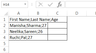
We could also have all the data in a single column with a fixed number of characters marking the segregation in the data.
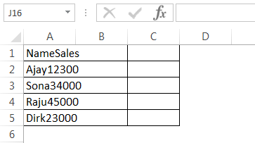
When data is received or arranged in any of the formats shown above, it becomes difficult to work with the data because it is not formatted into a proper row and column format. But if we see carefully, in the first screenshot, the columns (as it should be) are separated by semicolons – “;”, i.e. for the first row, the first column is the “First Name”, the second column is “Last Name”, and the third column is “Age”. Semicolons separate all the columns. This holds true for the rest of the rows. Therefore, we can split the data into a proper row and column format on the basis of the strategic delimiters in the data. Similarly, in the second screenshot, we see that all the data has been clubbed into a single column. However, upon closer observation, we see that the columns (as they should be) can be differentiated on the basis of their lengths.
The first column is “Name”, followed by “Sales”. We see that the length of “Name” is 4 and the length of “Sales” is 5. This holds true for all the rows in the table. Therefore, we can separate text data in excel into columns on the basis of their Fixed Lengths. With Excel, we have a solution to these kinds of problems. Two very useful features of Excel are the “Text to Columns” or the “Split Cell”, which helps to resolve these kinds of formatting issues by enabling data re-arrangement or data manipulation/cleaning since it becomes really difficult to work with a lot or all the data in a single column.
Note: There are several complicated formulae that can also achieve similar results, but they tend to be very convoluted and confusing. Text to Column is also much faster.
What is Text to Columns?
Typically, when we get the data from databases or from CSV or text sources, we encounter situations as shown above. We have a very handy feature in Excel called “Text to Columns” to resolve these kinds of problems.
It can be found in the Data tab and then in the “Data Tools” section.
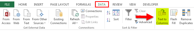
The shortcut from the keyboard is Alt+A+E. This will also open up the “Text to Columns” feature. Let us see some examples to understand how “Text to Columns” will solve our problem.
Examples of Separate text in Excel
Below are the different examples to separate text in excel:
Example #1
Split First Name, Last Name, and Age into separate text columns in excel (using delimiters) :
You can download this Separate text Excel Template here – Separate text Excel Template
Let us consider a situation where we have received the data in the following format.

We have “First Name”, “Last Name”, and “Age” data all clubbed into one column. Our objective is to split the data into separate text columns in excel.
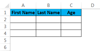
To split the data into separate text columns in excel, we need to follow the following steps:
Step1 – We will first select the data column:
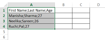
Step 2 – We will navigate to the “Data” tab and then go to the “Data Tools” section and click on “Text to Columns”.
This will open up the “Text to Columns” wizard.
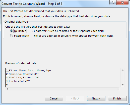
Step 3 – Now make sure that we click on “Delimited” to select it and then click on “Next”.
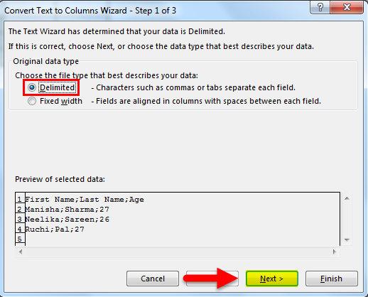
Step 4 – After this, in the next tab, deselect “Tab” first.
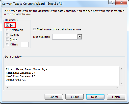
Then select “Semicolon” as the delimiter.
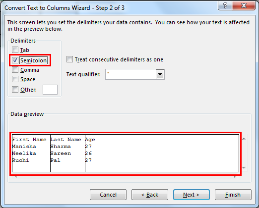
As soon as we select “Semicolon”, we see that the columns are now demarcated in the text preview. In the situation where there are multiple successive delimiters, we can choose to select the “Treat consecutive delimiters as one” option. Following that, we can click on the “Next” button.
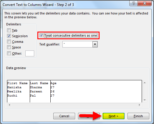
Step 5 – Next, we shall look at the section where the column data format is described. We can choose to keep the data as either :
- “General” – This converts numeric values to numbers, date values to dates, and remaining as text.
- “Text” – Converts all the values to text format.
- “Date” – Converts all the values to Date format (MDY, DMY, YMD, DYM, MYD, YDM)
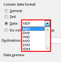
- Ignore Column – This will skip reading the column.
Next, we shall look at the “Advanced” option.
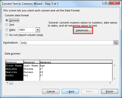
“Advanced” provides us with the option to choose the decimal separator and the thousands separator.
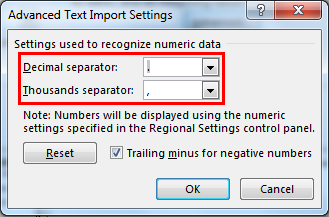
Next, we shall select the destination cell. Now, if we do not modify this, then it will overwrite the original column with “First Name”, the adjacent cell will become “Last Name”, and the cell adjacent to that will become “Age”. If we choose to keep the original column, we will need to mention a value here (which will be the next adjacent cell).
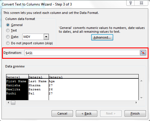
After this, we shall click on “Finish”.
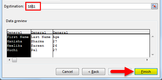
Our result will be as follows:
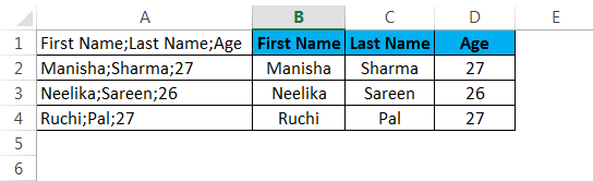
Example #2
Split Name, Sales into separate text columns in excel (using Fixed Width):
Suppose we have a scenario where we have data, as shown below.

As we can see, the entire data has been clubbed into one column (A). But here, we see that the format of the data is a bit different. We can make out that the first column (as it should be) is “Name” and the next column is “Sales”. “Name” has a length of 4, and “Sales” has a length of 5. Interestingly, all the names in the rows below also have a length of 4, and all the sales numbers have a length of 5. In this case, we can split the data from one column to multiple columns using “Fixed Width” since we do not have any delimiters here.
Step 1 – Select the column where we have the clubbed data.
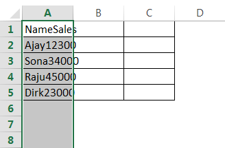
Step 2 – We will navigate to the “Data” tab and then go to the “Data Tools” section and click on “Text to Columns”.
This will open up the “Text to Columns” wizard.
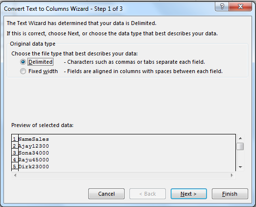
Step 3 – Now make sure that we click on “Fixed width” to select it and then click on “Next”.
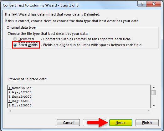
Step 4 – In the next screen, we shall have to adjust the fixed-width vertical divider lines (these are called Break Lines) in the Data Preview section.
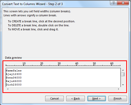
This can be adjusted as per user requirement.
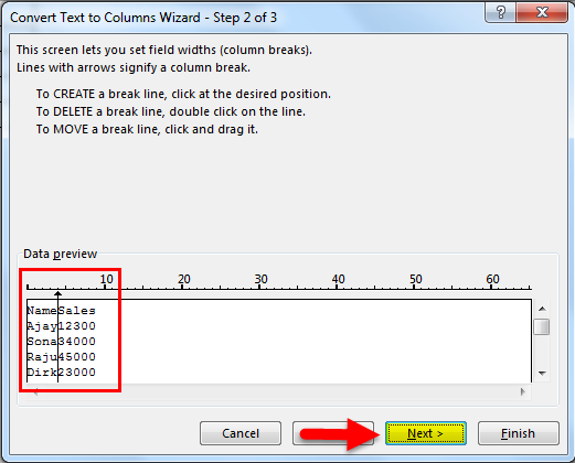
We need to click on the exact point where the first column width ends. This will bring the Break Line at that point.
Step 5 – Next, we shall look at the section where the column data format is described. We can choose to keep the data as either –
- “General” – This converts numeric values to numbers, date values to dates and remaining as text.
- “Text” – Converts all the values to text format.
- “Date” – Converts all the values to Date format (MDY, DMY, YMD, DYM, MYD, YDM)
- Ignore Column – This will skip reading the column.
Next, we shall look at the “Advanced” option.
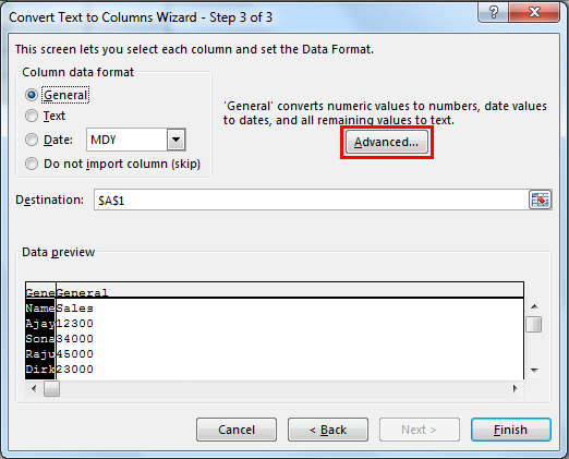
“Advanced” provides us with the option to choose the decimal separator and the thousands separator.
Next, we shall select the destination cell. If we do not modify this, it will overwrite the original column with “Name”; the adjacent cell will become “Sales”. If we choose to keep the original column, we will need to mention a value here (which will be the next adjacent cell).
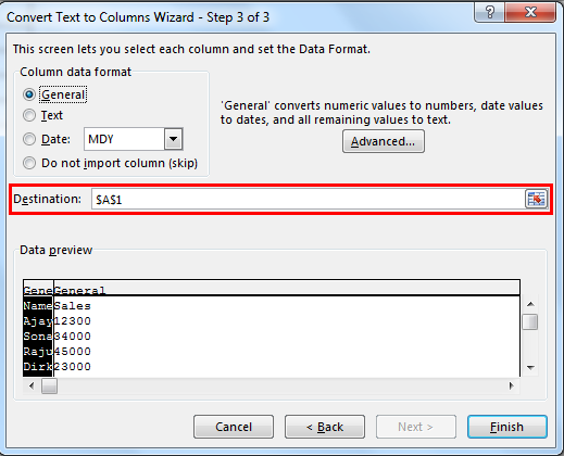
After this, we shall click on “Finish”.
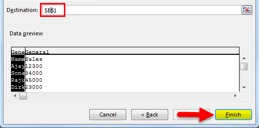
Our result will be as follows:
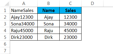
We can use the same logic to extract the first “n” characters from a data column as well.
Things to Remember about Separate text in Excel
- We should stop using complicated formulae and/or copy-paste to split a column (separate the clubbed data from a column) and start using Text to Columns.
- In the Fixed-Width method, Excel will split the data based on the character length.
- In the Delimited method, Excel will split the data based on a set of delimiters such as comma, semicolon, tab etc.
- Easily access Text to Columns by using the Keyboard shortcut – Alt+A+E.
Recommended Articles
This has been a guide to Separate text in Excel. Here we discuss the Separate text in Excel and how to use the Separate text in Excel along with practical examples and a downloadable excel template. You can also go through our other suggested articles –
- Excel Text with Formula
- Search For Text in Excel
- Formatting Text in Excel
- VBA Text
When working in Microsoft Excel, you may encounter a situation where a cell’s text is all jumbled up. Such a cell will contain numbers and texts, making it hard to decipher what it means. It mostly happens when importing data from other systems that your Excel program cannot read. Such a scenario can be so frustrating and time-consuming. To solve this scenario, it is advisable to separate the texts and numbers for your worksheet to make sense and be easily understandable. Excel has a lot of features that help make this possible.
In the article below, we will show you different methods you can take when you want to separate numbers and texts in Excel. Let’s get started.
Method 1: Using the Flash Fill feature to separate texts and numbers in Excel
1. In your open Excel workbook, select the cell that contains the numbers and texts you want to separate.

2. In the adjacent blank cell, type in the characters of your first text string.

3. Select all the cell ranges where you want to fill the numbers, and click the Data tab on the main menu ribbon.

4. Select the Flash Fill option, and only the numbers will be filled in these cells.

All the text will be separated

5. In another column, one adjacent to the separated number column, type in the first number of the string

6. Select all the cells below the first entry, and click Data> Flash Fill. Doing so will separate the numbers from the string.

Method 2: separating numbers and texts using formulas
You can easily separate your numbers from texts using Excel formulas. It may require the use of complex formulas, but the method is reliable. When it comes to separating texts, we use RIGHT, LEFT, MID, and other text functions. For this to be successful, a user has to know the exact number and texts to extract
The formula to use is =MIN(FIND({0, 1, 2, 3, 4, 5, 6, 7, 8, 9}, a2& «0123456789»))
So long as you understand the FIND function, the formula is pretty much easy to grasp. The function will run ten times, once for each number, and the MIN function will return the first number in the cell. Let’s use the following data as an example
1. To extract the names, enter this formula into a blank cell where you want to place the results =LEFT(A2,MIN(FIND({0, 1, 2, 3, 4, 5, 6, 7, 8, 9},A2& «0123456789»))-1)
2. To extract the numbers, enter this formula into a black cell that will hold the results =RIGHT(A2,LEN(A2)-MIN(FIND({0, 1, 2, 3, 4, 5, 6, 7, 8, 9},A2& «0123456789»))+1) , (A2 IS THE CELL WHICH CONTAINS THE TEXT STRING YOU WANT TO SEPARATE)
3. After filling up these formulas press the Enter key, and the texts and numbers will separate.
4. To separate the other text and number strings, select the first two separated cells and drag the fill handle.
Method 3: separating irregularly mixed texts and numbers using VBA code
1. Hold down the Alt + F11 keys to open the VBA editor window.
2. Click insert and select Module. In the open Module window, paste or type in your code. For example, you can use the code below to separate texts and numbers into different cells from one cell.
Option Explicit

Public Function Strip(ByVal x As String, LeaveNums As Boolean) As Variant

Dim y As String, z As String, n As Long

For n = 1 To Len(x)

y = Mid(x, n, 1)

If LeaveNums = False Then

If y Like "[A-Za-z ]" Then z = z & y 'False keeps Letters and spaces only

Else

If y Like "[0-9. ]" Then z = z & y 'True keeps Numbers and decimal points

End If

Next n

Strip = Trim(z)

End Function
3. Save and close the code window to return to your worksheet. In a blank cell, enter the formula =Strip(A2,FALSE) to extract the text string only. Drag the fill handle to the cells you want to fill.
4. In another blank cell, type in the formula =NUMBERVALUE(Strip(A2,TRUE)) . Drag the fill handle downwards to other cells to fill in only the numbers.
Note that, while using this method, the result may be incorrect when there are any decimal numbers in your text string.
This tutorial will demonstrate how to split text strings using a space, comma and more in Excel and Google Sheets.
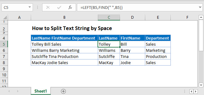
Split Text String with Text to Columns
You can split a text string with the Text to Columns feature in Excel.
Select the text you wish to split.
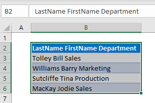
In the Ribbon, select Data>Text to Columns.
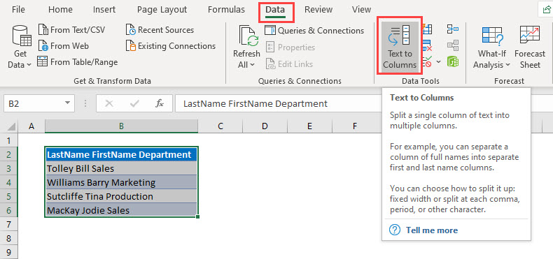
Keep the option “Delimited” selected and click Next.
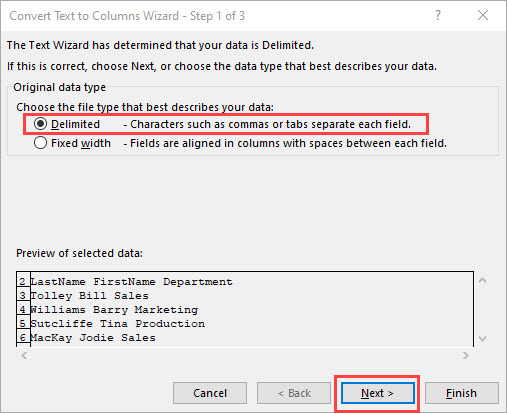
Select “Space” as the Delimiter, and amend the Text qualifier to “None”
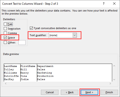
Click Next.
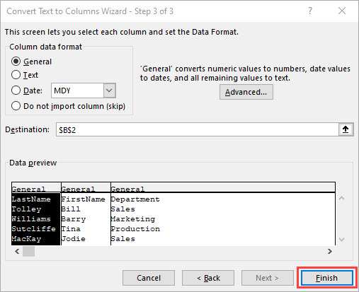
In this step, you can change the data type of the column. Leave them as they are and click Finish.
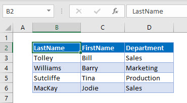
Split Text String by Space
To split a text string at a space or comma, we can use the FIND, LEFT, MID and RIGHT functions.
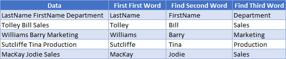
LEFT and FIND Functions
First, we can find the LastName by using the LEFT and FIND functions.
=LEFT(B3, FIND(" " , B3))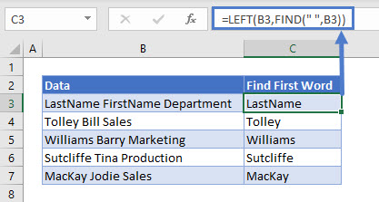
MID and FIND Functions
We can then use the MID and FIND Functions to find the second word in the text string.
=MID(B3,FIND(" ",B3),FIND(" ",B3,FIND(" ",B3)+1)-FIND(" ", B3))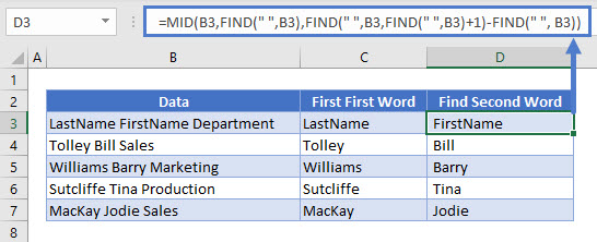
RIGHT and FIND Functions
Finally, we can use the RIGHT, LEN and FIND Functions to find the third word in the text string.
=RIGHT(B3, LEN(B3)-FIND(" ", B3,FIND(" ",B3)+1))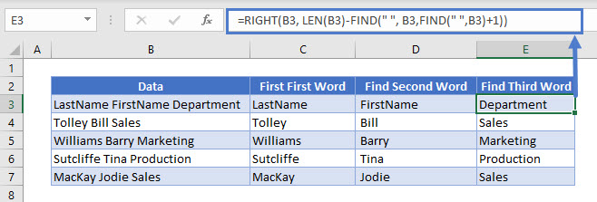
Split Text String by Comma or Other Character
You can use the same formulas to find commas or any other characters in a text string and split the text string accordingly.
The formulas would be slightly different
Find the First word
=LEFT(B3,FIND(",",B3)-1)To find the second word
=MID(B3,FIND(",",B3)+1,FIND(",",B3,FIND(",",B3)+1)-FIND(",", B3)-1)To find the third word
=RIGHT(B3, LEN(B3)-FIND(",", B3,FIND(",",B3)+1)-1)Split Text String with Text to Columns in Google Sheets
Google sheets also has a Text to Columns feature.
Select the text you wish to split, and then click on the Data menu > Split text to columns.
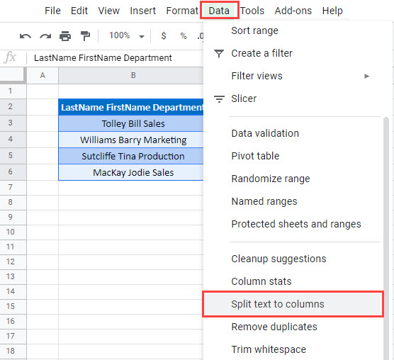
Click on Detect Automatically
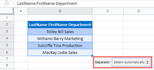
Select the Space.
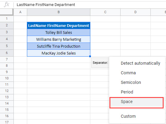
Your text will be split into columns.
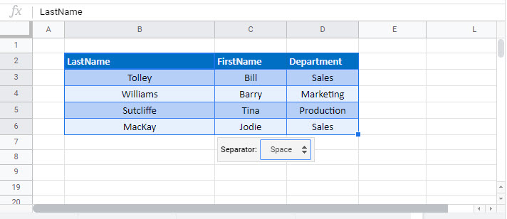
Split Text String by Comma or Other Character
You can use the FIND, LEFT, MID and RIGHT functions in Google Sheets as you do in Excel to split the text.
The formulas to extract the data for the LastName, FirstName and Department Columns are the same ones that are used in Excel.
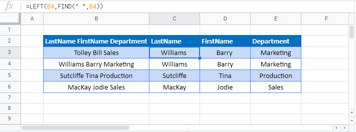
-
Excel 365
-
Excel 2021
-
Excel 2019
-
Excel 2016
-
February 12, 2022 -
12 Comments
You’ll sometimes encounter a situation where a cell contains both text and numbers, often when data has been imported from another system.
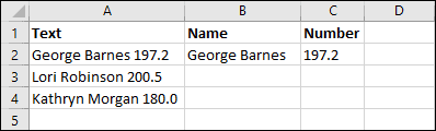
In this example, you want to separate the names and numbers from column A into columns B and C. There are three ways that you could do this.
Option 1: Flash Fill
Flash Fill was a feature introduced in Excel 2013. If you have an older version or a Mac version you won’t be able to use it.
Flash Fill makes this extremely easy, and it’s almost always the best choice for tasks like this.
To use Flash Fill you first need to provide it with an example of what you are trying to do, as shown above. Once you’ve provided an example, click:
Home > Editing > Fill > Flash Fill
You can also use the shortcut key <Ctrl>+<E> to do this.
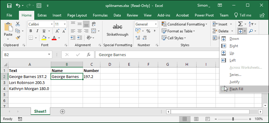
Flash Fill looks at your example, figures out what you are trying to do, and automatically extracts all of the other names.
You can repeat the same process for column C and all of the names and numbers are extracted!
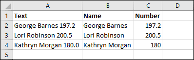
Flash Fill is explained in more depth in our Essential Skills course, along with some more advanced Flash Fill techniques.
Flash Fill offers the simplest and easiest solution, but it needs to be done manually each time you need to split the names and won’t be available to you if you are using a Mac version of Excel or an older version of Excel for Windows.
Option 2: Text to Columns
If you’re an experienced Excel user, the Text to Columns feature might also have come to mind. Text to Columns allows you to split cells like this, but only if they are separated by a consistent character or a fixed width.
In this case, Text to Columns could be used to split the data using a space as the delimiter. This would result in 3 columns rather than the two you want, so you would need to then concatenate the names back together.
You can access the Text to Columns tool by clicking: Data > Data Tools > Text to Columns
Using Text to Columns is covered in depth in our Expert Skills course.
Option 3: Using Formulas
The previous options only offer a ‘one-off’ solution. If the data in column A came from an external data source, you wouldn’t want to have to re-run Flash Fill or Text to Columns every time you refreshed the data.
It’s possible to extract the names and numbers using formulas, but you’ll need some very complex formulas to do this.
Finding the position of the first number
The first thing your formula will need to do is find the position of the first number in the cell. The formula to do this is:
=MIN(FIND({0,1,2,3,4,5,6,7,8,9},A2&”0123456789″))
This looks daunting, but it’s not actually that hard to understand if you understand the FIND function. FIND is covered in depth in our Expert Skills course.
The {0,1,2,3,4,5,6,7,8,9} numbers in curly brackets might also look confusing. This is called an ‘array’. What is means is that the FIND function will run 10 times, once for each of the numbers. The MIN function will then return the lowest value that is returned (i.e. the position of the first number in the cell).
The reason you’re concatenating the text “0123456789” is because the FIND function will return an error if it doesn’t find what it’s searching for, and this will prevent the MIN function from being able to return a result. To make sure that FIND can always return a valid result each time it runs, you append all of the numbers to the end of the text it is searching.
Extracting the names
Now that you have the position of the first number, you can use the LEFT function to extract the names like this:
=LEFT(A2,MIN(FIND({0,1,2,3,4,5,6,7,8,9},A2&”0123456789″))-1)
The LEFT function is explained in depth in our Expert Skills course.
Extracting the numbers
In a very similar way, the numbers can be extracted using the RIGHT and LEN functions like this:
=RIGHT(A2,LEN(A2)-MIN(FIND({0,1,2,3,4,5,6,7,8,9},A2&”0123456789″))+1)
As with LEFT, the RIGHT and LEN functions are covered in our Expert Skills course.
The Result
After filling down the formulas you can see that they have successfully extracted the names and numbers. These formulas will work in any version of Excel, and will continue to work even if the data in column A changes.
You can download a copy of the workbook showing the formulas in action.


These are the only up-to-date Excel books currently published and includes the new Dynamic Arrays features.
They are also the only books that will teach you absolutely every Excel skill including Power Pivot, OLAP and DAX.
Some of the things you will learn
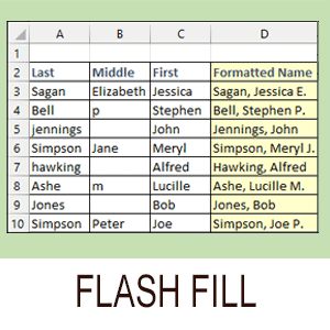

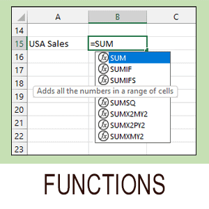
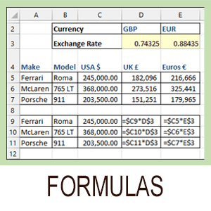

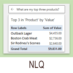


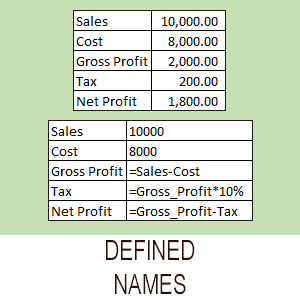


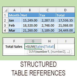
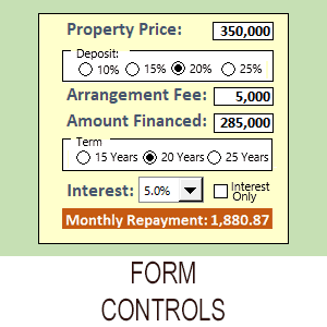
Share this article
Recent Articles
12 Responses
-
Based on the above advice, it cannot separate text and numbers when numbers are in front of the text, e.g. 12345abcde. Any further advice?
-
Hi Alex,
All of the above solutions should work with the numbers in front of the text.
For the formula-based approach the difference would be that you would need to search for the last number rather than the first. You could do this by using the MAX function instead of the MIN function.
Once you have the location of the last number you should be able to use the LEFT function to extract all of the numbers.-
ACTUALLY THIS IS NOT WORKING FOR ME.
-
If you can be more specific about what you are trying to do and how it is not working I should be able to offer some advice.
-
After copying the formula for finding the first numeral, edit the double quote marks in the copy, replacing each of them with your keyboard’s double quote key.
This is a common problem on websites: the articles are written with word processing software which will replace the keyboard typed double quotes with slicker ones (in Word this is called using smart quotes) meant for publishing. And if that does not happen, or is correctly fixed afterward, any processing when loading to the webiste may do it also.
-
-
I also have a situation where I need to separate numbers and text in the same cell, where the numbers are in front. I tried using the MAX function and it’s not working for me. What formula could I use to create the result below?
Before: 00868#09ALVARADO
After: 00868#09 ALAVARADO <—There’s a space between «9» and «A»-
If the two codes have a consistent length you should be able to do this easily using Flash Fill or by using Text To Columns, as mentioned above. If you need a formula-based solution and the codes are always the same length you should also be able to do this easily using the LEFT and RIGHT functions. It’s only in cases where the codes could have a variable length that you will need a formula that searches for the position of the last number or first letter of the code.
The MAX solution will only work correctly if all of the numbers 0-9 can be found in the target, so it might not actually be the best approach in a situation like this. Formulas do exist that can reliably extract the last number from a value without any foreknowledge of what numbers might be present, but they are much more complex.
A simpler solution in this case would be to find the first letter instead of the last number. Assuming the value is in cell A2, you could do that using:
=MIN(FIND({“A”,”B”,”C”,”D”,”E”,”F”,”G”,”H”,”I”,”J”,”K”,”L”,”M”,”N”,”O”,”P”,”Q”,”R”,”S”,”T”,”U”,”V”,”W”,”X”,”Y”,”Z”},A2&”ABCDEFGHIJKLMNOPQRSTUVWXYZ”))-1This works in exactly the same way as the formula above, but it runs the FIND function 26 times (once for each letter of the alphabet) and returns the lowest result. You can then extract the values on each side using the LEFT, RIGHT and LEN functions.
To get the part before the A you would use:
=LEFT(A2,MIN(FIND({“A”,”B”,”C”,”D”,”E”,”F”,”G”,”H”,”I”,”J”,”K”,”L”,”M”,”N”,”O”,”P”,”Q”,”R”,”S”,”T”,”U”,”V”,”W”,”X”,”Y”,”Z”},A2&”ABCDEFGHIJKLMNOPQRSTUVWXYZ”))-1)To get the part after the A you would use:
=RIGHT(A2,LEN(A2)-(MIN(FIND({“A”,”B”,”C”,”D”,”E”,”F”,”G”,”H”,”I”,”J”,”K”,”L”,”M”,”N”,”O”,”P”,”Q”,”R”,”S”,”T”,”U”,”V”,”W”,”X”,”Y”,”Z”},A2&”ABCDEFGHIJKLMNOPQRSTUVWXYZ”)))-1)Now that you have extracted both parts of the value, you could join them back together with a space between them using the & operator, for example:
=B2&” “&C2
-
-
-
-
Could you please help to find highest value and lowest value from this
please paste the below data in one cell (Ex. A1) and need to find highest valueCell: A1
a)63Ra b)64Ra c)65Ra d)62Ra e)61Ra f)63Ra g)60Ra h)62Ra-
Hi Adaikkala,
I would recommend first breaking each of the items into separate cells, either using Flash Fill or the Text to Columns feature. You can see how to use Flash Fill above, and Text to Columns is covered in this article.
Both skills are covered in depth in our courses.
After the values have been placed in separate cells you should be able to use the skills shown above to extract the numbers and could then use the MAX and MIN functions to determine the highest and lowest.
-
-
Thank you very much
-
=MIN(FIND({0,1,2,3,4,5,6,7,8,9},A2&”0123456789″))
does nothing for me
i tried replacing ” and ; etc even typed it by hand new and it does not work.
the line always just says
=MIN(FIND({0,1,2,3,4,5,6,7,8,9},A2&”0123456789″))
instead of showing the result.
Any thoughts how to fix this?-
I’ve just tested this and it worked perfectly for me. With the text “George Barnes 197.2″ in cell A2, the formula: =MIN(FIND({0,1,2,3,4,5,6,7,8,9},A2&”0123456789”)) returned 15 as expected. If you copy and paste from the web page you’ll have to manually re-enter the double quotation marks (web page quotes are different to Excel quotes) but you’ve said that you’ve done that.
My best guess is that it is an Excel version issue. There have been a huge number of Excel versions and some have bugs that others don’t have, some also have functions that others don’t have. All I can report is that it worked perfectly using Excel 365 version 2103 Build 13901.20462 which was the latest version of Excel at time of writing. Having said that, I’d also expect it to work on all other versions of Excel but your experience suggests otherwise!
-
Leave a Reply
Bottom Line: Learn how to use formulas and functions in Excel to split full names into columns of first and last names.
Skill Level: Intermediate
Watch the Tutorial
Download the Excel Files
You can download both the before and after files below. The before file is so you can follow along, and the after file includes all of the formulas already written.
Splitting Text Into Separate Columns
We’ve been talking about various ways to take the text that is in one column and divide it into two. Specifically, we’ve been looking at the common example of taking a Full Name column and splitting it into First Name and Last Name.
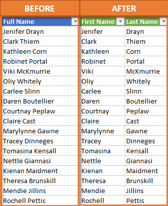
The first solution we looked at used Power Query and you can view that tutorial here: How to Split Cells and Text in Excel with Power Query. Then we explored how to use the Text to Columns feature that’s built into Excel: Split Cells with Text to Columns in Excel. Today, I want to show you how to accomplish the same thing with formulas.
Using 4 Functions to Build our Formulas
To split our Full Name column into First and Last using formulas, we need to use four different functions. We’ll be using SEARCH and LEFT to pull out the first name. Then we’ll use LEN and RIGHT to pull out the last name.
The SEARCH Function
They key to breaking up the first names from the last names is for Excel to identify what all of the full names have in common. That common factor is the space character that separates the two names. To help our formula identify everything to the left of that space character as the first name, we need to use the SEARCH function.
The SEARCH function returns the number of the character at which a specific character or text string is found, reading left to right. In other words, what number is the space character in the line of characters that make up a full name? In my name, Jon Acampora, the space character is the 4th character (after J, o, and n), so the SEARCH function returns the number 4.
There are three arguments for SEARCH.
- The first argument for the SEARCH function is find_text. The text we want to find in our entries is the space character. So, for find_text, we enter ” “, being sure to include the quotation marks.
- The second argument is within_text. This is the text we are searching in for the space character. That would be the cell that has the full name. In our example, the first cell that has a full name is A2. Since we are working with Excel Tables, the formula will copy down and change to B2, C2, etc., for each respective row.
- The third and last argument is [start_num]. This argument is for cases where you want to ignore a certain number of characters in the text before beginning your search. In our case, we want to search the entire text, beginning with the very first character, so we do not need to define this argument.
All together, our formula reads: =SEARCH(” “,A2)
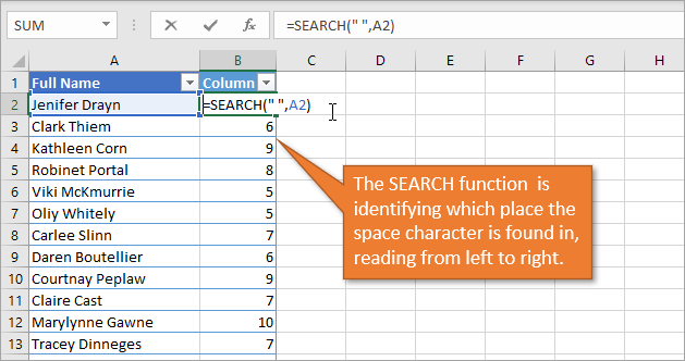
I started with the SEARCH function because it will be used as one of the arguments for the next function we’re going to look at. That is the LEFT function,
The LEFT Function
The LEFT function returns the specified number of characters from the start of a text string. To specify that number, we will use the value we just identified with the SEARCH function. The LEFT function will pull out the letters from the left of the Full Name column.
The LEFT function has two arguments.
- The first argument is text. That is just the cell that the function is pulling from—in our case A2.
- The second argument is [num_chars]. This is the number of characters that the function should pull. For this argument, we will use the formula we created above and subtract 1 from it, because we don’t want to actually include the space character in our results. So for our example, this argument would be SEARCH(” “,A2)-1
All together, our formula reads =LEFT(A2,SEARCH(” “,A2)-1)
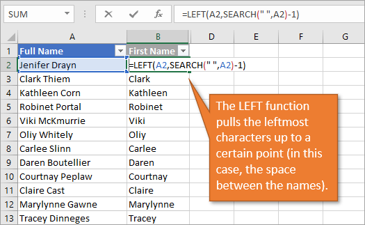
Now that we’ve extracted the first name using the LEFT function, you can guess how we’re going to use the RIGHT function. It will pull out the last name. But before we go there, let me explain one of the components that we will need for that formula. That is the LEN function.
The LEN Function
LEN stands for LENGTH. This function returns the number of characters in a text string. In my name, there are 12 characters: 3 for Jon, 8 for Acampora, and 1 for the space in between.
There is only one argument for LEN, and that is to identify which text to count characters from. For our example, we again are using A2 for the Full Name. Our formula is simply =LEN(A2)
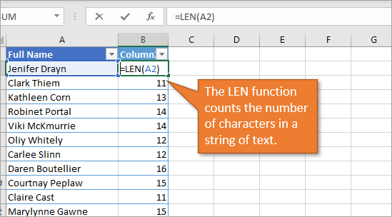
The RIGHT Function
The RIGHT formula returns the specified number of characters from the end of a text string. RIGHT has two arguments.
- The first argument is text. This is the text that it is looking through in order to return the right characters. Just as with the LEFT function above, we are looking at cell A2.
- The second argument is [num_chars]. For this argument we want to subtract the number of characters that we identified using the SEARCH function from the total number of characters that we identified with the LEN function. That will give us the number of characters in the last name.
Our formula, all together, is =RIGHT(A2,LEN(A2)-SEARCH(” “,A2))
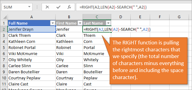
Note that we did not subtract 1 like we did before, because we want the space character included in the number that is being deducted from the total length.
Pros and Cons for Using Formulas to Split Cells
The one outstanding advantage to this method for splitting text is the automatic updates. When edits, additions, or deletions are made to the Full Name column, the First and Last names change as well. This is a big benefit compared to using Text to Columns, which requires you to completely repeat the process when changes are made. And even the Power Query method, though much simpler to update than Text to Columns, still requires a refresh to be manually selected.
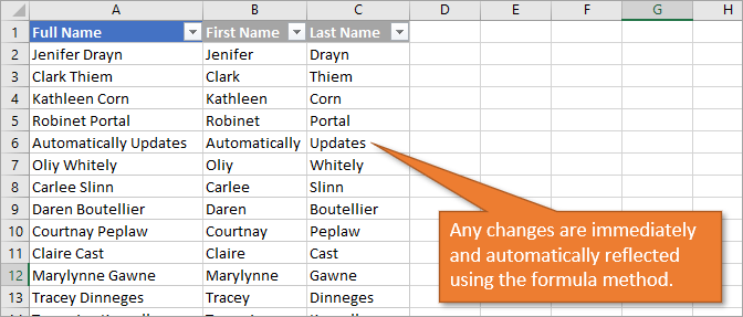
Of course, one obvious disadvantage to this technique is that even though each of the four functions are relatively simple to understand, it takes some thought and time to combine them all and create formulas that work correctly. In other words, is not the easiest solution to implement of the three methods presented thus far.
Another disadvantage to consider is the fact that this only works for scenarios that have two names in the Full Name column. If you have data that includes middle names or two first names, the formula method isn’t helpful without making some considerable modifications to the formulas. (Homework challenge! If you’d like to give that a try, please do so and let us know your results in the comments.) As we saw in the Power Query tutorial, you do in fact have the capability to pull out more than two names with that technique.
Here are the links to the other posts on ways to split text:
- Split Cells with Text to Columns in Excel
- How to Split Text in Cells with Flash Fill in Excel
- How to Split Cells and Text in Excel with Power Query
- Split by Delimiter into Rows (and Columns) with Power Query
Conclusion
I hope you’ve learned something new from this post and that is helpful as you split data into separate columns. If you have questions or remarks, please leave a comment below!