
Sometimes you may have the text and numeric data in the same cell, and you may have a need to separate the text portion and the number portion in different cells.
While there is no inbuilt method to do this specifically, there are some Excel features and formulas you can use to get this done.
In this tutorial, I will show you 4 simple and easy ways to separate text and numbers in Excel.
Let’s get to it!
Separate Text and Numbers Using Flash Fill
Below I have the employee data in column A, where the first few alphabets indicate the department of the employee and the numbers after it indicates the employee number.

From this data, I want to separate the text part and the number part and get these into two separate columns (columns B and C).
The first method that I want to show you to separate text and numbers in Excel is by using Flash Fill.
Flash Fill (introduced in Excel 2013) works by identifying patterns based on user input.
So if I manually enter the expected result in column B, Flash Fill will try and decipher the pattern and give me the result for all the cells in that column.
Below are the steps to separate the text part from the cell and get it in column B:
- Select cell B2
- Manually enter the expected result in cell B2, which would be MKT

- With cell B2 selected, place the cursor at the bottom right part of the selection. You’ll notice that the cursor changes into a plus icon (this is called Fill Handle)

- Hold the left mouse/trackpad key and drag the Fill Handle to fill the cells. Don’t worry if the cells are filled with the same text
- Click on the Auto Fill Options icon and then select the ‘Flash Fill’ option

The above steps would extract the text part from the cells in column A and give you the result in column B.

Note that in some cases, Flash Fill may not be able to identify the right pattern. In such cases, it would be best to enter the expected result in two or three cells, use the Fill Handle to fill the entire column, and then use Flash Fill on this data.
You can follow the same process to extract the numbers in column C. All you need to do is enter the expected result in cell C2 (step 2 in the process laid out above)
Note that the result you get from Flash Fill is static and would not update in case you change the original data in column A. If you want the result to be dynamic, you can use the formula method covered next.
Separate Text and Numbers Using Formula
Below I have the employee data in column A and I want to use a formula to extract only the text part and put it in column B and extract the number part and put it in column C.
Since the data is not consistent (i.e., the alphabets in the department code and the numbers in the employee number are not of the consistent length), I cannot use the LEFT or RIGHT function to extract only the text portion or only the number portion.
Below is the formula that will extract only the text portion from the left:
=LEFT(A2,MIN(IFERROR(FIND({0,1,2,3,4,5,6,7,8,9},A2),""))-1)

And below is the formula that will extract all the numbers from the right:
=MID(A2,MIN(IFERROR(FIND({0,1,2,3,4,5,6,7,8,9},A2),"")),100)

How does this formula work?
Let me first explain the formula that we use to separate the text part on the left.
=LEFT(A2,MIN(IFERROR(FIND({0,1,2,3,4,5,6,7,8,9},A2),””))-1)
The FIND part in the formula finds the position of digits 0 to 9 in cell A2. In case it finds that digit in cell A2, it returns the position of that digit, and in case it is not able to find that digit, then it returns the value error (#VALUE!)
For cell A2, it gives a result as shown below:
{#VALUE!,4,#VALUE!,#VALUE!,#VALUE!,6,#VALUE!,5,#VALUE!,#VALUE!}
- For 0, it returns #VALUE! as it cannot find this digit in cell A2
- For 1, it returns 4 as that is the position of the first occurrence of 1 in cell A2
- and so on…
This FIND formula is then wrapped inside the IFERROR function, which removes all the value errors but leaves the numbers.
The result of it looks like as shown below:
{“”,4,””,””,””,6,””,5,””,””}
The MIN function then goes through the above result and gives us the minimum value from the results. Since each number in the array represents the position of that corresponding number, the minimum value tells us where the numerical value starts in the cell.
Now that we know where the numerical values start, I have used the LEFT function to extract everything before this position (which would be all the text in the cell).
Similarly, you can use the same formula with a minor tweak to extract all the numbers after the text. To extract the numbers, where we know the starting position of the first digit, use the MID function to extract everything starting from that position.
And what if the situation is reversed – where we have the numbers first and the text later and we want to separate the numbers and text?
You can still use the same logic with one minor change – instead of finding the minimum value that gives us the position of the 1st digit in the cell, you need to use the MAX function To find the position of the last digit in this cell. Once you have it, you can again use the LEFT function or the MID function to separate the numbers and text.
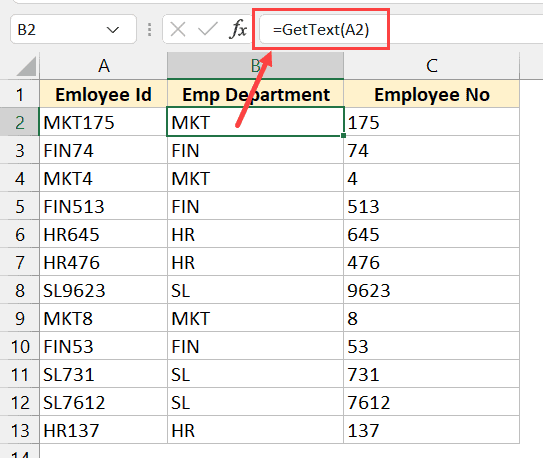
Separate Text and Numbers Using VBA (Custom Function)
While you can use the formulas shown above to separate the text and numbers in a cell and extract these into different cells – if this is something you need to do quite often, you also have the option to create your own custom function using VBA.
The benefit of creating your own function would be that it would be a lot easier to use (with just one function that takes only one argument).
You can also save this custom function VBA code into the Personal Macro Workbook so that it would be available in all your Excel workbooks.
Below the VBA code that could create a function ‘GetNumber’ that would take the cell reference as the input argument, extract all the numbers in the cell, and give it as the result.
'Code created by Sumit Bansal from https://trumpexcel.com
'This code will create a function that can separate numbers from a cell
Function GetNumber(CellRef As String)
Dim StringLength As Integer
StringLength = Len(CellRef)
For i = 1 To StringLength
If IsNumeric(Mid(CellRef, i, 1)) Then Result = Result & Mid(CellRef, i, 1)
Next i
GetNumber = Result
End Function
And below the VBA code that would create another function ‘GetText’ that would take the cell reference as the input argument and give you all the text from that cell
'Code created by Sumit Bansal from https://trumpexcel.com
''This code will create a function that can separate text from a cell
Function GetText(CellRef As String)
Dim StringLength As Integer
StringLength = Len(CellRef)
For i = 1 To StringLength
If Not (IsNumeric(Mid(CellRef, i, 1))) Then Result = Result & Mid(CellRef, i, 1)
Next i
GetText = Result
End Function
Below are the steps to add this code to your excel workbook so that this function becomes available for you to use in the worksheet:
- Click the Developer tab in the ribbon
- Click on the Visual Basic icon

- In the Visual Basic editor that opens up, you would see the Project Explorer on the left. This would have the workbook and the worksheet names of your current Excel workbook. If you don’t see this, click on the View option in the menu and then click on Project Explorer

- Select any of the sheet names (or any object) for the workbook in which you want to add this function
- Click on the Insert option in the top toolbar and then click on Module. This will insert a new module for that workbook

- Double click on the module icon in ‘Project Explorer’. This will open the module code window.

- Copy and paste the above custom function code into the module code window

- Close the VB Editor
With the above steps, we have added the custom function code to the Excel workbook.
Now you can use the functions =GETNUMBER or =GETTEXT just like any other worksheet function.
Note – Once you have the macro code in the module code window, you need to save the file as a Macro Enabled file (with the .xlsm extension instead of the .xlsx extension)
If you often have a need to separate text numbers from cells in Excel, it would be more efficient if you copy these VBA codes for creating these custom functions, and save these in your Personal Macro Workbook.
You can learn how to create and use Personal Macro Workbook in this tutorial I created earlier.
Once you have these functions in the Personal Macro Workbook, you would be able to use these on any Excel workbook on your system.
One important thing to remember when using functions that are stored in Personal Macro Workbook – you need to prefix the function name with =PERSONAL.XLSB!. For example, if I want to use the function GETNUMBER in a workbook in Excel, and I have saved the code for it in the postal macro workbook, I will have to use =PERSONAL.XLSB!GETNUMBER(A2)
Separate Text and Numbers Using Power Query
Power Query is slowly becoming my favorite feature in Excel.
If you’re already using Power Query as a part of your workflow, and you have a data set where you want to separate the text and numbers into separate columns, Power Query will do it in a few clicks.
When you have your data in Excel and you want to use Power Query to transform that data, one prerequisite is to convert that data into an Excel Table (or a named range).
Below I have an Excel Table that contains the data where I want to separate the text and number portions into separate columns.

Here are the steps to do this:
- Select any cell in the Excel Table
- Click the Data tab in the ribbon

- In the Get and Transform group, click on the ‘From Table/Range’

- In the Power Query editor that opens up, select the column from which you want to separate the numbers and text
- Click the Transform tab in the Power Query ribbon

- Click on the Split Column option

- Click on ‘By Non Digit to Digit’ option.

- You’ll see that the column has been split into two columns where one has only the text and the other only has the numbers

- [Optional] Change the column names if you want
- Click the Home tab and then click on Close and Load. This will insert a new sheet and give us the output as an Excel Table.

The above steps would take the data from the Excel Table we originally had, use Power Query to split the column and separate the text and the number parts into two separate columns, and then give us back the output in a new sheet in the same workbook.

Note that we used the option ‘By Non-Digit to Digit’ option in step 7, which means that every time there is a change from a non-digit character to a digit, a split would be made. If you have a dataset where the numbers are first followed by text, you can use the ‘By Digit to Non-Digit’ option
Now let me tell you the best part about this method. Your original Excel Table (which is the data source) is connected to the output Excel Table.
So if you make any changes in your original data, you don’t need to repeat the entire process. You can simply go to any cell in the output Excel Table, right click and then click on Refresh.
Power query would run in the back end, check the entire original data source, do all the transformations that we did in the steps above, and update your output result data.
This is where Power Query really shines. If there is a set of transformations that you often need to do on a data set, you can use Power Query to do that transformation once and set the process. Excel would create a connection between the original data source and the resulting output data and remember all the steps you had taken to transform this data.
Now, if you get a new data set you can simply put it in the place of your original data and refresh the query, and you will get the result in a few seconds. Alternatively, you can simply change the source in Power Query from the existing Excel table to some other Excel Table (in same or different workbook).
So these are four simple ways you can use to separate numbers and text in Excel. if this is a once-in-a-while activity, you’re better off using Flash Fill or the formula method.
And in case this is something you need to do quite often, then I would suggest you consider the VBA method where we created a custom function or the Power Query method.
I hope you found this Excel tutorial useful.
Other Excel tutorials you may also like:
- Separate First and Last Name in Excel (Split Names Using Formulas)
- How to Convert Numbers to Text in Excel
- Convert Text to Numbers in Excel – A Step By Step Tutorial
- How to Compare Text in Excel
- How to Quickly Combine Cells in Excel
- How to Combine First and Last Name in Excel
- How to Extract the First Word from a Text String in Excel (3 Easy Ways)
- Extract Numbers from a String in Excel (Using Formulas or VBA)
- How to Extract a Substring in Excel (Using TEXT Formulas)
-
Excel 365
-
Excel 2021
-
Excel 2019
-
Excel 2016
-
February 12, 2022 -
12 Comments
You’ll sometimes encounter a situation where a cell contains both text and numbers, often when data has been imported from another system.
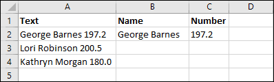
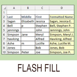
In this example, you want to separate the names and numbers from column A into columns B and C. There are three ways that you could do this.
Option 1: Flash Fill
Flash Fill was a feature introduced in Excel 2013. If you have an older version or a Mac version you won’t be able to use it.
Flash Fill makes this extremely easy, and it’s almost always the best choice for tasks like this.
To use Flash Fill you first need to provide it with an example of what you are trying to do, as shown above. Once you’ve provided an example, click:
Home > Editing > Fill > Flash Fill
You can also use the shortcut key <Ctrl>+<E> to do this.
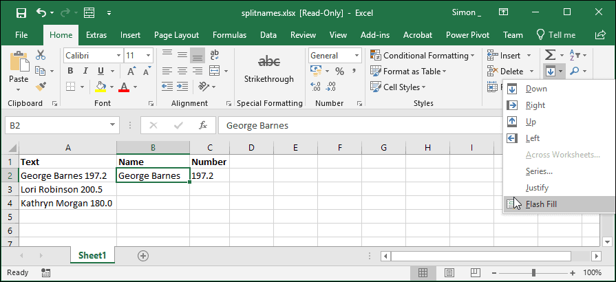
Flash Fill looks at your example, figures out what you are trying to do, and automatically extracts all of the other names.
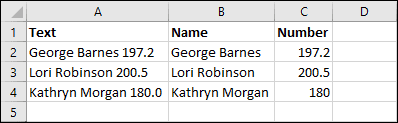
You can repeat the same process for column C and all of the names and numbers are extracted!
Flash Fill is explained in more depth in our Essential Skills course, along with some more advanced Flash Fill techniques.
Flash Fill offers the simplest and easiest solution, but it needs to be done manually each time you need to split the names and won’t be available to you if you are using a Mac version of Excel or an older version of Excel for Windows.
Option 2: Text to Columns
If you’re an experienced Excel user, the Text to Columns feature might also have come to mind. Text to Columns allows you to split cells like this, but only if they are separated by a consistent character or a fixed width.
In this case, Text to Columns could be used to split the data using a space as the delimiter. This would result in 3 columns rather than the two you want, so you would need to then concatenate the names back together.
You can access the Text to Columns tool by clicking: Data > Data Tools > Text to Columns
Using Text to Columns is covered in depth in our Expert Skills course.
Option 3: Using Formulas
The previous options only offer a ‘one-off’ solution. If the data in column A came from an external data source, you wouldn’t want to have to re-run Flash Fill or Text to Columns every time you refreshed the data.
It’s possible to extract the names and numbers using formulas, but you’ll need some very complex formulas to do this.
Finding the position of the first number
The first thing your formula will need to do is find the position of the first number in the cell. The formula to do this is:
=MIN(FIND({0,1,2,3,4,5,6,7,8,9},A2&”0123456789″))
This looks daunting, but it’s not actually that hard to understand if you understand the FIND function. FIND is covered in depth in our Expert Skills course.
The {0,1,2,3,4,5,6,7,8,9} numbers in curly brackets might also look confusing. This is called an ‘array’. What is means is that the FIND function will run 10 times, once for each of the numbers. The MIN function will then return the lowest value that is returned (i.e. the position of the first number in the cell).
The reason you’re concatenating the text “0123456789” is because the FIND function will return an error if it doesn’t find what it’s searching for, and this will prevent the MIN function from being able to return a result. To make sure that FIND can always return a valid result each time it runs, you append all of the numbers to the end of the text it is searching.
Extracting the names
Now that you have the position of the first number, you can use the LEFT function to extract the names like this:
=LEFT(A2,MIN(FIND({0,1,2,3,4,5,6,7,8,9},A2&”0123456789″))-1)
The LEFT function is explained in depth in our Expert Skills course.
Extracting the numbers
In a very similar way, the numbers can be extracted using the RIGHT and LEN functions like this:
=RIGHT(A2,LEN(A2)-MIN(FIND({0,1,2,3,4,5,6,7,8,9},A2&”0123456789″))+1)
As with LEFT, the RIGHT and LEN functions are covered in our Expert Skills course.
The Result
After filling down the formulas you can see that they have successfully extracted the names and numbers. These formulas will work in any version of Excel, and will continue to work even if the data in column A changes.
You can download a copy of the workbook showing the formulas in action.


These are the only up-to-date Excel books currently published and includes the new Dynamic Arrays features.
They are also the only books that will teach you absolutely every Excel skill including Power Pivot, OLAP and DAX.
Some of the things you will learn


Share this article
Recent Articles
12 Responses
-
Based on the above advice, it cannot separate text and numbers when numbers are in front of the text, e.g. 12345abcde. Any further advice?
-
Hi Alex,
All of the above solutions should work with the numbers in front of the text.
For the formula-based approach the difference would be that you would need to search for the last number rather than the first. You could do this by using the MAX function instead of the MIN function.
Once you have the location of the last number you should be able to use the LEFT function to extract all of the numbers.-
ACTUALLY THIS IS NOT WORKING FOR ME.
-
If you can be more specific about what you are trying to do and how it is not working I should be able to offer some advice.
-
After copying the formula for finding the first numeral, edit the double quote marks in the copy, replacing each of them with your keyboard’s double quote key.
This is a common problem on websites: the articles are written with word processing software which will replace the keyboard typed double quotes with slicker ones (in Word this is called using smart quotes) meant for publishing. And if that does not happen, or is correctly fixed afterward, any processing when loading to the webiste may do it also.
-
-
I also have a situation where I need to separate numbers and text in the same cell, where the numbers are in front. I tried using the MAX function and it’s not working for me. What formula could I use to create the result below?
Before: 00868#09ALVARADO
After: 00868#09 ALAVARADO <—There’s a space between «9» and «A»-
If the two codes have a consistent length you should be able to do this easily using Flash Fill or by using Text To Columns, as mentioned above. If you need a formula-based solution and the codes are always the same length you should also be able to do this easily using the LEFT and RIGHT functions. It’s only in cases where the codes could have a variable length that you will need a formula that searches for the position of the last number or first letter of the code.
The MAX solution will only work correctly if all of the numbers 0-9 can be found in the target, so it might not actually be the best approach in a situation like this. Formulas do exist that can reliably extract the last number from a value without any foreknowledge of what numbers might be present, but they are much more complex.
A simpler solution in this case would be to find the first letter instead of the last number. Assuming the value is in cell A2, you could do that using:
=MIN(FIND({“A”,”B”,”C”,”D”,”E”,”F”,”G”,”H”,”I”,”J”,”K”,”L”,”M”,”N”,”O”,”P”,”Q”,”R”,”S”,”T”,”U”,”V”,”W”,”X”,”Y”,”Z”},A2&”ABCDEFGHIJKLMNOPQRSTUVWXYZ”))-1This works in exactly the same way as the formula above, but it runs the FIND function 26 times (once for each letter of the alphabet) and returns the lowest result. You can then extract the values on each side using the LEFT, RIGHT and LEN functions.
To get the part before the A you would use:
=LEFT(A2,MIN(FIND({“A”,”B”,”C”,”D”,”E”,”F”,”G”,”H”,”I”,”J”,”K”,”L”,”M”,”N”,”O”,”P”,”Q”,”R”,”S”,”T”,”U”,”V”,”W”,”X”,”Y”,”Z”},A2&”ABCDEFGHIJKLMNOPQRSTUVWXYZ”))-1)To get the part after the A you would use:
=RIGHT(A2,LEN(A2)-(MIN(FIND({“A”,”B”,”C”,”D”,”E”,”F”,”G”,”H”,”I”,”J”,”K”,”L”,”M”,”N”,”O”,”P”,”Q”,”R”,”S”,”T”,”U”,”V”,”W”,”X”,”Y”,”Z”},A2&”ABCDEFGHIJKLMNOPQRSTUVWXYZ”)))-1)Now that you have extracted both parts of the value, you could join them back together with a space between them using the & operator, for example:
=B2&” “&C2
-
-
-
-
Could you please help to find highest value and lowest value from this
please paste the below data in one cell (Ex. A1) and need to find highest valueCell: A1
a)63Ra b)64Ra c)65Ra d)62Ra e)61Ra f)63Ra g)60Ra h)62Ra-
Hi Adaikkala,
I would recommend first breaking each of the items into separate cells, either using Flash Fill or the Text to Columns feature. You can see how to use Flash Fill above, and Text to Columns is covered in this article.
Both skills are covered in depth in our courses.
After the values have been placed in separate cells you should be able to use the skills shown above to extract the numbers and could then use the MAX and MIN functions to determine the highest and lowest.
-
-
Thank you very much
-
=MIN(FIND({0,1,2,3,4,5,6,7,8,9},A2&”0123456789″))
does nothing for me
i tried replacing ” and ; etc even typed it by hand new and it does not work.
the line always just says
=MIN(FIND({0,1,2,3,4,5,6,7,8,9},A2&”0123456789″))
instead of showing the result.
Any thoughts how to fix this?-
I’ve just tested this and it worked perfectly for me. With the text “George Barnes 197.2″ in cell A2, the formula: =MIN(FIND({0,1,2,3,4,5,6,7,8,9},A2&”0123456789”)) returned 15 as expected. If you copy and paste from the web page you’ll have to manually re-enter the double quotation marks (web page quotes are different to Excel quotes) but you’ve said that you’ve done that.
My best guess is that it is an Excel version issue. There have been a huge number of Excel versions and some have bugs that others don’t have, some also have functions that others don’t have. All I can report is that it worked perfectly using Excel 365 version 2103 Build 13901.20462 which was the latest version of Excel at time of writing. Having said that, I’d also expect it to work on all other versions of Excel but your experience suggests otherwise!
-
Leave a Reply
When working in Microsoft Excel, you may encounter a situation where a cell’s text is all jumbled up. Such a cell will contain numbers and texts, making it hard to decipher what it means. It mostly happens when importing data from other systems that your Excel program cannot read. Such a scenario can be so frustrating and time-consuming. To solve this scenario, it is advisable to separate the texts and numbers for your worksheet to make sense and be easily understandable. Excel has a lot of features that help make this possible.
In the article below, we will show you different methods you can take when you want to separate numbers and texts in Excel. Let’s get started.
Method 1: Using the Flash Fill feature to separate texts and numbers in Excel
1. In your open Excel workbook, select the cell that contains the numbers and texts you want to separate.

2. In the adjacent blank cell, type in the characters of your first text string.

3. Select all the cell ranges where you want to fill the numbers, and click the Data tab on the main menu ribbon.

4. Select the Flash Fill option, and only the numbers will be filled in these cells.

All the text will be separated

5. In another column, one adjacent to the separated number column, type in the first number of the string

6. Select all the cells below the first entry, and click Data> Flash Fill. Doing so will separate the numbers from the string.

Method 2: separating numbers and texts using formulas
You can easily separate your numbers from texts using Excel formulas. It may require the use of complex formulas, but the method is reliable. When it comes to separating texts, we use RIGHT, LEFT, MID, and other text functions. For this to be successful, a user has to know the exact number and texts to extract
The formula to use is =MIN(FIND({0, 1, 2, 3, 4, 5, 6, 7, 8, 9}, a2& «0123456789»))
So long as you understand the FIND function, the formula is pretty much easy to grasp. The function will run ten times, once for each number, and the MIN function will return the first number in the cell. Let’s use the following data as an example
1. To extract the names, enter this formula into a blank cell where you want to place the results =LEFT(A2,MIN(FIND({0, 1, 2, 3, 4, 5, 6, 7, 8, 9},A2& «0123456789»))-1)
2. To extract the numbers, enter this formula into a black cell that will hold the results =RIGHT(A2,LEN(A2)-MIN(FIND({0, 1, 2, 3, 4, 5, 6, 7, 8, 9},A2& «0123456789»))+1) , (A2 IS THE CELL WHICH CONTAINS THE TEXT STRING YOU WANT TO SEPARATE)
3. After filling up these formulas press the Enter key, and the texts and numbers will separate.
4. To separate the other text and number strings, select the first two separated cells and drag the fill handle.
Method 3: separating irregularly mixed texts and numbers using VBA code
1. Hold down the Alt + F11 keys to open the VBA editor window.
2. Click insert and select Module. In the open Module window, paste or type in your code. For example, you can use the code below to separate texts and numbers into different cells from one cell.
Option Explicit

Public Function Strip(ByVal x As String, LeaveNums As Boolean) As Variant

Dim y As String, z As String, n As Long

For n = 1 To Len(x)

y = Mid(x, n, 1)

If LeaveNums = False Then

If y Like "[A-Za-z ]" Then z = z & y 'False keeps Letters and spaces only

Else

If y Like "[0-9. ]" Then z = z & y 'True keeps Numbers and decimal points

End If

Next n

Strip = Trim(z)

End Function
3. Save and close the code window to return to your worksheet. In a blank cell, enter the formula =Strip(A2,FALSE) to extract the text string only. Drag the fill handle to the cells you want to fill.
4. In another blank cell, type in the formula =NUMBERVALUE(Strip(A2,TRUE)) . Drag the fill handle downwards to other cells to fill in only the numbers.
Note that, while using this method, the result may be incorrect when there are any decimal numbers in your text string.
You will not be the first ones to have badly imported or badly managed data. One such example is text and numbers in the same cell. What use are all those rows and columns then? The numbers are most likely details related to the textual element of the text string e.g. quantity, price, size, model number, age. For the sake of organizing, clarity, and quite importantly for sorting of the data, it would be fitting to separate the text and numbers into separate columns. That way you can sort the data easily according to the text or the numbers.
Our tutorial today will give you detailed methods on separating numbers from text using the Text to Columns and Flash Fill features, formulas, and VBA. We have explained how each method works and how you can customize each method in line with your data.
Let’s get separating!
 1")
Using Text to Columns Feature
Text to Columns is a very helpful tool that can split the text from one cell into multiple cells according to the specifications you provide in the Text to Columns wizard. This is helpful for us as we can use Text to Columns to separate the names and employee codes in our sample data to separate columns. In our sample data, the names and codes are separated by a hyphen as a delimiter so we will specify that the text is separated into text before and after the delimiter. Here are the steps to separate a text string into two columns using the Text to Columns feature:
- Select the cells containing the text and numbers.
- Go to the Data tab and select the Text to Columns button in the Data Tools
 2")
- Select the Delimited radio button from the two options and then hit the Next command button.
 3")
- Select the Other checkbox and type a hyphen «-» in the provided field. Hit the Next command button again.
 4")
- The destination will automatically be the first selected cell. If you want to overwrite the first column, simply click on the Finish button. We want our data to be split into two new columns so we will set the destination as the first cell of the next column:
- Set the destination of the two new columns by typing the cell reference of the first cell of the destination in the Destination
- We want our data to start from the column next to the one selected so the destination for our example will be «$C$3».
- When done, hit the Finish command button.
 5")
- Click the OK button on the prompt that appears.
 6")
The selected column will be split into text and numbers to the set destination, ignoring the delimiter.
 7")
Using Flash Fill Feature
This is probably going to be the quickest, easiest, and most customized method of separating numbers from text. Flash Fill automatically fills in values in a column according to one or two examples manually provided by you. The beauty of this feature is that you don’t have to visit any dialog boxes or settings or even remember any formulas.
For the example we have, this feature is especially helpful as we can simply extract the names and codes without the inclusion of any leading or trailing spaces or even any delimiters. Since we are filling out two columns, Flash Fill will have to be applied twice to two different columns. Below are the steps to separate the numbers from the text using Flash Fill:
- In a new column next to the column with the data, type out the first part of the text you want separated and press the Enter key. In our example, we will type the employee name.
- Select the Flash Fill feature from the Fill button in the Home tab’s Editing Alternatively, you can use the keyboard shortcut for Flash Fill which is Ctrl + E.
 8")
- The first column will flash-fill with just the names:
 9")
- Now do the same for the next column and manually fill out the first cell of the new column with the second part of the text. We will fill out the employee code.
 10")
- Use the Flash Fill feature from the ribbon menu or by pressing the Ctrl + E
- The numbers will also fill out, thanks to Flash Fill.
 11")
Using LEFT, RIGHT & SEARCH Function-based Formulas
Right off the bat, the formulas we are using are tailored to our case example where the text and number are separated by a space, hyphen, and another space. If the text and numbers in your dataset are separated by delimiters that do not have space characters, you will have to tweak the formulas used below (change the «-2» in the first formula to «-1» and eliminate the «-1» from the second formula). Also, our delimiter is a hyphen and we have used hyphens in the formulas. Replace the hyphens in the formula with the delimiter in your data. Alternatively, you can use the Find and Replace feature to change your delimiters.
Another pointer, if the text or numbers in your data are a fixed number of characters, you do not need to use the detailed formulas below.
For a fixed number of characters in the starting text, you can use the LEFT formula with the number of characters e.g.
=LEFT(B3,5)
For a fixed number of characters in the second part of the text, like our case example, you can use the RIGHT function e.g.
=RIGHT(B3,5)
But if we change things up a little in our data, with some irregular numbering, the formulas will have to change significantly. We have changed a couple of the numbers in our example so you know how the formulas apply to different number of characters in the numbers too:
 12")
Let’s move on to the formulas. We are using 2 different formulas for extracting each; the text and the numbers.
The first formula we have for separating the employee names from column B:
=LEFT(B3,SEARCH("-",B3)-2)
We are using this formula to find all the text in cell B3 starting from the left and up to the delimiter «-» minus 2 characters. The SEARCH function locates the position of the delimiter in the text string in B3. The LEFT function returns the text from the start of the text string up, the number of characters to be extracted being defined by the position of the delimiter using the SEARCH function.
If the formula ended here, the result would be «Adrian Adamson -«. The «-2» part of the formula comes in handy here two return 2 characters lesser so that the space character and delimiter don’t make it to the final outcome of the function. Therefore, we have «Adrian Adamson» as the result.
 13")
For the numbers part of the text, we take the following formula:
=RIGHT(B3,LEN(B3)-SEARCH("-",B3)-1)
The SEARCH function has been used exactly the same way as before, to locate the position of the delimiter. The RIGHT function returns the characters from the end of the text string in B3. How many characters the RIGHT function has to return is determined by the LEN and SEARCH functions.
The LEN function returns the total number of characters in the text string i.e. 22 and the SEARCH function locates the position of the delimiter i.e. 16. LEN minus SEARCH becomes 22-16=6. The number of characters returned from B3 would be 6 which would include a leading space. To avoid leading spaces, we have added «-1» to the formula which then would return the last 5 characters «93114» as the result.
 14")
Using VBA
VBA (Visual Basic for Applications) is a language programming tool for Office applications. With VBA we can automate our Office applications tasks which are especially helpful for large datasets. To split numbers from text in Excel, we will write a code in our sheet using VBA which will serve as a user-defined function to return the numeric values from the text string. And then we will use the function as an opposite to return all text other than numeric values.
So what does this mean for delimiters? The delimiters will be returned in the oppositely applied function; as part of all the text other than numeric values. While you can use the results including the delimiters and remove them later, for easy application, we will use Find and Replace to get our data ready for VBA and remove the delimiters. Let’s quickly go through replacing delimiters:
Select the column with the data and press the Ctrl + H keys. Replace the delimiter (» – » in our case) with a single space character:
 15")
Select the Replace All button and this is what our data will look like now:
 16")
Now let’s see the steps on how VBA works for separating numbers from the text:
- Press the Alt + F11 keys to open the VB If you have the Developer tab enabled, you can open the VB editor from there. Here’s the VB editor:
 17")
- For launching a Module window, open the Insert menu and select Module.
 18")
- Here we have the Module window for entering our code:
 19")
- Copy and paste the following code, for separating numbers from a text string, in the editable field in the Module window:
Public Function SplitText(pWorkRng As Range, pIsNumber As Boolean) As String
Dim xLen As Long
Dim xStr As String
xLen = VBA.Len(pWorkRng.Value)
For i = 1 To xLen
 xStr = VBA.Mid(pWorkRng.Value, i, 1)
 If ((VBA.IsNumeric(xStr) And pIsNumber) Or (Not (VBA.IsNumeric(xStr)) And Not (pIsNumber))) Then
 SplitText = SplitText + xStr
 End If
Next
End Function
The code is written as a user-defined function that needs two arguments to work; the text string containing the numbers and a Boolean value (either TRUE or FALSE).
 20")
- Close the VB editor to go back to the worksheet.
- Enter the following formula into a separate column for extracting the text from the values in column B:
=SplitText(B3,FALSE)
With FALSE as part of the function, all the values in the text string other than the numeric values are returned.
 21")
- Apply this formula to a separate column for the number values from the text string:
=SplitText(B3,TRUE)
With TRUE in the function, the function returns all the numeric values from the text string.
 22")
Time to separate the end from the guide. Those were our best tips on separating numbers from text in Excel. Don’t be dubious or fearful about switching things around, what matters is that you attempt at making things work for yourself. Otherwise, there’s always Ctrl + Z. We hope you found our explanations insightful and our tips easy to apply to your Excel scenario. And with that, Excel sayonara!
Overview
The formula looks complex, but the mechanics are in fact quite simple.
As with most formulas that split or extract text, the key is to locate the position of the thing you are looking for. Once you have the position, you can use other functions to extract what you need.
In this case, we are assuming that numbers and text are combined, and that the number appears after the text. From the original text, which appears in one cell, you want to split the text and numbers into separate cells, like this:
| Original | Text | Number |
| Apples30 | Apples | 30 |
| peaches24 | peaches | 24 |
| oranges12 | oranges | 12 |
| peaches0 | peaches | 0 |
As stated above, the key in this case is to locate the starting position of the number, which you can do with a formula like this:
=MIN(FIND({0,1,2,3,4,5,6,7,8,9},A1&"0123456789"))
Once you have the position, to extract just the text, use:
=LEFT(A1,position-1)
And, to extract just the number, use:
=RIGHT(A1,LEN(A1)-position+1)
In the first formula above, we are using the FIND function to locate the starting position of the number. For the find_text, we are using the array constant {0,1,2,3,4,5,6,7,8,9}, this causes the FIND function to perform a separate search for each value in the array constant. Since the array constant contains 10 numbers, the result will be an array with 10 values. For example, if original text is «apples30» the resulting array will be:
{8,10,11,7,13,14,15,16,17,18}
Each number in this array represents the position of an item in the array constant inside the original text.
Next the MIN function returns the smallest value in the list, which corresponds to the position in of the first number that appears in the original text. In essence, the FIND function gets all number positions, and MIN gives us the first number position: notice that 7 is the smallest value in the array, which corresponds to the position of the number 3 in original text.
You might be wondering about the odd construction for within_text in the find function:
B5&"0123456789"
This part of the formula concatenates every possible number 0-9 with the original text in B5. Unfortunately, FIND doesn’t return zero when a value isn’t found, so this is just a clever way to avoid errors that could occur when a number isn’t found.
In this example, since we are assuming that the number will always appear second in the original text, it works well because MIN forces only the smallest, or first occurrence, of a number to be returned. As long as a number does appear in the original text, that position will be returned.
If original text doesn’t contain any numbers, a «bogus» position equal to the length of the original text + 1 will be returned. With this bogus position, the LEFT formula above will still return the text and RIGHT formula will return an empty string («»).
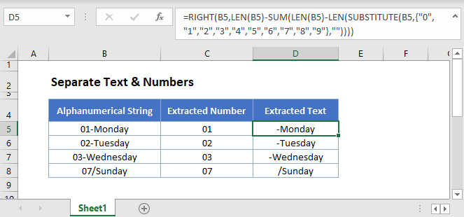
This tutorial will demonstrate you how to separate text and numbers from an alphanumerical string in Excel and Google Sheets.
Separate Number and Text from String
This article will discuss how to split numbers and text if you have alphanumerical data where the first part is text and the last part is numerical (or vis-a-versa).you need only the number part from. For more complex cases see How to Remove Non-Numeric Character article.
Extract Number from the Right
The easiest case of extracting numbers from a string is when the number can be found at the right end of that string. First we locate the starting position of the number with the FIND function and then extract it with the RIGHT function.
=RIGHT(B3,LEN(B3)-MIN(FIND({0,1,2,3,4,5,6,7,8,9},B3&"0123456789"))+1)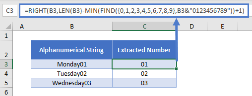
Let’s go through the above formula.
Find First Number
We can use the FIND function to locate the starting position of the number.
=MIN(FIND({0,1,2,3,4,5,6,7,8,9},B3&"0123456789"))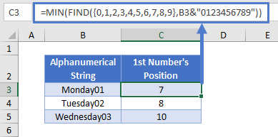
For the find_text argument of the FIND function, we use the array constant {0,1,2,3,4,5,6,7,8,9}, which makes the FIND function perform separate searches for each value in the array constant.
The within_text argument of the FIND function is cell value & “0123456789”. In our example, “Monday010123456789”.
Since the array constant contains 10 numbers, the result will be an array of 10 values. In our example: {7,8,11,12,13,14,15,16,17,18}. Then we simply look for the minimum of number positions within this array and get therefore the place of the first number.
Extract Number Part
Once we have the starting position of the number found at the end of our alphanumerical string, we can use the RIGHT function to extract it.
=RIGHT(B3,LEN(B3)-C3+1)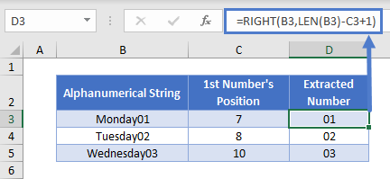
Extract Text Part
With the starting position of the number part we can determine the end of the text part at the same time. We can use the LEFT function to extract it.
=LEFT(B3,C3-1)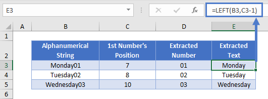
Extract Number from the Left
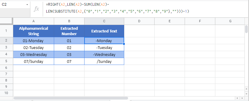
A more complicated case of extracting numbers from a string is when the number can be found at the beginning (i.e., left side) of the string. Obviously, you don’t need to find its starting position, rather the position where it ends. First we find the last number’s position with the help of the SUBSTITUTE function and then extract the number with the LEFT function.
=LEFT(B3,SUM(LEN(B3)-LEN(SUBSTITUTE(B3,{"0","1","2","3","4","5","6","7","8","9"},""))))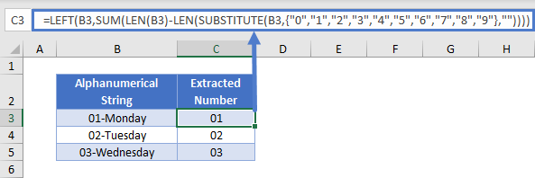
Let’s go through the above formula.
Find Last Number
With the SUBSTITUTE function you can replace every number one by one with an empty string and then sum up how many times you had to do so.
=SUM(LEN(B3)-LEN(SUBSTITUTE(B3,{"0","1","2","3","4","5","6","7","8","9"},"")))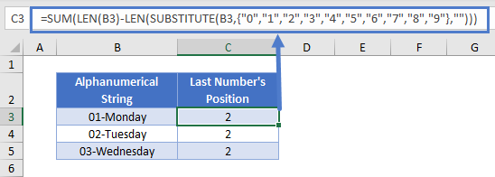
When you substitute each number one by one with an empty string, you get every time a string the length of which is one less the original length. In our case the length of 1-Monday and 0-Monday is both 8. Subtracting this length from the original length (9 in our case), you always get 1. When you sum up these, you get the position of your last number.
Extract Number Part
Once we have the last position of the number found at the beginning of our alphanumerical string, we can use the LEFT function to extract it.
=LEFT(B3,C3)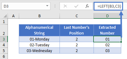
Extract Text Part
Having the last position of the number found at the beginning of our alphanumerical string, we already have the starting position of our text part and can use the RIGHT function to extract it.
=RIGHT(B3,LEN(B3)-C3)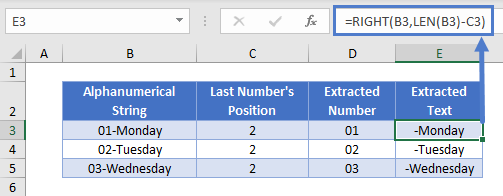
Separate Text & Numbers in Google Sheets
All the examples explained above work the same in Google sheets as they do in Excel.
Many times I get mixed data from field and server for analysis. This data is usually dirty, having column mixed with number ans text. While doing data cleaning before analysis, I separate numbers and text in separate columns. In this article, I’ll tell you how you can do it.
Scenario:
So one our friend on Exceltip.com asked this question in the comments section. “How do I separate numbers coming before a text and in the end of text using excel Formula. For example 125EvenueStreet and LoveYou3000 etc.”
To extracting text, we use RIGHT, LEFT, MID and other text functions. We just need to know the number of texts to extract. And Here we will do the same first.
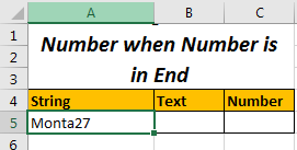
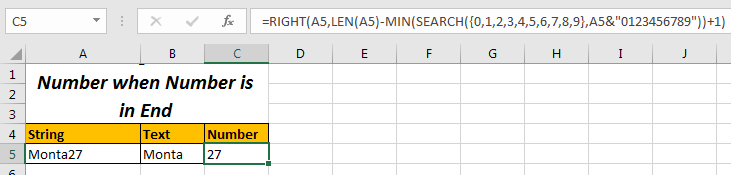
Extract Number and Text from a String when Number is in End of String
For above example I have prepared this sheet. In Cell A2, I have the string. In cell B2, I want the text part and in C2 the Number Part.
So we just need to know the position from where number starts. Then we will use Left and other function. So to get position of first number we use below generic formula:
Generic Formula to Get Position of First Number in String:
=MIN(SEARCH({0,1,2,3,4,5,6,7,8,9},String_Ref&»0123456789″)
This will return the position of first number.
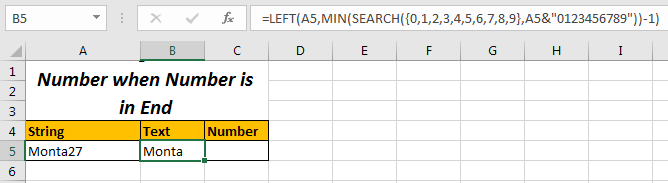
For above example write this formula in any cell.
=MIN(SEARCH({0,1,2,3,4,5,6,7,8,9},A5&»0123456789″))
Extract Text Part
It will return 15 as the first number which is found is at 15th position in Text. I will explain it later.
Now, to get Text, from left we just need to get 15-1 character from string. So we will use
LEFT function to extract text.
Formula to Extract Text from Left
=LEFT(A5,MIN(SEARCH({0,1,2,3,4,5,6,7,8,9},A5&»0123456789″))-1)
Here we just subtracted 1 from what ever number returned by MIN(SEARCH({0,1,2,3,4,5,6,7,8,9},A5&»0123456789″)).
Extract Number Part
Now to get numbers we just need to get number characters from 1st number found. So we calculate the total length of string and subtract the position of first number found and add 1 to it. Simple. Yeah it’s just sound complex, it is simple.
Formula to Extract Numbers from Right
=RIGHT(A5,LEN(A5)-MIN(SEARCH({0,1,2,3,4,5,6,7,8,9},A5&»0123456789″))+1)
Here we just got total length of string using LEN function and then subtracted the position of first found number and then added 1 to it. This gives us total number of numbers. Learn more here about extracting text using LEFT and RIGHT functions of Excel.
So the LEFT and RIGHT function part is simple. The Tricky part is MIN and SEARCH Part that gives us the position of first found number. Let’s understand that.
How It Works
We know how LEFT and RIGHT function work. We will explore the main part of this formula that gets the position of first number found and that is: MIN(SEARCH({0,1,2,3,4,5,6,7,8,9},String&»0123456789″)
The SEARCH function returns the position of a text in string. SEARCH(‘text’,’string’) function takes two argument, first the text you want to search, second the string in which you want to search.
-
- Here in SEARCH, at text position we have an array of numbers from 0 to 9. And at string position we have string which is concatenated with «0123456789» using & operator. Why? I’ll tell you.
- Each element in the array {0,1,2,3,4,5,6,7,8,9} will be searched in given string and will return its position in array form string at same index in array.
- If any value is not found, it will cause an error. Hence all formula will result into an error. To avoid this, we concatenated the numbers «0123456789» in text. So that it always finds each number in string. These numbers are in the end hence will not cause any problem.
- Now The MIN function returns the smallest value from array returned by SEARCH function. This smallest value will be the first number in string. Now using this NUMBER and LEFT and RIGHT function, we can split the text and string parts.
Let’s examin our example. In A5 we have the string that has street name and house number. We need to separate them in different cells.
First let’s see how we got our position of first number in string.
-
- MIN(SEARCH({0,1,2,3,4,5,6,7,8,9},A5&»0123456789″)): this will translate into MIN(SEARCH({0,1,2,3,4,5,6,7,8,9},”Monta270123456789”))
Now, as I explained search will search each number in array {0,1,2,3,4,5,6,7,8,9} in Monta270123456789 and will return its position in an array form. The returned array will be {8,9,6,11,12,13,14,7,16,17}. How?
0 will be searched in string. It is found at 8 position. Hence our first element is 8. Note that our original text is only 7 characters long. Get it. 0 is not a part of Monta27.
Next 1 will be searched in string and it is also not part of original string, and we get it’s position 9.
Next 2 will be searched. Since it is the part of original string, we get its index as 6.
Similarly each element is found at some position.
-
- Now this array is passed to MIN function as MIN({8,9,6,11,12,13,14,7,16,17}). MIN returns the 6 which is position of first number found in original text.
And the story after this is quite simple. We use this number extract text and numbers using LEFT and RIGHT Function.
- Now this array is passed to MIN function as MIN({8,9,6,11,12,13,14,7,16,17}). MIN returns the 6 which is position of first number found in original text.
Extract Number and Text from a String When Number is in Beginning of String
In Above example, Number was in the end of the string. How do we extract number and text when number is in the beginning.
I have prepared a similar table as above. It just has number in the beginning.
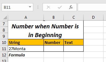
Here we will use a different technique. We will count the length of numbers (which is 2 here) and will extract that number of characters from left of String.
So the method is =LEFT (string, count of numbers)
To Count the Number of characters this is the Formula.
Generic Formula to Count Number of Numbers:
=SUM(LEN(string)-LEN(SUBSTITUTE(string,{«0″,»1″,»2″,»3″,»4″,»5″,»6″,»7″,»8″,»9″},»»))
Here,
-
-
- SUBSTITUTE function will replace each number found with “” (blank). If a number is found ti substituted and new string will be added to array, other wise original string will be added to array. In this way, we will have array of 10 strings.
- Now LEN function will return length of characters in an array of those strings.
- Then, From length of original strings, we will subtract length of each string returned by SUBSTITUTE function. This will again return an array.
- Now SUM will add all these numbers. This is the count of numbers in string.
-
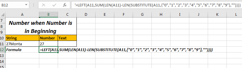
Extract Number Part from String
Now since we know the length of numbers in string, we will substitute this function in LEFT.
Since We have our string an A11 our:
Formula to Extract Numbers from LEFT
=LEFT(A11,SUM(LEN(A11)-LEN(SUBSTITUTE(A11,{«0″,»1″,»2″,»3″,»4″,»5″,»6″,»7″,»8″,»9″},»»))))
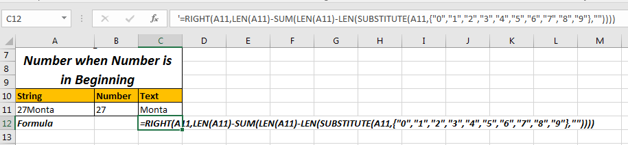
Extract Text Part from String
Since we know number of numbers, we can subtract it from total length of string to get number alphabets in string and then use right function to extract that number of characters from right of the string.
Formula to Extract Text from RIGHT
=RIGHT(A11,LEN(A2)-SUM(LEN(A11)-LEN(SUBSTITUTE(A11,{«0″,»1″,»2″,»3″,»4″,»5″,»6″,»7″,»8″,»9″},»»))))
How it Works
The main part in both formula is SUM(LEN(A11)-LEN(SUBSTITUTE(A11,{«0″,»1″,»2″,»3″,»4″,»5″,»6″,»7″,»8″,»9″},»»))) that calculates the first occurance of a number. Only after finding this, we are able to split text and number using LEFT function. So let’s understand this.
-
-
- SUBSTITUTE(A11,{«0″,»1″,»2″,»3″,»4″,»5″,»6″,»7″,»8″,»9″},»»): This part returns an array of string in A11 after substituting these numbers with nothing/blank (“”). For 27Monta it will return {«27Monta»,»27Monta»,»7Monta»,»27Monta»,»27Monta»,»27Monta»,»27Monta»,»2Monta»,»27Monta»,»27Monta»}.
- LEN(SUBSTITUTE(A11,{«0″,»1″,»2″,»3″,»4″,»5″,»6″,»7″,»8″,»9″},»»)): Now the SUBSTITUTE part is wrapped by LEN function. This return length of texts in array returned by SUBSTITUTE function. In result, we’ll have {7,7,6,7,7,7,7,6,7,7}.
- LEN(A11)-LEN(SUBSTITUTE(A11,{«0″,»1″,»2″,»3″,»4″,»5″,»6″,»7″,»8″,»9″},»»)): Here we are subtracting each number returned by above part from length of actual string. Length of original text is 7. Hence we will have {7-7,7-7,7-6,….}. Finally we will have {0,0,1,0,0,0,0,1,0,0}.
- SUM(LEN(A11)-LEN(SUBSTITUTE(A11,{«0″,»1″,»2″,»3″,»4″,»5″,»6″,»7″,»8″,»9″},»»))): Here we used SUM to sum the array returned by above part of function. This will give 2. Which is number of numbers in string.
-
Now using this we can extract the texts and number and split them in different cells. This method will work with both type text, when number is in beginning and when its in end. You just need to utilize LEFT and RIGHT Function appropriately.
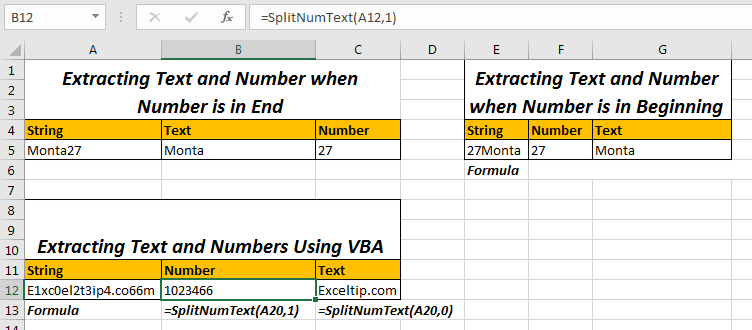
Use SplitNumText function To Split Numbers and Texts from A String
The above to methods are little bit complex and they are not useful when text and numbers are mixed. To split text and numbers use this user defined function.

Syntax:
=SplitNumText(string, op)
String: The String You want to split.
Op: this is boolean. Pass 0 or false to get text part. For number part, pass true or any number greater then 0.
For example, if the string is in A20 then,
Formula for extracting numbers from string is:
=SplitNumText(A20,1)
And
Formula for extracting text from string is:
=SplitNumText(A20,0)
Copy below code in VBA module to make above formula work.
Function SplitNumText(str As String, op As Boolean)
num = ""
   txt = ""
   For i = 1 To Len(str)
       If IsNumeric(Mid(str, i, 1)) Then
            num = num & Mid(str, i, 1)
Else
            txt = txt & Mid(str, i, 1)
     End If
    Next i
If op = True Then
    SplitNumText = num
Else
    SplitNumText = txt
End If
End Function
This code simply checks each character in string, if its a number or not. If it is a number then it is stored in num variable else in txt variable. If user passes true for op then num is returned else txt is returned.
This is the best way to split number and text from a string in my opinion.
You can download the workbook here if you want.
So yeah guys, these are the ways to split text and numbers in different cells. Let me know if you have any doubts or any better solution in the comments section below. Its always fun to interact with guys.
Click the below link to download the working file:
Related Articles:
Extract Text From A String In Excel Using Excel’s LEFT And RIGHT Function
How To Extract Domain Name from EMail in Excel
Split Numbers and Text from String in Excel
Popular Articles:
50 Excel Shortcut’s to Increase Your Productivity
The VLOOKUP Function in Excel
COUNTIF in Excel 2016
How to Use SUMIF Function in Excel
Today, we are going to learn how to separate numbers and text from a cell in Excel. Let’s divide this tutorial into three parts below.


Ok, let’s get started.
Situation 1: Numbers are in front of Text.
This formula allows you quickly get numbers from cell B3.
=-LOOKUP(0,-LEFT(B3,ROW($1:$15)))
ROW($1:$15) indicates the maximum length of the number you want to extract, which can be adjusted according to actual needs. Take an example, if you enter ROW($1:$2), then the cell C3 would only display 12.


Situation 2: Numbers are behind Text
It’s very similar to the last situation. Just enter the formula
=-LOOKUP(0,-RIGHT(B7,ROW($1:$15))) into Cell C7.


Situation 3:Number in the Middle of the text
This situation is more complicated than the above two situations. But its general formula can actually be applied to the above two situations.
=-LOOKUP(1,-RIGHT(LEFT(B11,LOOKUP(10,–MID(B11,ROW($1:$15),1),ROW($1:$15))),ROW($1:$15)))


You can copy the above formulas to use. But if you still want to know the reason or why this code works, we will update the tutorial about the function of LOOKUP. See you next time and Merry Christmas!
Copyright Statement: Regarding all of the posts by this website, any copy or use shall get the written permission or authorization from Myofficetricks.
A very common data cleaning task is to separate numbers from text in 2 different columns. In this post I am going to share with you 3 cases
- Separate numbers from text when the number is at the end of the text
- Separate numbers from text when the number is at the start of the text
- Separate numbers from text when the number is anywhere in the middle of the text (and can also appear multiple times)
And I am going to solve these by using native Excel Formulas and Power Query
Case 1 – Separate numbers from text when the number is at the end of text
Consider this mashup of text and numbers (first column) and from this we need to separate the text and numbers
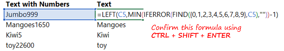
Formula to extract Text
=LEFT(C5,MIN(IFERROR(FIND({0,1,2,3,4,5,6,7,8,9},C5),''))-1)
Formulas to extract Numbers
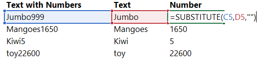
=SUBSTITUTE(C5,D5,'')
- Under the Text column is the formula to extract text. Note that this is an array formula and should be confirmed using CTRL + SHIFT + ENTER
- Once you get the text it is pretty straight forward to get the number. All I do is use a simple the SUBSTITUTE function
Case 2 – Separate numbers from text when the number is at the start of text
Okay, again a similar text-number mashup and this one is a slightly tricky. Let’s parse the numbers and text
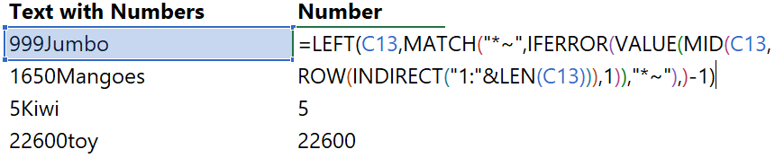
Formula to extract Numbers (Confirm using Ctrl + Shift + Enter)
=LEFT(C13,MATCH('*~',IFERROR(VALUE(MID(C13,ROW(INDIRECT('1:'&LEN(C13))),1)),'*~'),)-1)
Formula to extract Text
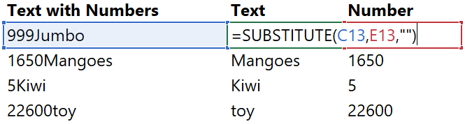
=SUBSTITUTE(C13,E13,'')
- Yeah.. you don’t need to say it, it looks pretty daunting but this nasty buoy works! I am sure this can optimized further but I din’t spend time doing it 🙁
- Although to cool you down the formula for parsing the number is the same old SUBSTITUTE function as above
Case 3 – Separate numbers from text when the number is anywhere in the middle of text
Another tricky situation could be where numbers continuously (or intermittently) appear in the middle of the text string
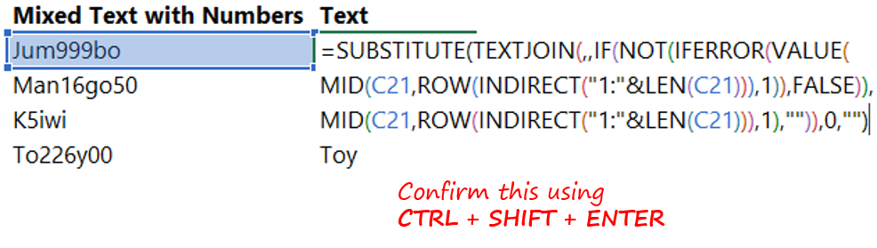
Formula to extract Text
=SUBSTITUTE(TEXTJOIN(,,IF(NOT(IFERROR(VALUE(MID(C21,ROW(INDIRECT('1:'&LEN(C21))),1)),FALSE)),MID(C21,ROW(INDIRECT('1:'&LEN(C21))),1),'')),0,'')
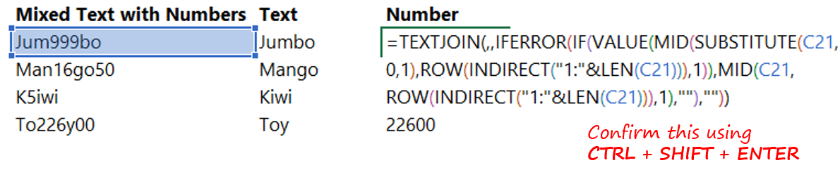
Formula to extract Numbers
=TEXTJOIN(,,IFERROR(IF(VALUE(MID(SUBSTITUTE(C21,0,1),ROW(INDIRECT('1:'&LEN(C21))),1)),MID(C21,ROW(INDIRECT('1:'&LEN(C21))),1),''),''))
- I tackled extracting the text using an array formula again
- But since the numbers have the possibility of appearing intermittently in between so an array formula again for separating the text
Case 4 – Separating Text from Numbers using Power Query
Thankfully power query has a built in option to parse numbers from text or vice versa
Scenario 1 – Numbers in the End of the Text
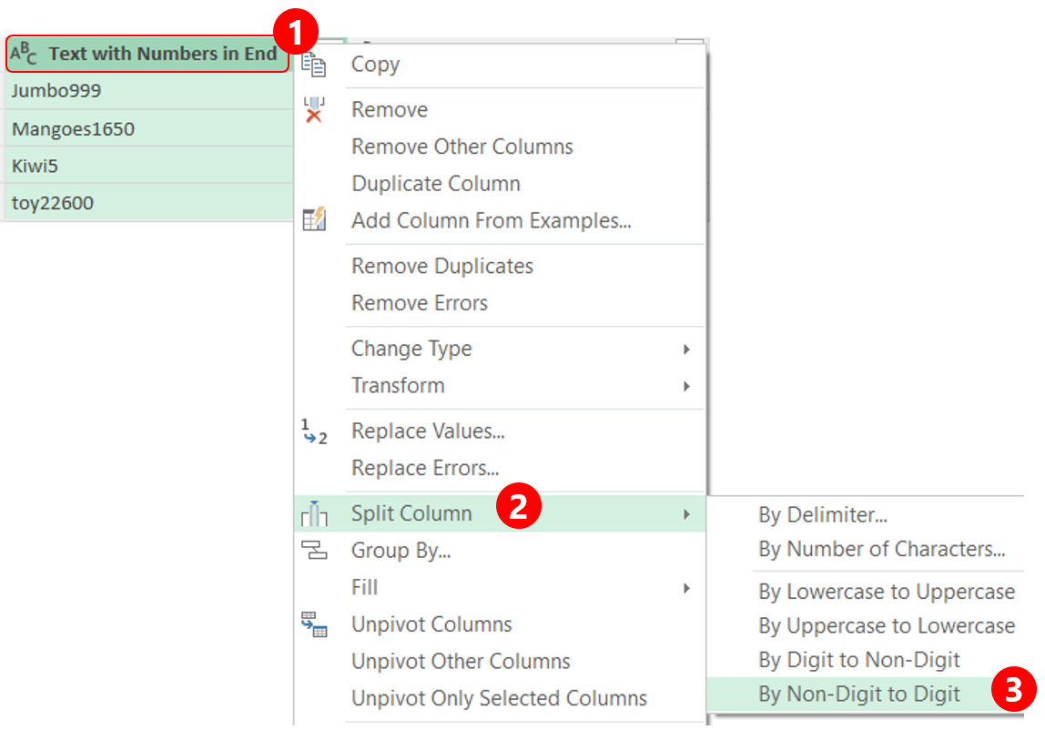
- Just right click on the column header
- In the split menu
- Choose Non-Digit to Digit (i.e. separate at the first digit found)
- And you are done!
Similarly Scenario 2 – Numbers at the Start of the Text
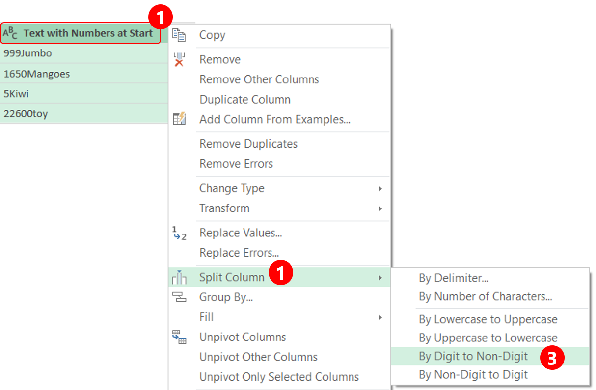
- Just right click on the column header
- In the split menu
- Choose Digit to Non-Digit (i.e. separate at the first text found)
- And you are done!
Feel the need for a video ?
More Excel / Power Pivot / Power Query puzzles..
- Separate Managers and Employee Names
- Unique Dates Challenge – it’ s one of favourite
- Allot the correct shift problem
- Calculate total hours challenge
- Shit timing problem and solution

Chandeep
Welcome to Goodly! My name is Chandeep.
On this blog I actively share my learning on practical use of Excel and Power BI. There is a ton of stuff that I have written in the last few years. I am sure you’ll like browsing around.
Please drop me a comment, in case you are interested in my training / consulting services. Thanks for being around
Chandeep
Only Text
Function Alphas(ByVal strInString As String) As String
Dim lngLen As Long, strOut As String
Dim i As Long, strTmp As String
lngLen = Len(strInString)
strOut = ""
For i = 1 To lngLen
    strTmp = Left$(strInString, 1)
    strInString = Right$(strInString, lngLen - i)
    'The next statement will extract BOTH Lower and Upper case chars
    If (Asc(strTmp) >= 65 And Asc(strTmp) <= 90 Or Asc(strTmp) >= 97 And Asc(strTmp) <= 122) Then
        'to extract just lower case, use the limit 97 - 122
        'to extract just upper case, use the limit 65 - 90
        strOut = strOut & strTmp
    End If
Next i
Alphas = strOut
End Function
Only Numbers
Function Numerics(ByVal strInString As String) As String
Dim lngLen As Long, strOut As String
Dim i As Long, strTmp As String
lngLen = Len(strInString)
strOut = ""
For i = 1 To lngLen
    strTmp = Left$(strInString, 1)
    strInString = Right$(strInString, lngLen - i)
    If (Asc(strTmp) >= 48 And Asc(strTmp) <= 57) Then
        strOut = strOut & strTmp
    End If
Next i
Numerics = strOut
End Function
Only Number & Text
Function Alphanumerics(ByVal strInString As String) As String
Dim lngLen As Long, strOut As String
Dim i As Long, strTmp As String
lngLen = Len(strInString)
strOut = ""
For i = 1 To lngLen
    strTmp = Left$(strInString, 1)
    strInString = Right$(strInString, lngLen - i)
    'The next statement will extract BOTH Lower and Upper case chars
    If (Asc(strTmp) >= 65 And Asc(strTmp) <= 90 Or Asc(strTmp) >= 97 And Asc(strTmp) <= 122 or Asc(strTmp) >= 48 And Asc(strTmp) <= 57) Then
        'to extract just lower case, use the limit 97 - 122
        'to extract just upper case, use the limit 65 - 90
        strOut = strOut & strTmp
    End If
Next i
Alphanumerics = strOut
End Function
This can use in excel too but this is modified by me for Access use