
Excel for Microsoft 365 Excel 2021 Excel 2019 Excel 2016 Excel 2013 More…Less
You might want to split a cell into two smaller cells within a single column. Unfortunately, you can’t do this in Excel. Instead, create a new column next to the column that has the cell you want to split and then split the cell. You can also split the contents of a cell into multiple adjacent cells.
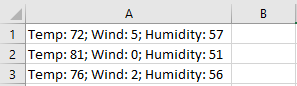
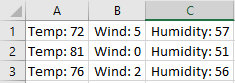
See the following screenshots for an example:
Split the content from one cell into two or more cells
-
Select the cell or cells whose contents you want to split.
Important: When you split the contents, they will overwrite the contents in the next cell to the right, so make sure to have empty space there.
-
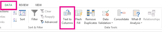
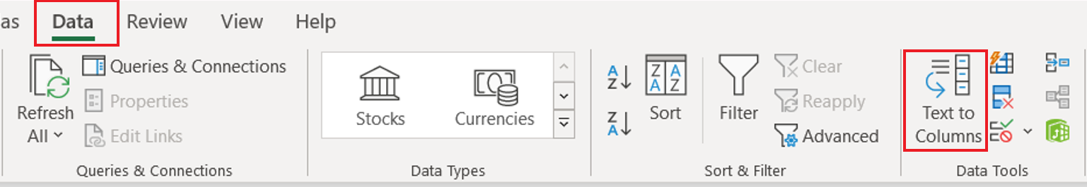
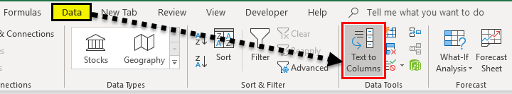
On the Data tab, in the Data Tools group, click Text to Columns. The Convert Text to Columns Wizard opens.

-
Choose Delimited if it is not already selected, and then click Next.
-
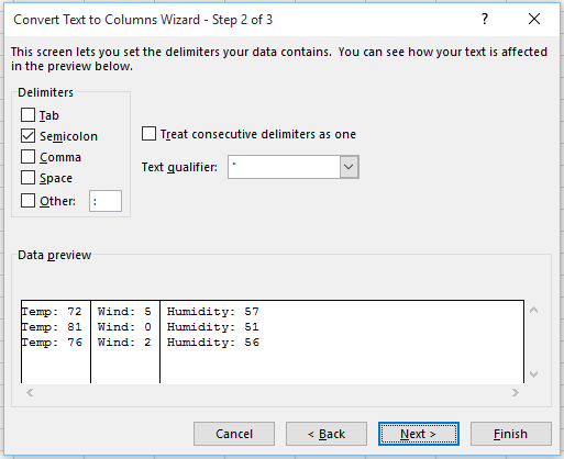
Select the delimiter or delimiters to define the places where you want to split the cell content. The Data preview section shows you what your content would look like. Click Next.
-
In the Column data format area, select the data format for the new columns. By default, the columns have the same data format as the original cell. Click Finish.
See Also
Merge and unmerge cells
Merging and splitting cells or data
Need more help?
Want more options?
Explore subscription benefits, browse training courses, learn how to secure your device, and more.
Communities help you ask and answer questions, give feedback, and hear from experts with rich knowledge.
Sometimes you may have the text and numeric data in the same cell, and you may have a need to separate the text portion and the number portion in different cells.
While there is no inbuilt method to do this specifically, there are some Excel features and formulas you can use to get this done.
In this tutorial, I will show you 4 simple and easy ways to separate text and numbers in Excel.
Let’s get to it!
Separate Text and Numbers Using Flash Fill
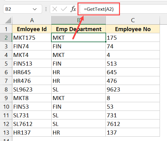
Below I have the employee data in column A, where the first few alphabets indicate the department of the employee and the numbers after it indicates the employee number.

From this data, I want to separate the text part and the number part and get these into two separate columns (columns B and C).
The first method that I want to show you to separate text and numbers in Excel is by using Flash Fill.
Flash Fill (introduced in Excel 2013) works by identifying patterns based on user input.
So if I manually enter the expected result in column B, Flash Fill will try and decipher the pattern and give me the result for all the cells in that column.
Below are the steps to separate the text part from the cell and get it in column B:
- Select cell B2
- Manually enter the expected result in cell B2, which would be MKT

- With cell B2 selected, place the cursor at the bottom right part of the selection. You’ll notice that the cursor changes into a plus icon (this is called Fill Handle)

- Hold the left mouse/trackpad key and drag the Fill Handle to fill the cells. Don’t worry if the cells are filled with the same text
- Click on the Auto Fill Options icon and then select the ‘Flash Fill’ option

The above steps would extract the text part from the cells in column A and give you the result in column B.

Note that in some cases, Flash Fill may not be able to identify the right pattern. In such cases, it would be best to enter the expected result in two or three cells, use the Fill Handle to fill the entire column, and then use Flash Fill on this data.
You can follow the same process to extract the numbers in column C. All you need to do is enter the expected result in cell C2 (step 2 in the process laid out above)
Note that the result you get from Flash Fill is static and would not update in case you change the original data in column A. If you want the result to be dynamic, you can use the formula method covered next.
Separate Text and Numbers Using Formula
Below I have the employee data in column A and I want to use a formula to extract only the text part and put it in column B and extract the number part and put it in column C.
Since the data is not consistent (i.e., the alphabets in the department code and the numbers in the employee number are not of the consistent length), I cannot use the LEFT or RIGHT function to extract only the text portion or only the number portion.
Below is the formula that will extract only the text portion from the left:
=LEFT(A2,MIN(IFERROR(FIND({0,1,2,3,4,5,6,7,8,9},A2),""))-1)

And below is the formula that will extract all the numbers from the right:
=MID(A2,MIN(IFERROR(FIND({0,1,2,3,4,5,6,7,8,9},A2),"")),100)

How does this formula work?
Let me first explain the formula that we use to separate the text part on the left.
=LEFT(A2,MIN(IFERROR(FIND({0,1,2,3,4,5,6,7,8,9},A2),””))-1)
The FIND part in the formula finds the position of digits 0 to 9 in cell A2. In case it finds that digit in cell A2, it returns the position of that digit, and in case it is not able to find that digit, then it returns the value error (#VALUE!)
For cell A2, it gives a result as shown below:
{#VALUE!,4,#VALUE!,#VALUE!,#VALUE!,6,#VALUE!,5,#VALUE!,#VALUE!}
- For 0, it returns #VALUE! as it cannot find this digit in cell A2
- For 1, it returns 4 as that is the position of the first occurrence of 1 in cell A2
- and so on…
This FIND formula is then wrapped inside the IFERROR function, which removes all the value errors but leaves the numbers.
The result of it looks like as shown below:
{“”,4,””,””,””,6,””,5,””,””}
The MIN function then goes through the above result and gives us the minimum value from the results. Since each number in the array represents the position of that corresponding number, the minimum value tells us where the numerical value starts in the cell.
Now that we know where the numerical values start, I have used the LEFT function to extract everything before this position (which would be all the text in the cell).
Similarly, you can use the same formula with a minor tweak to extract all the numbers after the text. To extract the numbers, where we know the starting position of the first digit, use the MID function to extract everything starting from that position.
And what if the situation is reversed – where we have the numbers first and the text later and we want to separate the numbers and text?
You can still use the same logic with one minor change – instead of finding the minimum value that gives us the position of the 1st digit in the cell, you need to use the MAX function To find the position of the last digit in this cell. Once you have it, you can again use the LEFT function or the MID function to separate the numbers and text.
Separate Text and Numbers Using VBA (Custom Function)
While you can use the formulas shown above to separate the text and numbers in a cell and extract these into different cells – if this is something you need to do quite often, you also have the option to create your own custom function using VBA.
The benefit of creating your own function would be that it would be a lot easier to use (with just one function that takes only one argument).
You can also save this custom function VBA code into the Personal Macro Workbook so that it would be available in all your Excel workbooks.
Below the VBA code that could create a function ‘GetNumber’ that would take the cell reference as the input argument, extract all the numbers in the cell, and give it as the result.
'Code created by Sumit Bansal from https://trumpexcel.com
'This code will create a function that can separate numbers from a cell
Function GetNumber(CellRef As String)
Dim StringLength As Integer
StringLength = Len(CellRef)
For i = 1 To StringLength
If IsNumeric(Mid(CellRef, i, 1)) Then Result = Result & Mid(CellRef, i, 1)
Next i
GetNumber = Result
End Function
And below the VBA code that would create another function ‘GetText’ that would take the cell reference as the input argument and give you all the text from that cell
'Code created by Sumit Bansal from https://trumpexcel.com
''This code will create a function that can separate text from a cell
Function GetText(CellRef As String)
Dim StringLength As Integer
StringLength = Len(CellRef)
For i = 1 To StringLength
If Not (IsNumeric(Mid(CellRef, i, 1))) Then Result = Result & Mid(CellRef, i, 1)
Next i
GetText = Result
End Function
Below are the steps to add this code to your excel workbook so that this function becomes available for you to use in the worksheet:
- Click the Developer tab in the ribbon
- Click on the Visual Basic icon

- In the Visual Basic editor that opens up, you would see the Project Explorer on the left. This would have the workbook and the worksheet names of your current Excel workbook. If you don’t see this, click on the View option in the menu and then click on Project Explorer

- Select any of the sheet names (or any object) for the workbook in which you want to add this function
- Click on the Insert option in the top toolbar and then click on Module. This will insert a new module for that workbook

- Double click on the module icon in ‘Project Explorer’. This will open the module code window.

- Copy and paste the above custom function code into the module code window

- Close the VB Editor
With the above steps, we have added the custom function code to the Excel workbook.
Now you can use the functions =GETNUMBER or =GETTEXT just like any other worksheet function.
Note – Once you have the macro code in the module code window, you need to save the file as a Macro Enabled file (with the .xlsm extension instead of the .xlsx extension)
If you often have a need to separate text numbers from cells in Excel, it would be more efficient if you copy these VBA codes for creating these custom functions, and save these in your Personal Macro Workbook.
You can learn how to create and use Personal Macro Workbook in this tutorial I created earlier.
Once you have these functions in the Personal Macro Workbook, you would be able to use these on any Excel workbook on your system.
One important thing to remember when using functions that are stored in Personal Macro Workbook – you need to prefix the function name with =PERSONAL.XLSB!. For example, if I want to use the function GETNUMBER in a workbook in Excel, and I have saved the code for it in the postal macro workbook, I will have to use =PERSONAL.XLSB!GETNUMBER(A2)
Separate Text and Numbers Using Power Query
Power Query is slowly becoming my favorite feature in Excel.
If you’re already using Power Query as a part of your workflow, and you have a data set where you want to separate the text and numbers into separate columns, Power Query will do it in a few clicks.
When you have your data in Excel and you want to use Power Query to transform that data, one prerequisite is to convert that data into an Excel Table (or a named range).
Below I have an Excel Table that contains the data where I want to separate the text and number portions into separate columns.

Here are the steps to do this:
- Select any cell in the Excel Table
- Click the Data tab in the ribbon

- In the Get and Transform group, click on the ‘From Table/Range’

- In the Power Query editor that opens up, select the column from which you want to separate the numbers and text
- Click the Transform tab in the Power Query ribbon

- Click on the Split Column option

- Click on ‘By Non Digit to Digit’ option.

- You’ll see that the column has been split into two columns where one has only the text and the other only has the numbers

- [Optional] Change the column names if you want
- Click the Home tab and then click on Close and Load. This will insert a new sheet and give us the output as an Excel Table.

The above steps would take the data from the Excel Table we originally had, use Power Query to split the column and separate the text and the number parts into two separate columns, and then give us back the output in a new sheet in the same workbook.

Note that we used the option ‘By Non-Digit to Digit’ option in step 7, which means that every time there is a change from a non-digit character to a digit, a split would be made. If you have a dataset where the numbers are first followed by text, you can use the ‘By Digit to Non-Digit’ option
Now let me tell you the best part about this method. Your original Excel Table (which is the data source) is connected to the output Excel Table.
So if you make any changes in your original data, you don’t need to repeat the entire process. You can simply go to any cell in the output Excel Table, right click and then click on Refresh.
Power query would run in the back end, check the entire original data source, do all the transformations that we did in the steps above, and update your output result data.
This is where Power Query really shines. If there is a set of transformations that you often need to do on a data set, you can use Power Query to do that transformation once and set the process. Excel would create a connection between the original data source and the resulting output data and remember all the steps you had taken to transform this data.
Now, if you get a new data set you can simply put it in the place of your original data and refresh the query, and you will get the result in a few seconds. Alternatively, you can simply change the source in Power Query from the existing Excel table to some other Excel Table (in same or different workbook).
So these are four simple ways you can use to separate numbers and text in Excel. if this is a once-in-a-while activity, you’re better off using Flash Fill or the formula method.
And in case this is something you need to do quite often, then I would suggest you consider the VBA method where we created a custom function or the Power Query method.
I hope you found this Excel tutorial useful.
Other Excel tutorials you may also like:
- Separate First and Last Name in Excel (Split Names Using Formulas)
- How to Convert Numbers to Text in Excel
- Convert Text to Numbers in Excel – A Step By Step Tutorial
- How to Compare Text in Excel
- How to Quickly Combine Cells in Excel
- How to Combine First and Last Name in Excel
- How to Extract the First Word from a Text String in Excel (3 Easy Ways)
- Extract Numbers from a String in Excel (Using Formulas or VBA)
- How to Extract a Substring in Excel (Using TEXT Formulas)
Note: This guide on how to split cells in Excel is suitable for all versions of Excel.
In your Excel journey, you will come across situations where you have to work with imported data. In these cases, it is very common to find cells of data that are not in the desired format.
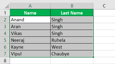
For example, I have an Excel sheet, where a column of cells displays both the first and last names of customers together. But, I need to split the cells into two separate columns for the first and last names.
Related:
How To Find Duplicates In Excel? The Best Guide
Excel Goal Seek—the Easiest Guide (3 Examples)
Create A Pivot Table In Excel—the Easiest Guide
In other words, how to split cells across multiple columns?
In this guide, I’ll explain three easy ways to split cells in Excel with ample illustrations. You can watch this short video to easily learn how to split cells in Excel.
Please find below the sample Excel sheet to download and follow along with me.

- How to Split Cells in Excel Using Text to Column?
- How to Split Cells in Excel Using Text Functions?
- How to Split Cells Using Flash Fill (Auto Fill)?
- FAQs
How to Split Cells in Excel Using Text to Column?
One of the easiest ways to split cells is to use the text to column feature. To do this do the following:
- Select the column of cells you want to split. You can also select a specific range in a column.

- Locate and click on the Text to Columns button under the Data tab. It can be found in the Data Tools section.
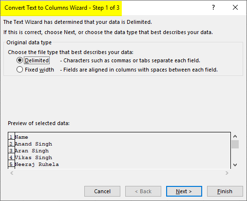
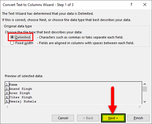
- In the Convert Text to Columns Wizard, select the Delimited option as the data type.

Click Next.
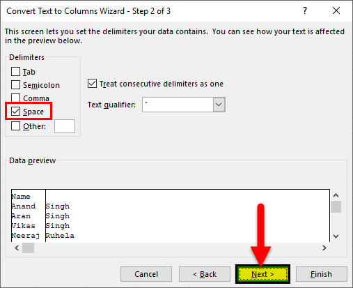
- In the next window, select the Delimiters for splitting your cells. A delimiter is the character based on which the split should happen. In this case, the names have a space between them. Hence, the delimiter here is Space.
Also Read:
How To Use Excel Countifs: The Best Guide
Excel Conditional Formatting -the Best Guide (Bonus Video)
The Best Excel Project Management Template In 2021
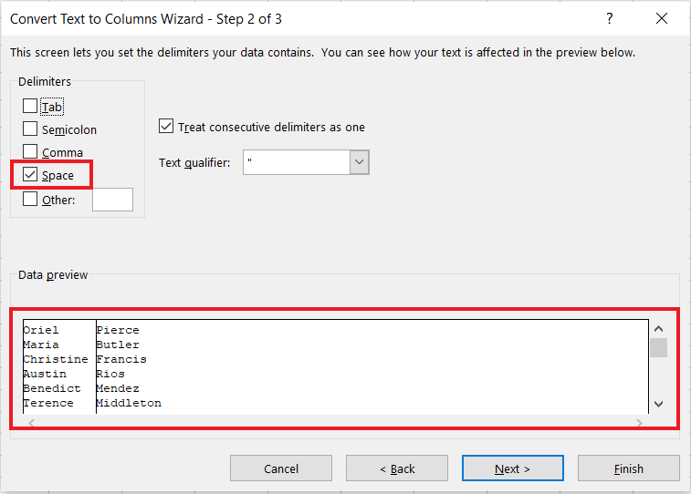
Note that, any delimiter can be used if the data has it. If you are confused about which one to select, use trial and error to see how your split data appears in the Data preview window.
Click on Next.
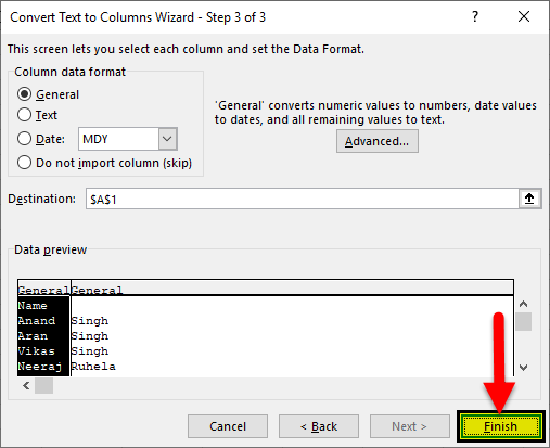
- Now, choose your Data Type and Enter your Destination cell. In this example the destination cell is B2. keep in mind to leave sufficient space, especially if there are multiple delimiters in your data.

Click on Finish.
Congratulations, your cells have split into multiple cells. Keep in mind that this is not a dynamic feature. It means that any later change in the original names or data will not reflect in the result column.

How to Split Cells in Excel Using Text Functions?
Sometimes, you need a more robust solution to splitting cells. For example, the data may not contain a standard delimiter for you to choose. Or you may need to make the splitting process dynamic.
For such cases, use the Text functions to split the cells.
There are many text functions in Excel, but we don’t need all of them here. A few important ones are:
1. LEN – Returns the length of a string
2. RIGHT – Extract a specified number of characters from a String’s right end.
3. LEFT – Extract a specified number of characters from a String’s left end.
4. FIND – Look for a string inside another string.
5. SEARCH – Return the positions of a string inside another string
6. MID – Extract a specified number of characters from a String’s centre.
There is no one standard way to do this. You can use any combination of the above text functions to achieve your split.
Now, I’ll show you how to implement this using simple examples. Do the following:
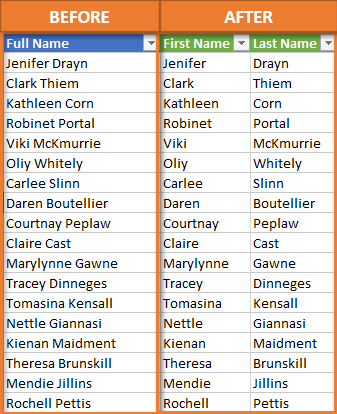
- Determine the type of split you want in the data. I am using the same example, where the first names and last names are separated by a space.
- Now, to extract the first name, use a combination of SEARCH and LEFT functions.
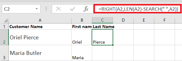
Enter the formula =LEFT(A2,SEARCH(” “,A2)-1) in cell B2.
Here, the SEARCH looks for any space in the customer name and returns its position in the string. Then, the LEFT function extracts the part of the string from the left side, up to the position returned by the SEARCH function.

- Drag the formula to all the cells below.
You have successfully extracted the first names.
- Now, repeat the same process to extract the last names, except here, use the RIGHT function to extract from the end of the string.
Enter the formula =RIGHT(A2,LEN(A2)-SEARCH(” “,A2)) in cell C2.
Here, the SEARCH looks for any space in the customer name and returns its position in the string. Then, the RIGHT function extracts the part of the string from the right side, up to the position, returned by the SEARCH function.
Drag the formula to all the cells below.
- Congratulations, you have successfully split the first and last names.
- The most important thing to note here is that the split is dynamic. That is, when you change the source data, the results also change automatically.

How to Split Cells Using Flash Fill (Auto Fill)?
Sometimes, you may want to split cells without using any formula or wizard menus.
To do this, use the Flash Fill feature to split cells instantly.
Follow these simple steps to accomplish this:
1. Type in the neighbouring cell, in the next column, an example of the split cell.
2. Drag the fill handle till the end of the data range.
3. Click on the AutoFill Options button at the end of the range and select Flash Fill

Now, Excel will recognize the pattern and will fill the remaining cells for you. Repeat the same process for the last names. You have successfully split the cells.
Suggested Reads:
Create An Excel Dashboard In 5 Minutes – The Best Guide
Dynamic Dropdown Lists In Excel – Top Data Validation Guide
Predict Future Values Using Excel Forecast Sheet – The Best Guide
FAQs
How to split cells in Excel to extract data?
You can split cells in Excel using these three methods.
1. Use the Text to Column feature to split cells with delimiter.
2. Use Text functions to split cells if you need a dynamic split.
3. Use Flash Fill in the Auto Fill feature to automatically split strings in cells.
Is there a split function in Excel?
Yes, there is a SPLIT function in Excel, which uses a delimiter to split strings into smaller sub strings.
Let’s Wrap Up
In this guide, I have explained how to split cells in Excel in a step-by-step manner. I have covered all three important methods to split cells with detailed examples. If you have any doubts regarding splitting cells or any other Excel feature, please let us know in the comments below.
If you need more high-quality Excel guides, please check out our free Excel resources centre.
Simon Sez IT has been teaching Excel for over ten years. For a low, monthly fee you can get access to 100+ IT training courses. Click here for advance Excel courses with in-depth training modules.

Adam Lacey

Adam Lacey is an Excel enthusiast and online learning expert. He combines these two passions at Simon Sez IT where he wears a number of different hats.When Adam isn’t fretting about site traffic or Pivot Tables, you’ll find him on the tennis court or in the kitchen cooking up a storm.
When data is imported into Excel it can be in many formats depending on the source application that has provided it.
For example, it could contain names and addresses of customers or employees, but this all ends up as a continuous text string in one column of the worksheet, instead of being separated out into individual columns e.g. name, street, city.
You can split the data by using a common delimiter character. A delimiter character is usually a comma, tab, space, or semi-colon. This character separates each chunk of data within the text string.
A big advantage of using a delimiter character is that it does not rely on fixed widths within the text. The delimiter indicates exactly where to split the text.
You may need to split the data because you may want to sort the data using a certain part of the address or to be able to filter on a particular component. If the data is used in a pivot table, you may need to have the name and address as different fields within it.
This article shows you eight ways to split the text into the component parts required by using a delimiter character to indicate the split points.
Sample Data
The above sample data will be used in all the following examples. Download the example file to get the sample data plus the various solutions for extracting data based on delimiters.
Excel Functions to Split Text
There are several Excel functions that can be used to split and manipulate text within a cell.
LEFT Function
The LEFT function returns the number of characters from the left of the text.
Syntax
= LEFT ( Text, [Number] )- Text – This is the text string that you wish to extract from. It can also be a valid cell reference within a workbook.
- Number [Optional] – This is the number of characters that you wish to extract from the text string. The value must be greater than or equal to zero. If the value is greater than the length of the text string, then all characters will be returned. If the value is omitted, then the value is assumed to be one.
RIGHT Function
The RIGHT function returns the number of characters from the right of the text.
Syntax
= RIGHT ( Text, [Number] )The parameters work in the same way as for the LEFT function described above.
FIND Function
The FIND function returns the position of specified text within a text string. This can be used for locating a delimiter character. Note that the search is case-sensitive.
Syntax
= FIND (SubText, Text, [Start])- SubText – This is a text string that you want to search for.
- Text – This is the text string which is to be searched.
- Start [Optional] – The starting position for the search.
LEN Function
The LEN function will give the length by number of characters of a text string.
Syntax
= LEN ( Text )- Text – This is the text string of which you want to determine the character count.
Extracting Data with the LEFT, RIGHT, FIND and LEN Functions
Using the first row (B3) of the sample data, these functions can be combined to split a text string into sections using a delimiter character.
= FIND ( ",", B3 )You use the FIND function to get the position of the first delimiter character. This will return the value 18.
= LEFT ( B3, FIND( ",", B3 ) - 1 )You can then use the LEFT function to extract the first component of the text string.
Note that FIND gets the position of the first delimiter, but you need to subtract 1 from it so as to not include the delimiter character.
This will return Tabbie O’Hallagan.
= RIGHT ( B3, LEN ( B3 ) - FIND ( ",", B3 ) )It is more complicated to get the next components of the text string. You need to remove the first component from the text by using the above formula.
This formula takes the length of the original text, finds the first delimiter position, which then calculates how many characters are left in the text string after that delimiter.
The RIGHT function then truncates off all the characters up to and including that first delimiter so that the text string gets shorter and shorter as each delimiter character is found.
This will return 056 Dennis Park, Greda, Croatia, 44273
You can now use FIND to locate the next delimiter and the LEFT function to extract the next component, using the same methodology as above.
Repeat for all delimiters, and this will split the text string into component parts.
FILTERXML Function as a Dynamic Array
If you’re using Excel for Microsoft 365, then you can use the FILTERXML function to split text with output as a dynamic array.
You can split a text string by turning it into an XML string by changing the delimiter characters to XML tags. This way you can use the FILTERXML function to extract data.
XML tags are user defined, but in this example, s will represent a sub-node and t will represent the main node.
= "<t><s>" & SUBSTITUTE ( B2, ",", "</s><s>" ) & "</s></t>"Use the above formula to insert the XML tags into your text string.
<t><s>Name</s><s>Street</s><s>City</s><s>Country</s><s>Post Code</s></t>This will return the above formula in the example.
Note that each of the nodes defined is followed by a closing node with a backslash. These XML tags define the start and finish of each section of the text, and effectively act in the same way as delimiters.
=TRANSPOSE(
    FILTERXML(
        "<t><s>" &
        SUBSTITUTE(
            B3,
            ",",
            "</s><s>"
        ) & "</s></t>",
        "//s"
    )
)
The above formula will insert the XML tags into the original string and then use these to split out the items into an array.
As seen above, the array will spill each item into a separate cell. Using the TRANSPOSE function causes the array to spill horizontally instead of vertically.
FILTERXML Function to Split Text
If your version of Excel doesn’t have dynamic arrays, then you can still use the FILTERXML function to extract individual items.
= FILTERXML (
    "<t><s>" &
    SUBSTITUTE (
        B3,
        ",",
        "</s><s>"
    ) & "</s></t>",
    "//s"
)
You can now break the string into sections using the above FILTERXML formula.
This will return the first section Tabbie O’Hallagan.
= FILTERXML (
    "<t><s>" &
    SUBSTITUTE (
        B3,
        ",",
        "</s><s>"
    ) & "</s></t>",
    "//s[2]"
)
To return the next section, use the above formula.
This will return the second section of the text string 056 Dennis Park.
You can use this same pattern to return any part of the sample text, just change the [2] found in the formula accordingly.
Flash Fill to Split Text
Flash Fill allows you to put in an example of how you want your data split.
You can check out this guide on using flash fill to clean your data for more details.
You then select the first cell of where you want your data to split and click on Flash Fill. Excel will populate the remaining rows from your example.
Using the sample data, enter Name into cell C2, then Tabbie O’Hallagan into cell C3.
Flash fill should automatically fill in the remaining data names from the sample data. If it doesn’t, you can select cell C4, and click on the Flash Fill icon in the Data Tools group of the Data tab of the Excel ribbon.
Similarly, you can add Street into cell D2, City into cell E2, Country into cell F2, and Post Code into cell G2.
Select the subsequent cells (D2 to G2) individually, and click on the Flash Fill icon. The rest of the text components will be populated into these columns.
Text to Columns Command to Split Text
This Excel functionality can be used to split text in a cell into sections based on a delimiter character.
- Select the entire sample data range (B2:B12).
- Click on the Data tab in the Excel ribbon.
- Click on the Text to Columns icon in the Data Tools group of the Excel ribbon and a wizard will appear to help you set up how the text will be split.
- Select Delimited on the option buttons.
- Press the Next button.
- Select Comma as the delimiter, and uncheck any other delimiters.
- Press the Next button.
- The Data Preview window will display how your data will be split. Choose a location to place the output.
- Click on Finish button.
Your data will now be displayed in columns on your worksheet.
Convert the Data into a CSV File
This will only work with commas as delimiters, since a CSV (comma separated value) file depends on commas to separate the values.
Open Notepad and copy and paste the sample data into it. You can open Notepad by typing Notepad into the search box at the left of the Windows task bar or locate it in the application list.
Once you have copied the data into Notepad, save it off by using File ➜ Save As from the menu. Enter a filename with a .csv suffix e.g. Split Data.csv.
You can then open this file in Excel. Select the csv file in the browser file type drop down and click OK. Your data will automatically appear with each component in separate columns.
VBA to Split Text
VBA is the programming language that sits behind Excel and allows you to write your own code to manipulate data, or to even create your own functions.
To access the Visual Basic Editor (VBE), you use Alt + F11.
Sub SplitText()

Dim MyArray() As String, Count As Long, i As Variant

For n = 2 To 12
	MyArray = Split(Cells(n, 2), ",")
	Count = 3
	For Each i In MyArray
		Cells(n, Count) = i
		Count = Count + 1
	Next i
Next n

End Sub
Click on Insert in the menu bar, and click on Module. A new pane will appear for the module. Paste in the above code.
This code creates a single dimensional array called MyArray. It then iterates through the sample data (rows 2 to 12) and uses the VBA Split function to populate MyArray.
The split function uses a comma delimiter, so that each section of the text becomes an element of the array.
A counter variable is set to 3 which represents column C, which will be the first column for the split data to be displayed.
The code then iterates through each element in the array and populates each cell with the element. Cell references are based on n for the row, and Count for the column.
The variable Count is incremented in each loop so that the data fills across the row, and then downwards.
Power Query to Split Text
Power Query in Excel allows a column to be manipulated into sections using a delimiter character.
Related posts:
- Introduction to power query
- Power query tips and tricks
- Introduction to power query M code
The first thing to do is to define your data source, which is the sample data that you entered into you Excel worksheet.
Click on the Data tab in the Excel ribbon, and then click on Get Data in the Get & Transform Data group of the ribbon.
Click on From File in the first drop down, and then click on From Workbook in the second drop down.
This will display a file browser. Locate your sample data file (the file that you have open) and click on OK.
A navigation pop-up will be displayed showing all the worksheets within your workbook. Click on the worksheet which has the sample data and this will show a preview of the data.
Expand the tree of data in the left-hand pane to show the preview of the existing data.
Click on Transform Data and this will display the Power Query Editor.
Make sure that the single column with the data in it is highlighted. Click on the Split Column icon in the Transform group of the ribbon. Click on By Delimiter in the drop down that appears.
This will display a pop-up window which allows you to select your delimiter. The default is a comma.
Click OK and the data will be transformed into separate columns.
Click on Close and Load in the Close group of the ribbon, and a new worksheet will be added to your workbook with a table of the data in the new format.
Power Pivot Calculated Column to Split Text
You can use Power Pivot to split the text by using calculated columns.
Click on the Power Pivot tab in the Excel ribbon and then click on the Add to Data Model icon in the Tables group.
Your data will be automatically detected and a pop-up will show the location. If this is not the correct location, then it can be re-set here.
Leave the My table has headers check box un-ticked in the pop-up, as we want to split the header as well.
Click on OK and a preview screen will be displayed.
Right-click on the header for your data column (Column1) and click on Insert Column in the pop-up menu. This will insert a calculated column where a formula can be entered.
= LEFT ( [Column1], FIND ( ",", [Column1] ) - 1 )In the formula bar, insert the above formula.
This works in a similar way to the functions described in method 1 of this article.
This formula will provide the Name component within the text string.
Insert another calculated column using the same methodology as the first calculated column.
= LEFT (
    RIGHT ( [Column1], LEN ( [column1] ) - LEN ( [Calculated Column 1] ) - 1 ),
    FIND (
        ",",
        RIGHT ( [Column1], LEN ( [column1] ) - LEN ( [Calculated Column 1] ) - 1 )
    ) - 1
)
Insert the above formula into the formula bar.
This is a complicated formula, and you may wish to break it into sections using several calculated columns.
This will provide the Street component in the text string.
You can continue modifying the formula to create calculated columns for all the other components of the text string.
The problem with a pivot table is that it needs a numeric value as well as text values. As the sample data is text only, a numeric value needs to be added.
Click on the first cell in the Add Column column and enter the formula =1 in the formula bar.
This will add the value of 1 all the way down that column. Click on the Pivot Table icon in the Home tab of the ribbon.
Click on Pivot Table in the pop-up menu. Specify the location of your pivot table in the first pop-up window and click OK. If the Pivot Table Fields pane does not automatically display, right click on the pivot table skeleton and select Show Field List.
Click on the Calculated Columns in the Field List and place these in the Rows window.
our pivot table will now show the individual components of the text string.
Conclusions
Dealing with comma or other delimiter separated data can be a big pain if you don’t know how to extract each item into its own cell.
Thankfully, Excel has quite a few options that will help with this common task.
Which one do you prefer to use?
About the Author
John is a Microsoft MVP and qualified actuary with over 15 years of experience. He has worked in a variety of industries, including insurance, ad tech, and most recently Power Platform consulting. He is a keen problem solver and has a passion for using technology to make businesses more efficient.
Bottom Line: Learn how to use formulas and functions in Excel to split full names into columns of first and last names.
Skill Level: Intermediate
Watch the Tutorial
Download the Excel Files
You can download both the before and after files below. The before file is so you can follow along, and the after file includes all of the formulas already written.
Splitting Text Into Separate Columns
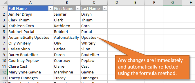
We’ve been talking about various ways to take the text that is in one column and divide it into two. Specifically, we’ve been looking at the common example of taking a Full Name column and splitting it into First Name and Last Name.
The first solution we looked at used Power Query and you can view that tutorial here: How to Split Cells and Text in Excel with Power Query. Then we explored how to use the Text to Columns feature that’s built into Excel: Split Cells with Text to Columns in Excel. Today, I want to show you how to accomplish the same thing with formulas.
Using 4 Functions to Build our Formulas
To split our Full Name column into First and Last using formulas, we need to use four different functions. We’ll be using SEARCH and LEFT to pull out the first name. Then we’ll use LEN and RIGHT to pull out the last name.
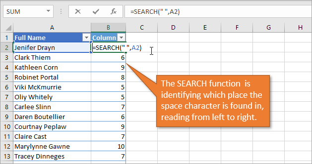
The SEARCH Function
They key to breaking up the first names from the last names is for Excel to identify what all of the full names have in common. That common factor is the space character that separates the two names. To help our formula identify everything to the left of that space character as the first name, we need to use the SEARCH function.
The SEARCH function returns the number of the character at which a specific character or text string is found, reading left to right. In other words, what number is the space character in the line of characters that make up a full name? In my name, Jon Acampora, the space character is the 4th character (after J, o, and n), so the SEARCH function returns the number 4.
There are three arguments for SEARCH.
- The first argument for the SEARCH function is find_text. The text we want to find in our entries is the space character. So, for find_text, we enter ” “, being sure to include the quotation marks.
- The second argument is within_text. This is the text we are searching in for the space character. That would be the cell that has the full name. In our example, the first cell that has a full name is A2. Since we are working with Excel Tables, the formula will copy down and change to B2, C2, etc., for each respective row.
- The third and last argument is [start_num]. This argument is for cases where you want to ignore a certain number of characters in the text before beginning your search. In our case, we want to search the entire text, beginning with the very first character, so we do not need to define this argument.
All together, our formula reads: =SEARCH(” “,A2)
I started with the SEARCH function because it will be used as one of the arguments for the next function we’re going to look at. That is the LEFT function,
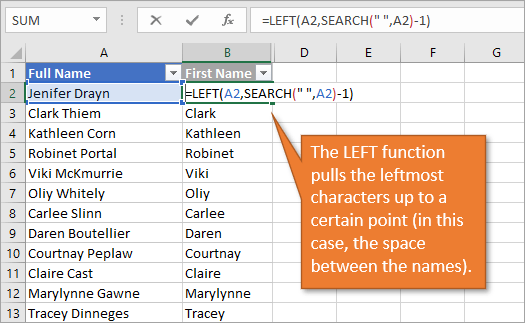
The LEFT Function
The LEFT function returns the specified number of characters from the start of a text string. To specify that number, we will use the value we just identified with the SEARCH function. The LEFT function will pull out the letters from the left of the Full Name column.
The LEFT function has two arguments.
- The first argument is text. That is just the cell that the function is pulling from—in our case A2.
- The second argument is [num_chars]. This is the number of characters that the function should pull. For this argument, we will use the formula we created above and subtract 1 from it, because we don’t want to actually include the space character in our results. So for our example, this argument would be SEARCH(” “,A2)-1
All together, our formula reads =LEFT(A2,SEARCH(” “,A2)-1)
Now that we’ve extracted the first name using the LEFT function, you can guess how we’re going to use the RIGHT function. It will pull out the last name. But before we go there, let me explain one of the components that we will need for that formula. That is the LEN function.
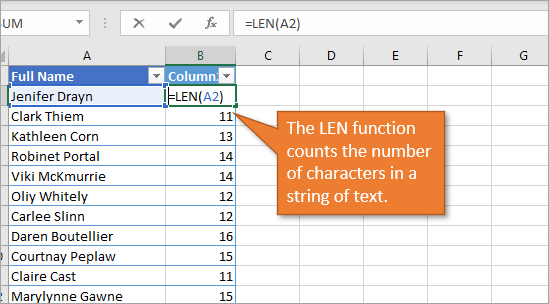
The LEN Function
LEN stands for LENGTH. This function returns the number of characters in a text string. In my name, there are 12 characters: 3 for Jon, 8 for Acampora, and 1 for the space in between.
There is only one argument for LEN, and that is to identify which text to count characters from. For our example, we again are using A2 for the Full Name. Our formula is simply =LEN(A2)
The RIGHT Function
The RIGHT formula returns the specified number of characters from the end of a text string. RIGHT has two arguments.
- The first argument is text. This is the text that it is looking through in order to return the right characters. Just as with the LEFT function above, we are looking at cell A2.
- The second argument is [num_chars]. For this argument we want to subtract the number of characters that we identified using the SEARCH function from the total number of characters that we identified with the LEN function. That will give us the number of characters in the last name.
Our formula, all together, is =RIGHT(A2,LEN(A2)-SEARCH(” “,A2))
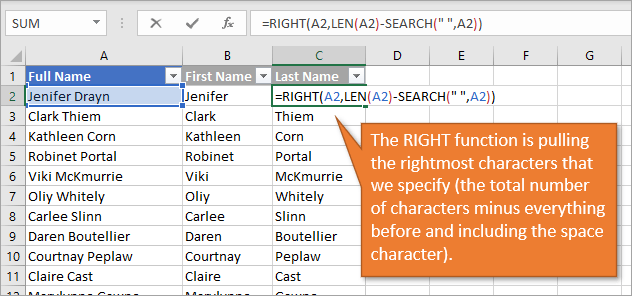
Note that we did not subtract 1 like we did before, because we want the space character included in the number that is being deducted from the total length.
Pros and Cons for Using Formulas to Split Cells
The one outstanding advantage to this method for splitting text is the automatic updates. When edits, additions, or deletions are made to the Full Name column, the First and Last names change as well. This is a big benefit compared to using Text to Columns, which requires you to completely repeat the process when changes are made. And even the Power Query method, though much simpler to update than Text to Columns, still requires a refresh to be manually selected.
Of course, one obvious disadvantage to this technique is that even though each of the four functions are relatively simple to understand, it takes some thought and time to combine them all and create formulas that work correctly. In other words, is not the easiest solution to implement of the three methods presented thus far.
Another disadvantage to consider is the fact that this only works for scenarios that have two names in the Full Name column. If you have data that includes middle names or two first names, the formula method isn’t helpful without making some considerable modifications to the formulas. (Homework challenge! If you’d like to give that a try, please do so and let us know your results in the comments.) As we saw in the Power Query tutorial, you do in fact have the capability to pull out more than two names with that technique.
Here are the links to the other posts on ways to split text:
- Split Cells with Text to Columns in Excel
- How to Split Text in Cells with Flash Fill in Excel
- How to Split Cells and Text in Excel with Power Query
- Split by Delimiter into Rows (and Columns) with Power Query
Conclusion
I hope you’ve learned something new from this post and that is helpful as you split data into separate columns. If you have questions or remarks, please leave a comment below!
One scenario is where you need to join multiple strings of text into a single text string. The flip of that is splitting a single text string into multiple text strings. If the data at hand was copied from somewhere or created by someone who completely missed the point of Excel columns, you will find that you need to split a block of text to categorize it.
Splitting the text largely depends on the delimiter in the text string. A delimiter is a character or symbol that marks the beginning or end of a character string. Examples of a delimiter are a space character, hyphen, period, comma.
 1")
Our example case for this guide involves splitting book details into book title, author, and genre. The delimiter we’ve used is a comma:
 2")
This tutorial will teach you how to split text in Excel with the Text to Columns and Flash Fill features, formulas, and VBA. The formulas method includes splitting text by a specific character. That’s the menu today.
Let’s get splitting!
Using Text to Columns
This feature lives up to its name. Text to Columns splits a column of text into multiple columns with specified controls. Text to Columns can split text with delimiters and since our data contains only a comma as the delimiter, using the feature becomes very easy. See the following steps to split text using Text to Columns:
- Select the data you want to split.
- Go to the Data tab and select the Text to Columns icon from the Data Tools
 3")
- Select the Delimited radio button and then click on the Next
 4")
- In the Delimiters section, select the Comma
- Then select the Next button.
 5")
- Now you need to choose where you want the split text. Click on the Destination field, then select the destination cell on the worksheet in the background where you want the split text to start.
- Select the Finish button to close the Text to Columns
 6")
Using the comma delimiter to separate the text string, Text to Columns has split the text from our example case into three columns:
 7")
Luckily, our data doesn’t contain a book with commas in the book name. If we had the book Cows, Pigs, Wars and Witches by Marvin Harris in the dataset, the text would be split into 5 columns instead of 3 like the rest. If the delimiter in your data is appearing in the text string for more than delimiting, you’ll have better luck splitting text with other methods. Now unto another observation.
Using TRIM Function to Trim Extra Spaces
Let’s cast a closer look at the output of Text to Columns. Notice how the last two columns carry one leading space? You can see that the values in columns D and E are not a hundred percent aligned to the left:
 8")
The last two columns carry a leading space because Text to Columns only takes the delimiter as a mark from where to split the text. The space character after the comma is carried with the next unit of text and that has our data with a leading space.
A quick fix for this is to use the TRIM function to clear up extra spaces. Here is the formula we have used to remove leading spaces from columns D and E:
=TRIM(C4)
The TRIM function removes all spaces from a text string other than a single space character between two words. Any leading, trailing, or extra spaces will be removed from the cell’s value. We have simply used the formula with a reference of the cell containing the leading space.
And that cleaned up the leading spaces for us. Data – good to go!
 9")
Using Formula To Separate Text in Excel
We can make use to Excel functions to construct formulas that can help us in splitting a text string into multiple.
Split String with Delimiter
Using a formula can also split a single text string into multiple strings but it will require a combo of functions. Let’s have a little briefing on the functions that make part of this formula we will use for splitting text.
The SUBSTITUTE function replaces old text in a text string with new text.
The REPT function repeats text a given number of times.
The LEN function returns the number of characters in a text string.
The MID function returns a given number of characters from the middle of a text string with a specified starting position.
The TRIM function removes all spaces, other than single spaces between words, from a text string.
Now let’s see how these functions combined can be used to split text with a single formula:
=TRIM(MID(SUBSTITUTE($B5,",",REPT(" ",LEN($B5))),(C$4-1)*LEN($B5)+1,LEN($B5)))
In our example, the first cell we are using this formula on is cell B5. The number of characters in B5 as counted by the LEN function is 49. The REPT function repeats spaces (denoted by “ “ in the formula) in B5 for the number of characters supplied by the LEN function i.e. 49.
The SUBSTITUTE function replaces the commas “,” in B5 with 49 space characters supplied by the REPT function. Since there are two commas in B5, one after the book name and one after the author, 49 spaces will be entered after the book name and 49 spaces after the author, creating a decent gap between the text we want to split.
Now let’s see the calculations for the MID function. The first bit is (C$4-1). In row 4, we added serial numbering for each of the columns for our categories. The row has been locked in the formula with a $ sign so the row doesn’t change as the formula is copied down. But we have left the column free so that the serial number changes for the respective columns used in the formula.
In the formula, 1 is subtracted from C4 (1-1=0) and the result is multiplied by the number of characters in B5 i.e. LEN($B5) and then 1 is added to the expression. The calculation for the starting position in the MID function, i.e. (C$4-1)*LEN($B5)+1, becomes (1-1)*49+1 which equals 1.
The MID function returns the text from the middle of B5, the starting position is 1 (that means the text to be returned is to start from the first character) and the number of characters to be returned is LEN($B5) i.e 49 characters. Since we have added 49 spaces in place of each of the commas, that gives us plenty of area to safely return just one chunk of text along with some extra spaces. The result up until the MID function is A Song of Ice and Fire with lots of trailing spaces.
The extra spaces are no problem. The TRIM function cleans any extra spaces leaving the single spaces between words and so we finally have the book name returned as A Song of Ice and Fire.
 10")
Now for the next column and hence the next category, the calculation for the starting position in the MID function will change like so (D$4-1)*LEN($B5)+1. The expression comes down to (2-1)*49+1 which equals 50. If the MID function is to return characters starting from the 50th character, with all the extra spaces added by the REPT function, what the MID function will return will be along this pattern: spaces author spaces.
The leading and trailing spaces will be trimmed by the TRIM function and the result will be George RR Martin.
 11")
The “+1” in the starting position argument of the MID function has no relevance for the subsequent columns, only for the first. That is because, without the “+1” in the first column’s calculation, it would be 0*49 which will end up in a #VALUE! error.
The formula copied along column E gives us the genre from the combined text in column B and that completes our set.
Split String at Specific Character
If there is only a single delimiter that is a specific character, such a lengthy formula as above will not be required to split the text. Let’s say, like our case example below, we are to split product code and product type which is joined by a hyphen.
Now this would be easier if the product code had a fixed number of characters; we would only have to use the LEFT function to return a certain number of characters. But what’s the fun in that?
We are going to let the FIND function do a bit of search work for us and find the hyphen in the text so the LEFT function and RIGHT function can return the surrounding text. This is the formula with the LEFT function for returning the first extract:
=LEFT(B3,FIND("-",B3)-1)
The FIND function searches B3 for the position of the hyphen “-“ in the text string, which is 6. The LEFT function then returns the characters starting from the left of the text and the number of characters to return is 6-1. “-1” at the end ensures that the characters returned do not include the hyphen itself. Here are the results of this formula for returning the first segment of split text:
 12")
Now for the second segment of text, the RIGHT function comes into play with this formula:
=RIGHT(B3,LEN(B3)-FIND("-",B3))
The FIND function is again used to find the location of the hyphen in B3 which we know is the 6th character. The LEN function returns the number of characters in B3 as 23. The RIGHT function extracts 23-6 characters from B3 and returns the product type “Bluetooth Speaker”. This is how it has worked for our example:
 13")
Using Flash Fill
The Flash Fill feature in Excel automatically fills in values based on a couple of manually provided examples. The ease of Flash Fill is that you need not remember any formulas, use any wizards, or fiddle with any settings. If your data is consistent, Flash Fill will be the quickest to pick up on what you are trying to get done. Let’s see the steps for using Flash Fill to split text and how it works for our example case:
- Type the first text as an example for Flash Fill to pick up the pattern and press the Enter
 14")
- From the Home tab’s Editing group, click on the Fill icon and select Flash Fill from the menu.
- Alternatively, use the shortcut keys Ctrl + E.
 15")
- Picking up on the provided example, Flash Fill will split the text and fill the column according to the same pattern:
 16")
- Repeat the same steps for each column to be Flash-Filled.
 17")
Flash Fill will save the trouble of having to trim leading and trailing spaces but as mentioned, if there are any anomalies or inconsistencies in the data (e.g a space before and after the comma), Flash Fill won’t be a reliable method of splitting text and due to the bulk of the data, the problem may go ignored. If you doubt the data to have inconsistencies, use the other methods for splitting the text.
Using VBA Function
The final method we will be discussing today for splitting text will be a VBA function. In order to automate tasks in MS Office applications, macros can be created and used with VBA. Our task is to split text in Excel and below are the steps for doing this using VBA:
- If you have the Developer tab added to the toolbar Ribbon, click on the Developer tab and then select the Visual Basic icon in the Code group to launch the Visual Basic
- You can also use the Alt + F11 keys.
 18")
- The Visual Basic editor will have opened:
 19")
- Open the Insert tab and select Module from the list. A Module window will open.
 20")
- In the Module window, copy-paste the following code to create a macro titled SplitText:
Sub SplitText()
Dim MyArray() As String, Count As Long, i As Variant
For n = 4 To 16
 MyArray = Split(Cells(n, 2), ",")
 Count = 3
 For Each i In MyArray
 Cells(n, Count) = i
 Count = Count + 1
 Next i
Next n
End Sub
Edit the following parts of the code as per your data:
- ‘For n = 4 To 16’ – 4 and 16 represent the first and last rows of the dataset.
- ‘MyArray = Split(Cells(n, 2), «,»)’ – The comma enclosed with double quotes is the delimiter.
- ‘Count = 3’ – 3 is the column number of the first column that the resulting data will be returned in.
 21")
- To run the code, press the F5
The data will be split as per the supplied values:
- Clean up the leading spaces in columns D and E using the TRIM function:
Now let’s split the active guide from its conclusion. Today you learned a few ways on how to split text in Excel. If you find yourself splitting hairs on your ability to split text next time, pocket this one and be ready to give it a go! We’ll be back with more Excel-ness to fill your pockets. Make some space!
Do you have any tricks on how to split columns in excel? When working with Excel, you may need to split grouped data into multiple columns. For instance, you might need to separate the first and last names into separate columns.
With Excel’s “Text to Feature” there are two simple ways of splitting your columns. If there is an evident delimiter such as a comma, use the “Delimited” option. However, the “Fixed method is ideal for splitting the columns manually.”
To learn how to split a column in excel and make your worksheet easy-to-read, follow these simple steps. You can also check our Microsoft Office Excel Cheat Sheet here. But, first, why should you split columns in excel?
Jump to:
- Why you need to split cells
- How do you split a column in excel?
- Method 1- Delimited Option
- Method 2- Fixed Width
- How to Split One Column into Multiple Columns in Excel
- Method 3- Split Columns by Flash Fill
- Method 4- Use LEFT, MID and RIGHT text string functions
Why you need to split cells
If you downloaded a file that Excel can’t divide, then you need to separate your columns. You should split a column in excel if you want to divide it with a specific character. Some examples of familiar characters are commas, colons, and semicolons.
How do you split a column in excel?
Method 1- Delimited Option
This option works best if your data contains characters such as commas or tabs. Excel only splits data when it senses specific characters such as commas, tabs, or spaces. If you have a Name column, you can separate it into First and Last name columns
- First, open the spreadsheet that you want to split a column in excel
- Next, highlight the cells to be divided. Hold the SHIFT key and click the last cell on the range
- Alternatively, right-click and drag your mouse to highlight the cells
- Now, click the Data tab on your spreadsheet.
- Navigate to and click on the “Text to Columns” From the Convert Text to Columns Wizard dialog box, select Delimited and click “Next.”
- Choose your preferred delimiter from the options given and click “Next.”
- Now, highlight General as your Column Data Format
- “General” format converts all your numeric values to numbers. Date values are converted to dates, and the rest of the data is converted to text. “Text” format only converts the data into text. “Date” allows you to select your desired date format. You can skip the column by choosing “Do not import column.”
- Afterward, type the “Destination” field for your new column. Otherwise, Excel will replace the initial data with the divided data
- Click “Finish” to split your cells into two separate columns.
Method 2- Fixed Width
This option is ideal if spaces separate your column data fields. So, Excel splits your data based on the character counts, be it 5th or 10th characters.
- Open your spreadsheet and select the column you wish to split. Otherwise, the “Text Columns” will be inactive.
- Next, click Text Columns in the “Data” Tab
- Click Fixed Width and then Next
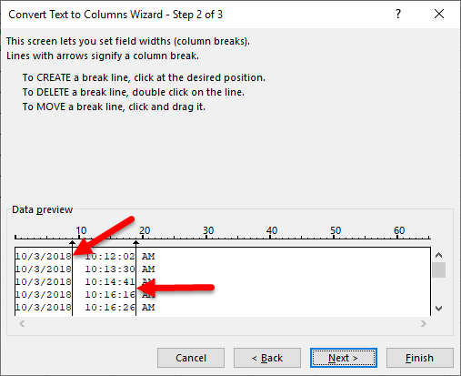
- Now you can adjust your column breaks in the “Data preview.” Unlike the “Delimited” option that focuses on characters, in “Fixed Width,” you select the position of splitting the text.
- Tips: Click the preferred position to CREATE a line break. Double-Click on the line to delete it. Click and drag a column break to move it
- Click Next if you’re satisfied with the results
- Select your preferred Column Data Format
- Next, type the “Destination” field for your new column. Otherwise, Excel will replace the initial data with the divided data.
- Finally, click Finish to confirm the changes and divide your column into two
How to Split One Column into Multiple Columns in Excel
A single column can be split into multiple columns using the same steps outlined in this guide
Tip: The number of columns depends on the number of delimiters that you select. For instance, Data will be split into three columns if it contains three commas.
Method 3- Split Columns by Flash Fill
If you are using Excel 2013 and 2016, you are in luck. These versions are integrated with a Flash fill feature that extracts data automatically once it recognizes a pattern. You can use flash fill to split the first and last name in your column. Alternatively, this feature combines separate columns into one column.
If you don’t have these professional versions, quickly upgrade your Excel version. Follow these steps to divide your columns using Flash Fill.
- Assume your data resembles the one in the image below

- Next, in cell B2, type the First Name as below

- Navigate to the Data Tab and click Flash Fill. Alternatively, use the shortcut CTRL+E
- Selecting this option automatically separates all the First Names from the given column
Tip: Before clicking Flash Fill, ensure that cell B2 is selected. Otherwise, a warning appears that
- Flash Fill cannot recognize a pattern to extract the values. Your extracted values will look like this:

- Apply the same steps for the last name as well.

Now, you have learned to split a column in excel into multiple cells
Method 4- Use LEFT, MID and RIGHT text string functions
Alternatively, use LEFT, MID, and RIGHT string functions to split your columns in Excel 2010, 2013 and 2016.
- LEFT function: Returns the first character or characters on your left, depending on the specific number of characters you require.
- MID Function: Returns the middle number of characters from string text beginning from where you specify.
- RIGHT Function: Gives the last character or characters from your text field, depending on the specified number of characters on your right.
However, this option is not valid if your data contains a formula such as VLOOKUP. In this example, you’ll learn how to split Address, City, and zip code columns.

To extract the Addresses using the LEFT function:
- First select cell B2
- Next, apply the formula =LEFT(A2,4)
Tip: 4 represents the number of characters representing the address
3. Click, hold and drag down the cell to copy the formula to the entire column

To extract the City data, use the MID function as follows:
- First, Select cell C2
- Now, apply the formula =MID(A2,5,2)
Tip: 5 represents the fifth character. 2 is the number of characters representing the city.
- Right-click and drag down the cell to copy the formula in the rest of the column
Finally, to extract the last characters in your data, use the Right text function as follows:
- Select Cell D2
- Next, apply the formula =RIGHT(A2,5)
Tip: 5 represents the number of characters representing the Zip Code
- Click, hold and drag down the cell to copy the formula in the entire column

Tips to remember
- The shortcut key for Flash Fill is CTRL+E
- Always try to identify a shared value in your column before splitting it
- Familiar characters when splitting columns include commas, tabs, semicolons, and spaces.
Text Columns is the best feature to split a column in excel. It might take you several attempts to master the process. But once you get the hang of it, it will only take you a couple of seconds to split your columns. The results are professional, clean, and eye-catching columns.
If you’re looking for a software company you can trust for its integrity and honest business practices, look no further than SoftwareKeep. We are a Microsoft Certified Partner and a BBB Accredited Business that cares about bringing our customers a reliable, satisfying experience on the software products they need. We will be with you before, during, and after all the sales.
Separating Text in Excel
The texts in Excel can appear in different ways. For example, maybe there is a text joined by some symbol, or it is like a first name and the last name.
At some point in our life, we will want those texts separated. The problem statement is explained above that we will come towards some data where we need to separate those texts from one another. But how do we separate those texts from one another? There is one very basic way to do it: copy the desired text in each selected individual cell. Else, we can use some pre-given Excel tools to perform.
Table of contents
- Separating Text in Excel
- How to Separate Text in Excel?
- Example #1 – Delimiter Method to Separate Text
- Example #2 – Using the Fixed Width Method to Separate Text
- Example #3 – Using Formulas for Separating Text
- Things to Remember in Separating Text in Excel (text to column & formula)
- Recommended Articles
- How to Separate Text in Excel?
How to Separate Text in Excel?
There are two methods to separate Texts in Excel:
- Using “Text to Columns in ExcelText to columns in excel is used to separate text in different columns based on some delimited or fixed width. This is done either by using a delimiter such as a comma, space or hyphen, or using fixed defined width to separate a text in the adjacent columns.read more“: It further has its own two bifurcations:
- Delimited: This feature splits the text, which is joined by characters, commas, tabs, spaces, semicolons, or any other character such as a hyphen (-).
- Fixed Width: This feature splits the text, which is joined with spaces with a certain width.
- Using Excel Formulas: We can use formulas like the Len in excelThe Len function returns the length of a given string. It calculates the number of characters in a given string as input. It is a text function in Excel as well as an inbuilt function that can be accessed by typing =LEN( and entering a string as input.read more to calculate the length of the string and separate the values by knowing the position of the characters
Let us learn these methods using examples.
You can download this Separate Text Excel Template here – Separate Text Excel Template
Example #1 – Delimiter Method to Separate Text
First, where do we find this feature text to columns in Excel? It is under the “Data” tab in the “Data Tools” section.
Consider the following data,
We want to separate the first and last names. Therefore, the last names’ content is in the B column.
Below are the steps of separating text in excel –
- First, we must select the column containing the data, A column.

- Under the “Data” tab in the “Data Tools” section, click on “Text to Columns.”

- A dialog box appears for text to columns wizard.

- As we will use the delimiter method first, select the “Delimited” option and click on “Next.” Another dialog box appears.
- Our texts are separated in Excel by spaces for the current data, so select the “Space” option as a “delimiter” ( By default, Excel selects a tab as a delimiter). Then, finally, click on “Next.”
- Our “Data preview” shows that our texts are separated with first and last names. Click on “Finish” to see the result.
- We have successfully separated our Excel text by using the text-to-column delimiter method.

Example #2 – Using the Fixed Width Method to Separate Text
We already know where the option of text to the column is in Excel. It is in the “Data” tab under the “Data Tools” section.
Now we consider the following data,
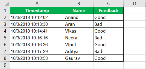
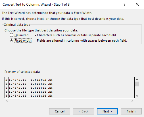
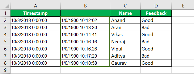
There is a survey company that is surveying for the feedback of a restaurant. The users give their feedback as “Good” or “Bad.” But every response is saved by a timestamp, which means with every response, time is recorded, specific data and time in hours and minutes.
We need to separate the date from the time in the data. Below is the data.
Step #1 – We need to separate the contents of column A, but there is data in column B, so we need to insert another column between columns A and B. Select column B and press the “CTRL + +” keys for that.
It adds another column between the columns and shifts the data from previous column B to column C.
Step #2 – Now, select the data in column A. Click on “Text to Columns” under the “Data” tab in the “Data Tools” section.
A dialog box appears for converting text to columns wizard.
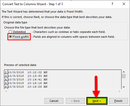
Step #3 – This time, we use a fixed width method. So ensure that the “Fixed width” method option is selected and click on “Next.” Another “Convert Text to Column Wizard” dialog box appears.
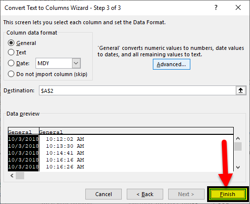
Step #4 – In the “Data preview,” we can see that the data is separated into three parts: date, time, and the meridian, AM, and PM.
We need only date and time, so hover the mouse around the second line and double click on it, and it disappears.
Step #5 – Now, click “Next.” Another “Convert Text to Columns Wizard” dialog box appears. Then, you need to click on the “Finish” button.
Now, the data is separated with date in one column and time in another.
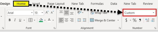
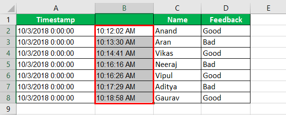
Step #6 – The data formatting in column B is incorrect, so we must rectify it. Select the contents on column B, and in the “Home” tab under the “Number” section, the default selection is “Custom.” We need to change it to “Time.”
Step #7 – We have successfully separated our Excel data using the “Text to Columns Fixed Width” method.
Example #3 – Using Formulas for Separating Text
We can also use Excel formulas to separate the text and numbers, which are joined together. Then, we can remove that data by using “Text to Columns.” However, we use formulas for complex situations.
Let us consider the following Data:
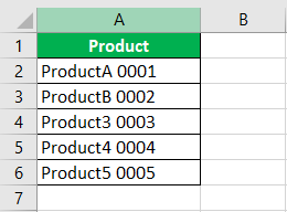
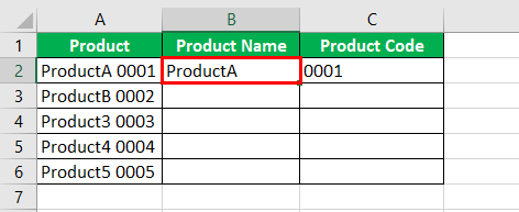
We have products in column A with their respective product codes. We need products in one column and product code in another. We want to use formulas to do this.
Step #1- To this, we must first count the number of digits and separate that number from the character.
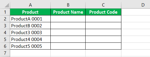
Step #2- We need the “Product Name” in column B and “Product Code” in column C.
Step #3- First, we will separate the digits to separate the text in Excel from the data. In C2, write the following Excel formula to separate text.
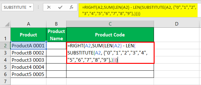
We use the right to function as we know the numbers are in the right.
Step #4- Now, in Cell B2, write the following Formula,
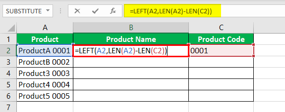
Step #5- Press the “Enter” key. Using the LEN function, we have successfully separated our data from “Product Name” and ” Product Code.”
Step #6- Drag the formulas to cells B6 and C6, respectively.
Things to Remember in Separating Text in Excel (text to column & formula)
- If we use the “Text to Columns” method, always ensure that we have an additional column so that the data in any column does not get replaced.
- We must ensure the characters’ positioning if we separate texts in Excel using Excel formulas.
Recommended Articles
This article is a guide to Separate Text in Excel. Here, we discuss how to separate text in Excel using two methods: 1) Text to Columns (delimited and fixed width), and 2) Excel formulas with practical examples and a downloadable template. You may learn more about Excel from the following articles: –
- Date to Text in ExcelYou can convert Date to Text in Excel through the most commonly used method, i.e., the text function or by using: Text-to-Column option, Copy Paste Method and VBA.
read more - Convert Date to Text in ExcelTo convert a date to text in Excel, right-click on the date cell and select the format cells option. A new window will open. You can convert the date to text by selecting the desired format from a list of options.read more
- Numbers to Text in Excel with ExamplesYou may need to convert numbers to text in Excel for a variety of reasons. If you use Excel spreadsheets to store long and not-so-long numbers, or if you don’t want the numbers in the cells to be involved in calculating, or if you want to display leading zeros in numbers in cells, you’ll need to convert them to text at some point. It’s useful for displaying numbers in a more readable format or combining numbers with text or symbols. The methods listed below can be used to accomplish this.read more
- Top Excel Keyword Shortcuts