
Excel for Microsoft 365 Excel 2021 Excel 2019 Excel 2016 Excel 2013 More…Less
You might want to split a cell into two smaller cells within a single column. Unfortunately, you can’t do this in Excel. Instead, create a new column next to the column that has the cell you want to split and then split the cell. You can also split the contents of a cell into multiple adjacent cells.
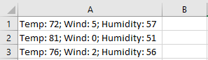
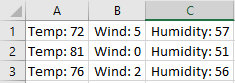
See the following screenshots for an example:
Split the content from one cell into two or more cells
-
Select the cell or cells whose contents you want to split.
Important: When you split the contents, they will overwrite the contents in the next cell to the right, so make sure to have empty space there.
-
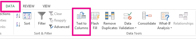
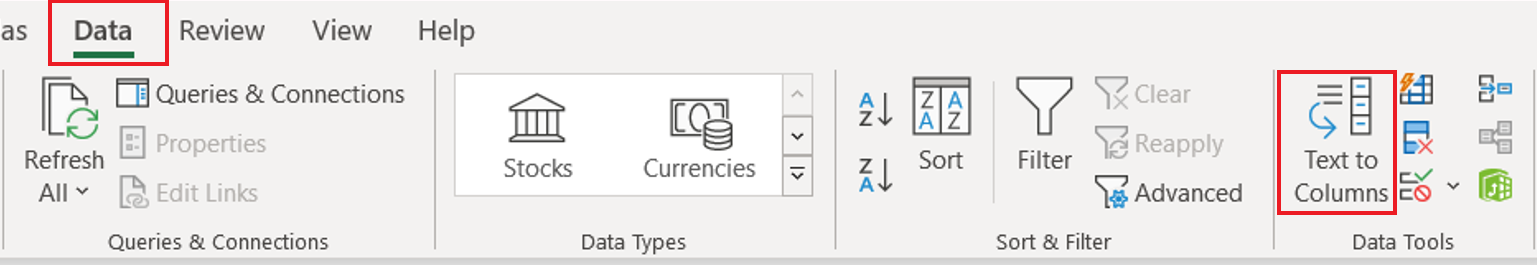
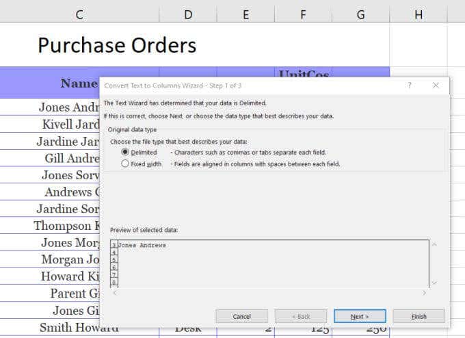
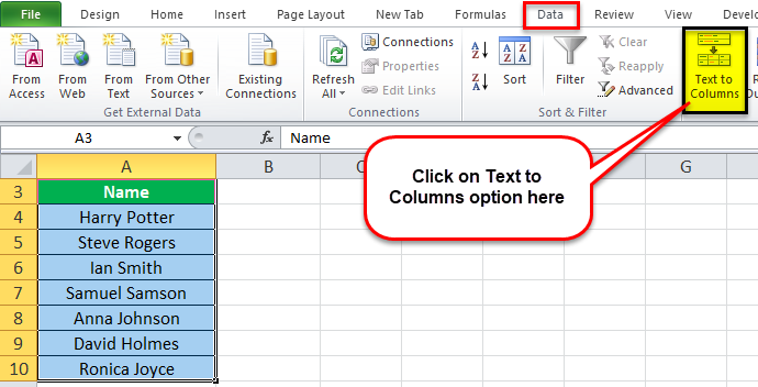
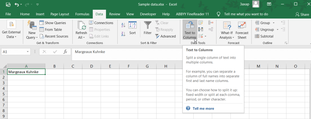
On the Data tab, in the Data Tools group, click Text to Columns. The Convert Text to Columns Wizard opens.

-
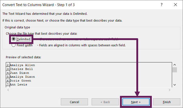
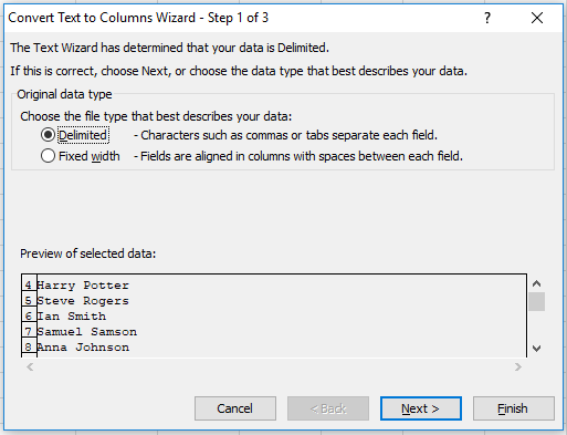
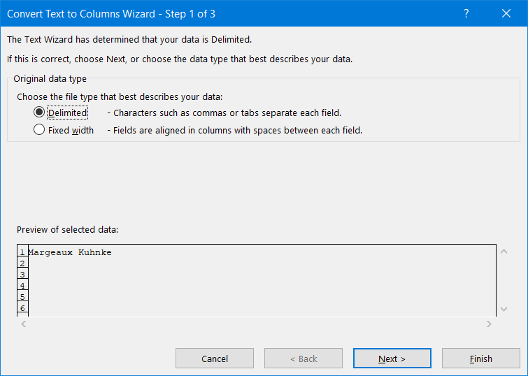
Choose Delimited if it is not already selected, and then click Next.
-
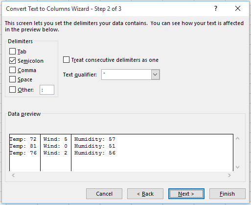
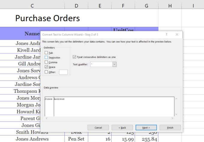
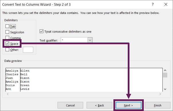
Select the delimiter or delimiters to define the places where you want to split the cell content. The Data preview section shows you what your content would look like. Click Next.
-
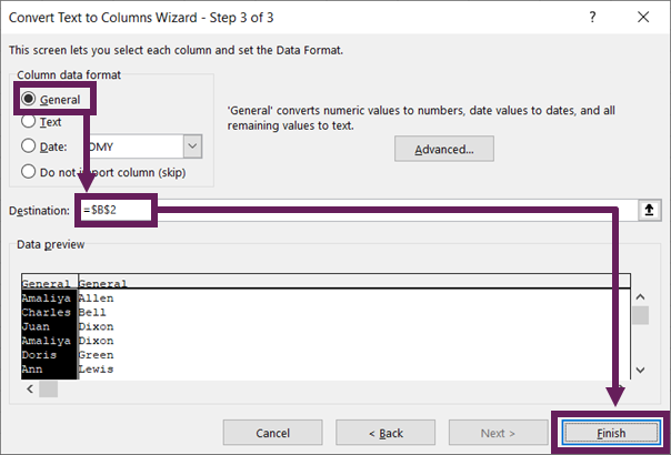
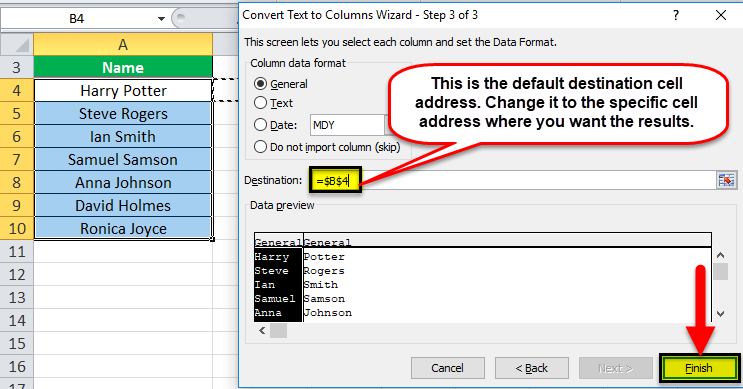
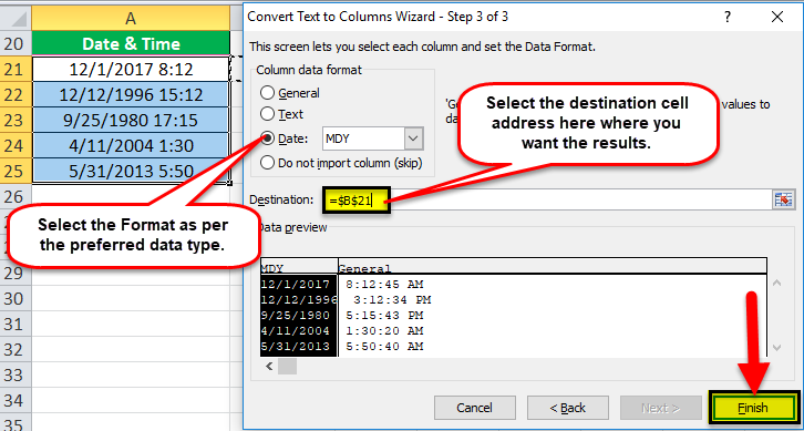
In the Column data format area, select the data format for the new columns. By default, the columns have the same data format as the original cell. Click Finish.
See Also
Merge and unmerge cells
Merging and splitting cells or data
Need more help?
Want more options?
Explore subscription benefits, browse training courses, learn how to secure your device, and more.
Communities help you ask and answer questions, give feedback, and hear from experts with rich knowledge.
There can be situations when you have to split cells in Excel. These could be when you get the data from a database or you copy it from the internet or get it from a colleague.
A simple example where you need to split cells in Excel is when you have full names and you want to split these into first name and last name.
Or you get address’ and you want to split the address so that you can analyze the cities or the pin code separately.
How to Split Cells in Excel
In this tutorial, you’ll learn how to split cells in Excel using the following techniques:
- Using the Text to Columns feature.
- Using Excel Text Functions.
- Using Flash Fill (available in 2013 and 2016).
Let’s begin!
Split Cells in Excel Using Text to Column
Below I have a list of names of some of my favorite fictional characters and I want to split these names into separate cells.:

Here are the steps to split these names into the first name and the last name:
- Select the cells in which you have the text that you want to split (in this case A2:A7).
- Click on the Data tab
- In the ‘Data Tools’ group, click on ‘Text to Columns’.
- In the Convert Text to Columns Wizard:

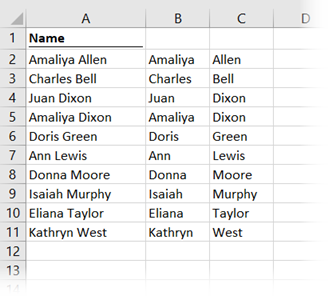
This will instantly split the cell’s text into two different columns.

Note:
- Text to Column feature splits the content of the cells based on the delimiter. While this works well if you want to separate the first name and the last name, in the case of first, middle, and last name it will split it into three parts.
- The result you get from using the Text to Column feature is static. This means that if there are any changes in the original data, you’ll have to repeat the process to get updated results.
Split Cells in Excel Using Text Functions
Excel Text functions are great when you want to slice and dice text strings.
While the Text to Column feature gives a static result, the result that you get from using functions is dynamic and would automatically update when you change the original data.
Splitting Names that have a First Name and Last Name
Suppose you have the same data as shown below:

Extracting the First Name
To get the first name from this list, use the following formula:
=LEFT(A2,SEARCH(" ",A2)-1)
This formula would spot the first space character and then return all the text before that space character:

This formula uses the SEARCH function to get the position of the space character. In the case of Bruce Wayne, the space character is in the 6th position. It then extracts all the characters to the left of it by using the LEFT function.
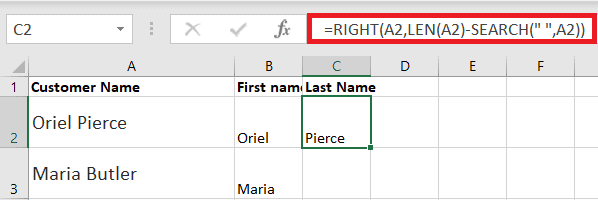
Extracting the Last Name
Similarly, to get the last name, use the following formula:
=RIGHT(A2,LEN(A2)-SEARCH(" ",A2))

This formula uses the search function to find the position of the spacebar using the SEARCH function. It then subtracts that number from the total length of the name (that is given by the LEN function). This gives the number of characters in the last name.
This last name is then extracted by using the RIGHT function.
Note: These functions may not work well if you have leading, trailing or double spaces in the names. Click here to learn how to remove leading/trailing/double spaces in Excel.
Splitting Names that have a First Name, Middle Name, and Last Name
There may be cases when you get a combination of names where some names have a middle name as well.

The formula in such cases is a bit complex.
Extracting the First Name
To get the first name:
=LEFT(A2,SEARCH(" ",A2)-1)
This is the same formula we used when there was no middle name. It simply looks for the first space character and returns all the characters before the space.
Extracting the Middle Name
To get the Middle Name:
=IFERROR(MID(A2,SEARCH(" ",A2)+1,SEARCH(" ",A2,SEARCH(" ",A2)+1)-SEARCH(" ",A2)),"")
MID function starts from the first space character and extracts the middle name by using the difference of the position of the first and the second space character.
In cases there is no middle name, the MID function returns an error. To avoid the error, it is wrapped within the IFERROR function.
Extracting the Last Name
To get the Last Name, use the below formula:
=IF(LEN(A2)-LEN(SUBSTITUTE(A2," ",""))=1,RIGHT(A2,LEN(A2)-SEARCH(" ",A2)),RIGHT(A2,LEN(A2)-SEARCH(" ",A2,SEARCH(" ",A2)+1)))
This formula checks whether there is a middle name or not (by counting the number of space characters). If there is only 1 space character, it simply returns all the text to the right of the space character.
But if there are 2, then it spots the second space character and returns the number of characters after the second space.
Note: These formula works well when you have names that have either the fist name and last name only, or the first, middle, and last name. However, if you have a mix where you have suffixes or salutations, then you’ll have to modify the formulas further.
Split Cells in Excel Using Flash Fill
Flash Fill is a new feature introduced in Excel 2013.
It could be really handy when you have a pattern and you want to quickly extract a part of it.
For example, let’s take the first name and the last name data:
Flash fill works by identifying patterns and replicating it for all the other cells.
Here is how you can extract the first name from the list using Flash Fill:
How Flash Fill Works?
Flash Fill looks for the patterns in the data set and replicates the pattern.
Flash Fill is a surprisingly smart feature and works as expected in most of the cases. But it also fails in some cases too.
For example, if I have a list of names that has a combination of names with some having a middle name and some don’t.
If I extract the middle name in such a case, Flash Fill will erroneously return the last name in case there is no first name.

To be honest, that’s still a good approximation of the trend. However, it is not what I wanted.
But it still is a good enough tool to keep in your arsenal and use whenever the need arises.
Here is another example where Flash Fill works brilliantly.
I have a set of addresses from which I want to quickly extract the city.

To quickly get the city, enter the city name for the first address (enter London in cell B2 in this example) and use the autofill to fill all the cells. Now use Flash Fill and will instantly give you the name of the city from each address.
Similarly, you can split the address and extract any part of the address.
Note that this would need the address to be a homogenous data set with the same delimiter (comma in this case).
In case you try and use Flash Fill when there is no pattern, it will show you an error as shown below:

In this tutorial, I have covered three different ways to split cells in Excel into multiple columns (using Text to Columns, formulas, and Flash Fill)
Hope you found this Excel tutorial useful.
You May Also Like the Following Excel Tutorials:
- How to Quickly Combine Cells in Excel.
- How to Extract a Substring in Excel Using Formulas.
- How to Count Cells that Contain Text Strings.
- Extract Usernames from Email Ids in Excel [2 Methods].
- How to Split Multiple Lines in a Cell into Separate Cells/Columns.
Note: This guide on how to split cells in Excel is suitable for all versions of Excel.
In your Excel journey, you will come across situations where you have to work with imported data. In these cases, it is very common to find cells of data that are not in the desired format.
For example, I have an Excel sheet, where a column of cells displays both the first and last names of customers together. But, I need to split the cells into two separate columns for the first and last names.
Related:
How To Find Duplicates In Excel? The Best Guide
Excel Goal Seek—the Easiest Guide (3 Examples)
Create A Pivot Table In Excel—the Easiest Guide
In other words, how to split cells across multiple columns?
In this guide, I’ll explain three easy ways to split cells in Excel with ample illustrations. You can watch this short video to easily learn how to split cells in Excel.
Please find below the sample Excel sheet to download and follow along with me.

- How to Split Cells in Excel Using Text to Column?
- How to Split Cells in Excel Using Text Functions?
- How to Split Cells Using Flash Fill (Auto Fill)?
- FAQs
How to Split Cells in Excel Using Text to Column?
One of the easiest ways to split cells is to use the text to column feature. To do this do the following:
- Select the column of cells you want to split. You can also select a specific range in a column.

- Locate and click on the Text to Columns button under the Data tab. It can be found in the Data Tools section.
- In the Convert Text to Columns Wizard, select the Delimited option as the data type.

Click Next.
- In the next window, select the Delimiters for splitting your cells. A delimiter is the character based on which the split should happen. In this case, the names have a space between them. Hence, the delimiter here is Space.
Also Read:
How To Use Excel Countifs: The Best Guide
Excel Conditional Formatting -the Best Guide (Bonus Video)
The Best Excel Project Management Template In 2021
Note that, any delimiter can be used if the data has it. If you are confused about which one to select, use trial and error to see how your split data appears in the Data preview window.
Click on Next.
- Now, choose your Data Type and Enter your Destination cell. In this example the destination cell is B2. keep in mind to leave sufficient space, especially if there are multiple delimiters in your data.

Click on Finish.
Congratulations, your cells have split into multiple cells. Keep in mind that this is not a dynamic feature. It means that any later change in the original names or data will not reflect in the result column.

How to Split Cells in Excel Using Text Functions?
Sometimes, you need a more robust solution to splitting cells. For example, the data may not contain a standard delimiter for you to choose. Or you may need to make the splitting process dynamic.
For such cases, use the Text functions to split the cells.
There are many text functions in Excel, but we don’t need all of them here. A few important ones are:
1. LEN – Returns the length of a string
2. RIGHT – Extract a specified number of characters from a String’s right end.
3. LEFT – Extract a specified number of characters from a String’s left end.
4. FIND – Look for a string inside another string.
5. SEARCH – Return the positions of a string inside another string
6. MID – Extract a specified number of characters from a String’s centre.
There is no one standard way to do this. You can use any combination of the above text functions to achieve your split.
Now, I’ll show you how to implement this using simple examples. Do the following:
- Determine the type of split you want in the data. I am using the same example, where the first names and last names are separated by a space.
- Now, to extract the first name, use a combination of SEARCH and LEFT functions.
Enter the formula =LEFT(A2,SEARCH(” “,A2)-1) in cell B2.
Here, the SEARCH looks for any space in the customer name and returns its position in the string. Then, the LEFT function extracts the part of the string from the left side, up to the position returned by the SEARCH function.

- Drag the formula to all the cells below.
You have successfully extracted the first names.
- Now, repeat the same process to extract the last names, except here, use the RIGHT function to extract from the end of the string.
Enter the formula =RIGHT(A2,LEN(A2)-SEARCH(” “,A2)) in cell C2.
Here, the SEARCH looks for any space in the customer name and returns its position in the string. Then, the RIGHT function extracts the part of the string from the right side, up to the position, returned by the SEARCH function.
Drag the formula to all the cells below.
- Congratulations, you have successfully split the first and last names.
- The most important thing to note here is that the split is dynamic. That is, when you change the source data, the results also change automatically.

How to Split Cells Using Flash Fill (Auto Fill)?
Sometimes, you may want to split cells without using any formula or wizard menus.
To do this, use the Flash Fill feature to split cells instantly.
Follow these simple steps to accomplish this:
1. Type in the neighbouring cell, in the next column, an example of the split cell.
2. Drag the fill handle till the end of the data range.
3. Click on the AutoFill Options button at the end of the range and select Flash Fill

Now, Excel will recognize the pattern and will fill the remaining cells for you. Repeat the same process for the last names. You have successfully split the cells.
Suggested Reads:
Create An Excel Dashboard In 5 Minutes – The Best Guide
Dynamic Dropdown Lists In Excel – Top Data Validation Guide
Predict Future Values Using Excel Forecast Sheet – The Best Guide
FAQs
How to split cells in Excel to extract data?
You can split cells in Excel using these three methods.
1. Use the Text to Column feature to split cells with delimiter.
2. Use Text functions to split cells if you need a dynamic split.
3. Use Flash Fill in the Auto Fill feature to automatically split strings in cells.
Is there a split function in Excel?
Yes, there is a SPLIT function in Excel, which uses a delimiter to split strings into smaller sub strings.
Let’s Wrap Up
In this guide, I have explained how to split cells in Excel in a step-by-step manner. I have covered all three important methods to split cells with detailed examples. If you have any doubts regarding splitting cells or any other Excel feature, please let us know in the comments below.
If you need more high-quality Excel guides, please check out our free Excel resources centre.
Simon Sez IT has been teaching Excel for over ten years. For a low, monthly fee you can get access to 100+ IT training courses. Click here for advance Excel courses with in-depth training modules.

Adam Lacey

Adam Lacey is an Excel enthusiast and online learning expert. He combines these two passions at Simon Sez IT where he wears a number of different hats.When Adam isn’t fretting about site traffic or Pivot Tables, you’ll find him on the tennis court or in the kitchen cooking up a storm.
If you’re working with data in Excel that you’ve imported from other sources, sometimes you have to work with data that isn’t in a format that you want. This is especially true with comma-delimited text that comes into single cells.
The only way to deal with that data is to split a cell in Excel. There are different ways to do this, depending on the format of the data.

In this article you’ll learn how to split a cell, how to roll that out to an entire column, and when you should choose each option.
Convert Text To Columns
One of the most common methods to split a cell in Excel is using the Text to Columns tool. This lets you split an entire column of cells using whatever rules you like.
The feature also includes an easy-to-use wizard, which is why most people prefer using it. It also handles any text format, whether the separating text is a space, a tab, or a comma.
Let’s look at an example of how to use the Text to Columns feature in Excel.
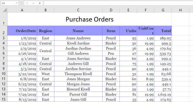
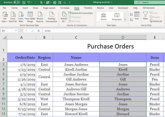
In this example, we want to split the Name column into two cells, the first name and the last name of the salesperson.
To do this:
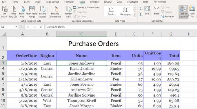
1. Select the Data menu. Then select Text to Columns in the Data Tools group on the ribbon.
2. This will open a three-step wizard. In the first window, make sure Delimited is selected and select Next.
3. On the next Wizard window, deselect Tab and make sure Space is selected. Select Next to continue.
4. On the next window, select the Destination field. Then, in the spreadsheet, select the cell where you want the first name to go. This will update the cell in the Destination field to where you’ve selected.
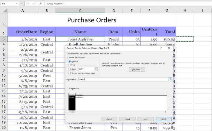
5. Now, select Finish to complete the Wizard.
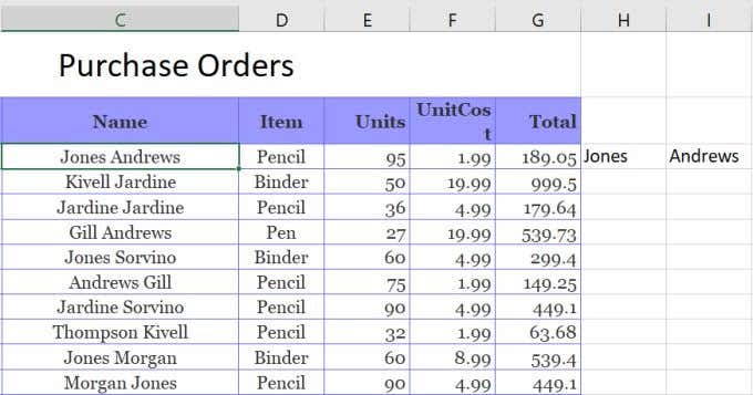
You’ll see that the single cell that contained both the first name and last name has been split into two cells that contain each one individually.
Note: The process above works because the data to split in the cell had a space separating the text. This text-to-column feature can also handle splitting a cell in Excel if the text is separated by a tab, semicolon, comma, or any other character you specify.
Use Excel Text Functions
Another way to split a cell in Excel is by using different text functions. Text functions let you extract pieces of a cell that you can output into another cell.
Text functions in Excel include:
- Left(): Extract a number of characters from the left side of the text
- Right(): Extract a number of characters from the right side of the text
- Mid(): Extract a number of characters from the middle of a string
- Find(): Find a substring inside of another string
- Len(): Return the total number of characters in a string of text
To split cells, you may not need to use all of these functions. However, there are multiple ways you can use these to accomplish the same thing.
For example, you can use the Left and Find function to extract the first name. The Find function helps because it can tell you where the delimiting character is. In this case, it’s a space.
So the function would look like this:
=LEFT(C3,FIND(” “,C3))
When you press enter after typing this function, you’ll see that the first name is extracted from the string in cell C3.
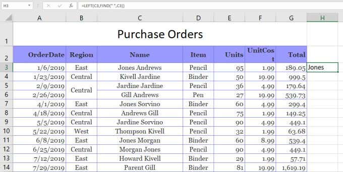
This works, because the Left function needs the number of characters to extract. Since the space character is positioned at the end of the first name, you can use the FIND function to find the space, which returns the number of characters you need to get the first name.
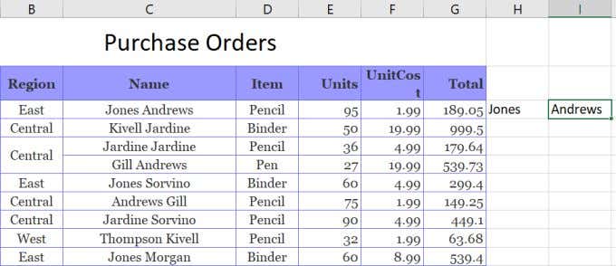
You can extract the last name either using either the Right function or the Mid function.
To use the Right function:
=RIGHT(C3,LEN(C3)-FIND(” “,C3))
This will extract the last name by finding the position of the space, then subtracting that from the length of the total string. This gives the Right function the number of characters it needs to extract the last name.
Technically, you could do the same thing as the Right function using the Mid function, like this:
=MID(C3,FIND(” “,C3),LEN(C3)-FIND(” “,C3))
In this case the Find function gives the Mid function the starting point, and the Len combined with Find provides the number of characters to extract. This will also return the last name.
Using Excel text functions to split a cell in Excel works as well as the Text-To-Column solution, but it also lets you fill the entire column beneath those results using the same functions.
Split Cell in Excel Using Flash Fill
The last option to split a cell in Excel is using the Flash Fill feature. This requires that the cells you’re splitting the original one into are right beside it.
If this is the case, all you have to do is type the part of the original cell that you want to split out. Then drag the lower right corner of the cell down to fill the cell beneath it. When you do this, you’ll see a small cell fill icon appear with a small plus sign next to it.
Select this icon and you’ll see a menu pop-up. Select Flash Fill in this menu.
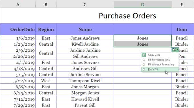
When you do this, you’ll see that the Flash Fill feature automatically detects why you typed what you typed, and will repeat the process in the next cell. It’ll do this by detecting and filling in the first name in the original cell to the left.
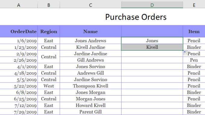
You can actually do this same procedure when you fill the entire column. Select the same icon and select Flash Fill. It’ll fill the entire column with the correct first name from the cells to the left.
You can then copy this entire column and paste it into another column, then repeat this same process to extract the last names. Finally, copy and paste that entire column where you want it to go in the spreadsheet. Then delete the original column you used to perform the Flash Fill process.
Splitting Cells in Excel
As you can see there are a few ways to accomplish the same thing. How you split a cell in Excel boils down to where you want the final result to go and what you plan to do with it. Any options works, so choose the one that makes the most sense for your situation and use it.
There are many circumstances where we receive information with multiple data points inside a single cell. This often occurs when the data’s original intention is slightly different from how we intend to use it. In these circumstances, we often need to split a cell into its constituent parts. This post will look at solving this problem and learn how to split cells in Excel.
The scenario we are trying to solve is; we want to split an individual’s full name into the first name and last name components.
If we have ten cells, it’s not a big problem; we can do that manually by entering each value into a separate column. But if we have hundreds or thousands of cells, we need to find another way. Thankfully we can turn to a variety of Excel features.
Download the example file
I recommend you download the example file for this post. Then you’ll be able to work along with examples and see the solution in action, plus the file will be useful for future reference.
![]()
Download the file: 0051 Split cells in Excel.xlsx
Watch the video
Watch the video on YouTube.
Example data
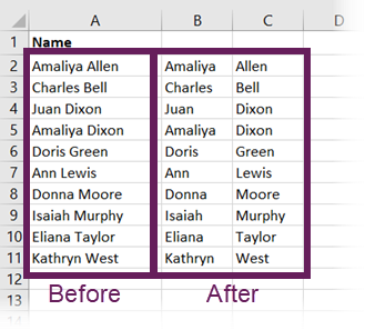
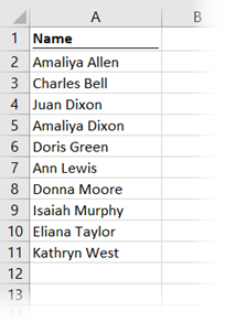
In all our solutions, we will be using the following data set.
In this post, we are covering 4 possible options. Depending on your data, one method may lead to better results than others. The lower the level of data consistency, the harder the process becomes.
Split cells using Text to Columns Wizard
Text to columns is a feature in Excel that hides in plain sight. It’s on the ribbon as an icon, but unless you know it’s there and what it does, you may not have used it before.
The steps to split a cell into multiple columns with Text to Columns are:
- Select the cell or cells containing the text to be split
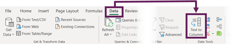
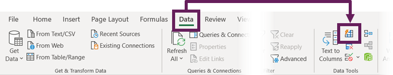
- From the ribbon, click Data > Data Tools (Group) > Text to Columns

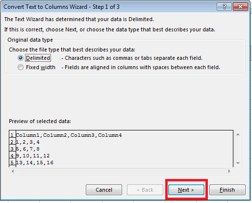
- The Convert Text to Columns Wizard dialog box will open
- Select the Delimited option. This allows us to split the text at each occurrence of specific characters. In our case, the space character is our delimiter. Click Next.

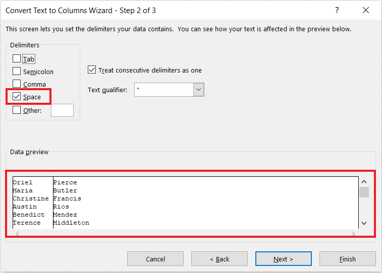
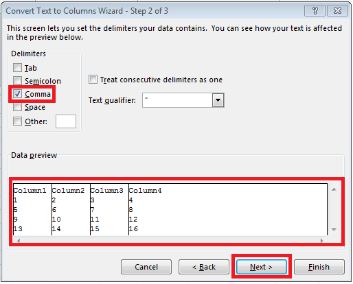
- Step 2 in the Convert Text to Columns Wizard opens. In the Delimiters group, select the relevant option for your scenario. I have selected Space for this scenario. Click Next.

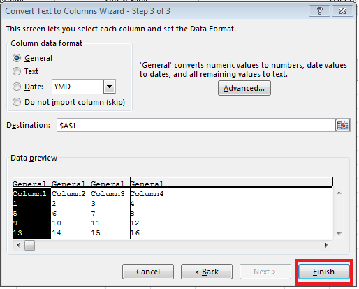
- Finally, in Step 3 of the Text to Columns Wizard, we specify the format for the result. As we are using text, the General format is a reasonable option. Select a Destination cell where to output the result. I have selected Cell B2. Click Finish.

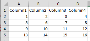
That’s it. Just a few clicks and we’re done 🙂
Our range should now be perfectly split into multiple columns.
Note about Text to Columns
Text to columns is not a dynamic feature; if the source cells change, we need to re-run the process by going back to Data > Data Tools (Group) > Text to Columns.
Text to columns works best on cells that are in a consistent format. For example, if one cell had 1 space, while others had 2 spaces, it may not provide the desired results.
Split cells using Flash Fill
Flash Fill is a fantastic feature that was introduced in Excel 2013. You may have already used it without even being aware of it. It is very easy to use for splitting cells in Excel with simple patterns.
It can run in two ways:
- In the background, Excel tries to find patterns in the text and automatically makes suggestions.
- Triggered by the user at specific times
Background execution
For background execution:
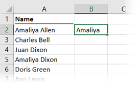
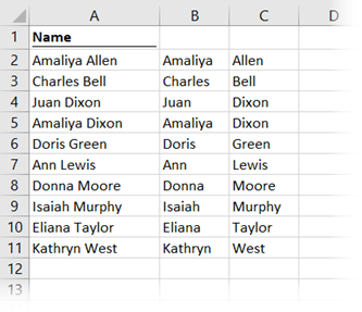
- With the source cells on the left, type the text element we want to extract in the first row of the first column (cell B2 in the screenshot below).

Nothing will happen yet. - Start typing the element of the text we want to extract from the second cell. Now Flash Fill jumps into action and makes recommendations:

- Press the Tab or Enter key to accept the recommended fill.
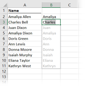
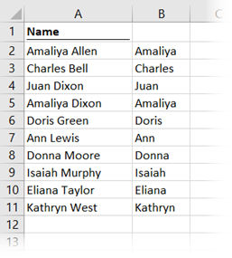
This gives us the first name.
Manual execution
Now let’s manually trigger Flash Fill to get the last name.
- With the source cells on the left, type the text element to be extracted into any single row.

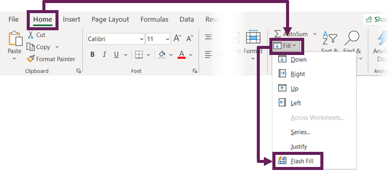
- Select the cells in the range to be filled with values (cells C2 to C11 in our example), click Home > Fill (dropdown) > Flash Fill.

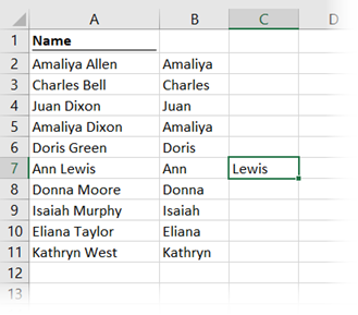
And we’re done. Both first name and last name have been separated into columns. I’ve shown the background and manual methods above; you can use either.
Note about Flash Fill
While Flash Fill in Excel is very good at identifying patterns, it will not always return the values you are expecting in more complex scenarios. There needs to be some logical pattern for it to find.
Flash Fill returns static values. If the source cells change, we need to re-run the process.
Flash Fill is also available in Data (tab) > Flash Fill
If Excel is unable to understand the pattern, it will return an error message.

Hopefully, you’ll agree that this future is any quick transformation we may want to make to the cells in Excel.
Split cells using Power Query
Another option for splitting multiple cells in Excel is to use Power Query. This has been natively available since Excel 2016. Prior to that, there was an add-in for Excel 2010 and 2013.
First, let’s load our cells into the Power Query editor.
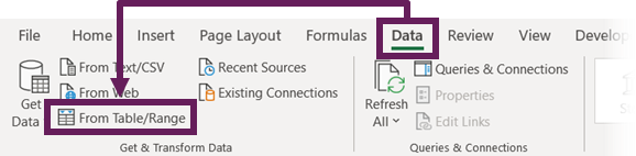
- Select any cell in the data set, then click Data (tab) > From Table/Range (or Data (tab) > From Sheet in newer versions of Excel) from the ribbon.

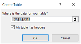
- If the selected cell is not part of an Excel table already, the Create Table box opens. Ensure the full range is selected, and my table has headers option is checked. Then click OK.

- The Power Query editor will open with all the data displayed.
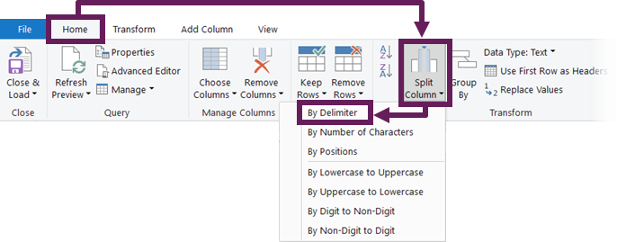
- From the Power Query ribbon select Home > Split Column (drop-down) > By Delimiter.

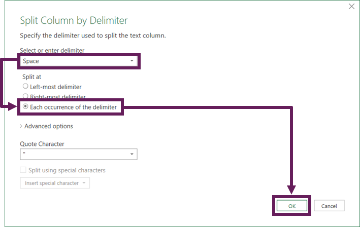
- Depending on the complexity of your text, there are lots of options to split the contents of a cell by different positions. For our scenario, the Space character and each occurrence of the delimiter are good options. Click OK.

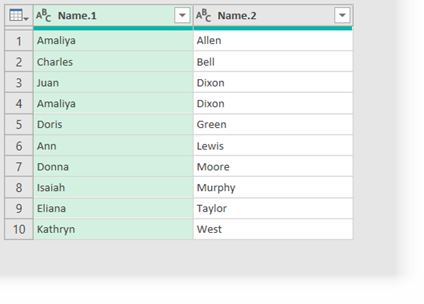
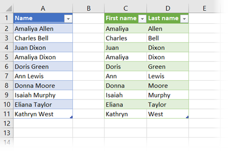
- In the data preview window, we now have the name split into two different columns.

- In the data preview window, Double click the header and change the headings to First and Last respectively.
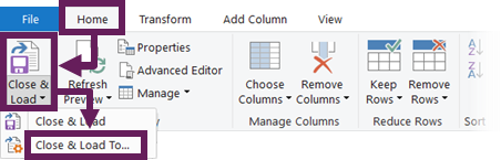
- Now we need to get the data back into Excel. Click Home > Close & Load (drop-down) > Close & Load To…

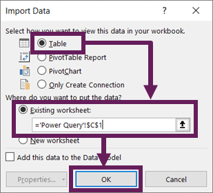
- From the Import Data dialog box, select Table and choose where to load the information back to. In the example, I have selected an existing sheet at cell C1. Click OK.

The transformed data will now be loaded back into the cells in Excel.
Note about Power Query
If our source cells change or more names are added, we can simply click Data (tab) > Refresh All, to refresh the output.
This method will change the source cells into an Excel table even if you don’t want it to.
If splitting by delimiters is not powerful enough, Power Query can transform more complex strings using the Column from Examples feature.
Power Query provides a lot of advanced tools to handle more complex data manipulation. If you’ve not used Power Query much, then check out my Introduction to Power Query series.
Split cells using Excel formulas
In answering the question of how to split a cell in Excel, our final option is to use standard Excel formulas. These give us the ability to split the contents of a cell using any rules we can program into our formulas. While formulas are very powerful, they also require our skill rather than using a point-and-click interface.
Useful Excel functions to split cells
The most useful functions to split multiple cells are:
LEFT
Returns the specified number of characters from the start of a text string.
Example:
=LEFT("Doris Green", 5)
Result: Doris
The second argument of 5 is telling the function to return the first 5 characters of the text “Doris Green”.
RIGHT
Returns the specified number of characters from the end of a text string.
Example:
=RIGHT("Kathryn West", 4)
Result: West
The second argument of 4 is telling the function to return the last 4 characters of the text “Kathryn West”.
MID
MID returns the characters from the middle of a text string, given a starting position and length.
Example:
=MID("Ann Lewis", 5, 3)
Result: Lew
The second argument represents the nth character to start from, and the last argument is the length of the string. From the text “Ann Lewis”, the 3 characters starting at position 5 are “Lew”.
LEN
Returns the number of characters in a text string.
Example:
=LEN("Amaliya Dixon")
Result: 13
There are 13 characters in the string (including spaces).
SEARCH
SEARCH returns the number of characters at which a specific character or text string is first found. SEARCH reads left to right and is not case sensitive.
Example:
=SEARCH(" ","Charles Bell",1)
Result: 8
The space character first appears in the 8th position of the string “Charles Bell”; therefore, the value returned is 8.
The last argument is optional; it provides the position to start searching from. If excluded, the count will start at the first character.
Note: FIND is the case-sensitive equivalent of the SEARCH function.
SUBSTITUTE
SUBSTITUTE replaces all existing instances of a text string with a new text string.
Example:
=SUBSTITUTE("Juan Dixon","Dix","Wils",1)
Result: Juan Wilson
The text string of Dix has been replaced with Wils. The last argument determines which instance to replace. In the formula above, it has replaced the 1st instance only. If we had excluded this argument, it would have replaced every instance.
Example scenario
Our scenario is reasonably simple, to split a cell into multiple columns we can use the LEFT, RIGHT, LEN and SEARCH functions. We can extract the first and last name as follows:
First name:
=LEFT(A2,SEARCH(" ",A2)-1)
- SEARCH finds the space character’s position, which for the first record in the example cells of “Amaliya Allen” is the 8th position.
- We do not want the space character included in the string, so we minus 1 from the result to give us a value of 7.
- LEFT then extracts the first 7 characters of the text string.
Last name:
=RIGHT(A2,LEN(A2)-SEARCH(" ",A2))
- LEN finds the length of the text string, which for “Amaliya Allen” is 13.
- SEARCH finds the position of the space character, which is 8.
- 13 minus 8 provides us with the number of characters after the first space.
- RIGHT is then used to extract the characters after the space.
With these two formulas, it gets us back to the same result as we’ve had before; first name in Column B and last name in Column C:
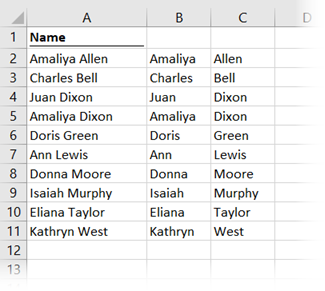
Notes about using formulas
Formulas are the only option in this post that are fully dynamic. If the original text changes, the formula result updates automatically too.
Depending on the complexity of the text string to be split, these formulas can become quite complex.
Conclusion
With these 4 techniques, you have learned how to split cells in Excel. Each option has added more and more power to deal with complexity. Which option you choose comes down to your specific scenario. Familiarize yourself with all the options, and then you’ll be able to make the best decisions.

About the author
Hey, I’m Mark, and I run Excel Off The Grid.
My parents tell me that at the age of 7 I declared I was going to become a qualified accountant. I was either psychic or had no imagination, as that is exactly what happened. However, it wasn’t until I was 35 that my journey really began.
In 2015, I started a new job, for which I was regularly working after 10pm. As a result, I rarely saw my children during the week. So, I started searching for the secrets to automating Excel. I discovered that by building a small number of simple tools, I could combine them together in different ways to automate nearly all my regular tasks. This meant I could work less hours (and I got pay raises!). Today, I teach these techniques to other professionals in our training program so they too can spend less time at work (and more time with their children and doing the things they love).
Do you need help adapting this post to your needs?
I’m guessing the examples in this post don’t exactly match your situation. We all use Excel differently, so it’s impossible to write a post that will meet everybody’s needs. By taking the time to understand the techniques and principles in this post (and elsewhere on this site), you should be able to adapt it to your needs.
But, if you’re still struggling you should:
- Read other blogs, or watch YouTube videos on the same topic. You will benefit much more by discovering your own solutions.
- Ask the ‘Excel Ninja’ in your office. It’s amazing what things other people know.
- Ask a question in a forum like Mr Excel, or the Microsoft Answers Community. Remember, the people on these forums are generally giving their time for free. So take care to craft your question, make sure it’s clear and concise. List all the things you’ve tried, and provide screenshots, code segments and example workbooks.
- Use Excel Rescue, who are my consultancy partner. They help by providing solutions to smaller Excel problems.
What next?
Don’t go yet, there is plenty more to learn on Excel Off The Grid. Check out the latest posts:
Splitting Cells in Excel refers to dividing its content into two or more separate cells. Splitting cells is often required when large datasets are imported in excel from external sources. In such cases, there is a need to create separate columns for similar data values.
For example, a journalist, Mr. D, wants to evaluate the number of awards won by the players of his country in an international sporting event. Further, he wants to present this data on a news channel in order to encourage the next generation to opt for a career in sports.
For this purpose, Mr. D has been given the following dataset:
- Column A lists the names of players, the countries they represent, and the games they are associated with.
- Column B displays the number of medals and trophies won by every player.
However, since all entries in column A are separated by a comma, it is difficult for Mr. D to comprehend the information. Moreover, the data is not presentable for the audience.
Hence, Mr. D wants to split the values of column A into separate columns in order to arrange the data neatly. This is where the splitting of cells property is applied.
The purpose of splitting excel cells is to organize, structure, and filter data to make it fit for analysis and decision-making. In addition, the splitting of cells helps to analyze every column independently.
To split cells in excel, the text to columns wizard is used, which consists of the following options:
- Delimited: It splits the excel cells based on a specified separator (delimiter) used in the source data file.
- Fixed width: It splits the excel cells based on the position at which the break line (vertical line) is inserted in the dataset. This property works well when all the substrings have a fixed length.
The text to columns wizard can be accessed either from the Data tab or the shortcut “Alt+A+E” (press one by one).
Table of contents
- How to Split a Cell in Excel?
- Example #1–Split by “Delimited” Option
- Example #2–Split by “Fixed Width” Option
- Frequently Asked Questions
- Recommended Articles
How to Split a Cell in Excel?
Let us consider some examples to understand the splitting of cells with the help of the Text to columns in excel is used to separate text in different columns based on some delimited or fixed width. This is done either by using a delimiter such as a comma, space or hyphen, or using fixed defined width to separate a text in the adjacent columns.read moretext to columnsText to columns in excel is used to separate text in different columns based on some delimited or fixed width. This is done either by using a delimiter such as a comma, space or hyphen, or using fixed defined width to separate a text in the adjacent columns.read more wizard.
You can download this Split a Cell Excel Template here – Split a Cell Excel Template
Example #1–Split by “Delimited” Option
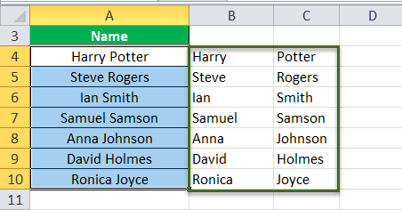
The following table shows the full names of seven people. We want to split the first and the last name into separate columns. Use the “delimited” option of the text to columns wizard.

The steps to split cells in excel with the help of the delimiter character are listed as follows:
- Select the cell range A3:A10, which is to be split. The same is shown in the following image.

- In the Data tab, click the “text to columns” option under the “data tools” group.

- The “convert text to columns wizard” dialog box appears, as shown in the following image.

- Choose the “delimited” option, which is selected by default. This option helps separate the data strings based on a particular delimiter character. Click “next.”
- Under “delimiters,” select the checkbox for space. Deselect the other delimiters (if selected), as shown in the following image. Click “next.”

- Under “destination,” specify the cell in which the output is required. Enter “$B$4” and click “finish.”
Note: If you proceed with the default cell address under “destination,” the output will replace the original dataset. To retain the initial data as is, select a cell to its right as the “destination.”

- The output is shown in the following image. The names of column A have been split into the first name (column B) and the last name (column C).
Note: The results of the “text to columns” property are static. This means that any change made to the source data is not reflected in the results. Hence, to include the changes, the whole process has to be repeated.


Example #2–Split by “Fixed Width” Option
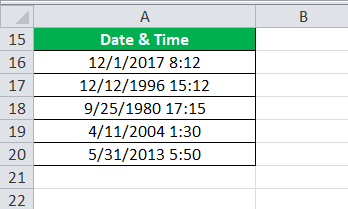
The following list shows the date and time of specific days. We want to split the date and time into separate columns. Use the “fixed width” option of the text to columns wizard.
Step 1: Select the range A16:A20, as shown in the following image. In the Data tab, click “text to columns” under the “data tools” group.

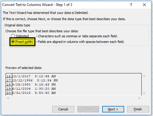
Step 2: The “convert text to columns wizard” dialog box appears. Select the option “fixed width,” as shown in the following image. Click “next.”
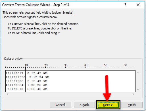
Step 3: Under “data preview,” place a break line (on the text) at the position where splitting is to be carried out.
Since we want to split the date and time, we insert the break line between these two data strings. Click “next.”
Note: To remove the break line, double-click on it.
Step 4: Under “column data format,” select date, as shown in the following image. In “destination,” enter the cell address where the results are required. Click “finish.”
Step 5: The output is shown in the following image. The data strings of column A have been split into the dates (column B) and the time (column C).

Frequently Asked Questions
1. What is the splitting of cells and how is it done in Excel?
When a cell is split, its components are divided into separate cells. Splitting is often done when there is a need to sort and re-arrange the existing data. Since the substrings of data are moved to new cells, splitting helps to analyze the resulting columns.
To split an excel cell, the text to columns feature is used. This separates the data of a cell, based on either the delimiter character or the fixed length of a substring.
The steps to split cell in excel are listed as follows:
a. Select the cells to be divided. In the Data tab, click “text to columns” under the “data tools” group.
b. Select the option “delimited” or “fixed width.” Click “next.”
c. If “delimited” is selected, enter the required separator in “delimiters.” If “fixed width” is selected, insert the break line at the desired position.
d. Select the “column data format” and specify the “destination.” Click “finish.”
The content of the selected cells is split into different excel columns.
2. How to split a cell’s content separated by commas into multiple cells of Excel?
Let us split column A which consists of data strings separated by a comma and space.
The entries in the range A1:A5 are listed as follows:
• Jack Adams, Chicago, USA, 2016
• Peter Smith, Houston, USA, 2019
• Ella Taylor, Glasgow, UK, 2018
• Lily Brown, Birmingham, UK, 2015
• Birdie Evans, Paris, France, 2020
The steps to split data into multiple cells using the “delimited” option are stated as follows:
a. In the Data tab, select the option “text to columns.” This is under the “data tools” group.
b. The “convert text to columns wizard” dialog box appears. Select “delimited” under “choose the file type that best describes your data.” Click “next.”
c. Select the checkboxes for both comma and space. Select the checkbox for “treat consecutive delimiters as one.” Click “next.”
d. Select “general” under the “column data format.” Enter “$B$1” under “destination.” Click “finish.”
Five separate columns (columns B to F) are created containing the first names, last names, cities, countries, and years respectively.
Note 1: Before the procedure begins, ensure that there are empty columns to the right of the destination cell. This prevents overwriting the source data.
Note 2: It is recommended to glance through the “data preview” before clicking “finish” in the last step. This ensures that the splitting of data is executed properly.
3. How to split cells in Excel automatically?
The flash fill feature helps to split cells automatically. When the user enters the split up text in a few cells one by one, Excel senses a pattern and fills the remaining cells.
Let us split the first and the last names of column A containing Jack Adams, Peter Smith, Ella Taylor, Lily Brown, and Birdie Evans (in the range A1:A5).
The steps of splitting excel cells with the help of flash fill are listed as follows:
a. In column B, enter the first name “Jack” in cell B1.
b. Enter “Peter” in the subsequent cell B2.
c. Excel detects a pattern and displays the first names for the remaining cells B3, B4, and B5. Press the “Enter” key.
Column B is filled with the first names (in the range B1:B5).
Note 1: Ensure that the first names in cells B1 and B2 are entered without the double quotation marks.
Note 2: Alternatively, after the first step (step a), click “flash fill” under the “data tools” group of the Data tab. This populates similar data in the remaining cells.
Recommended Articles
This has been a guide to splitting a cell in Excel. Here we discuss how to split a cell in Excel by using the text to columns wizard (delimited and fixed-width method) along with Excel examples and downloadable Excel templates. You may also look at these useful functions of Excel–
- Convert Excel Text to Numbers
- Combine Cells in Excel
- Merge Cells in Excel
- Unmerge Cells in Excel
- Change Case in Excel
You may need to split a value in your cell into two or more columns by space, character, or another delimiter. This can be done easily with a few clicks. On the other hand, some users need to split cells into rows. Although Excel does not have this functionality out of the box, you can use a few functions to do the job. Read on to learn all the options available for splitting cells in Excel.
You can split cells in Excel with the following options:
- Using a native functionality
- Using a combination of Excel functions
- Power Query
- Visual Basic for Applications (VBA)
For this article, we have decided to group the use cases not by option, but by the expected outcome. So, we’ll cover two epic tasks: split cells to columns and split cells to rows. Each of these tasks will include the options to split by different delimiters and other specific requirements.
For the examples below, we imported data from different sources such as Airtable, Google Sheets, and BigQuery with Coupler.io. It’s a powerful solution for getting data to Excel from multiple apps and web APIs without coding. The main benefit is that you can synchronize your workbook with your data source on a custom schedule!

Check out the Microsoft Excel integrations available.
Let’s check out each option so you can choose the one that works best for your task.
How to split one cell into two cells in Excel
We’ll warm up with a simple example of splitting a full name, Margeaux Kuhnke, into first and last name cells. Go to the Data ribbon and click Text to Columns.
A wizard will open, where you’ll need to perform three steps:
- Choose the way to split your data: by a delimiter or by a fixed width
- Set delimiters or field width depending on which splitting method you chose before. In our example, we need to split a cell by space as a delimiter.

- Select the date format and destination cell. If you want to keep the source value, choose a different cell as a destination.

Once you click “Finish“, your cell will be split into the number of cells depending on the number of delimiters in your source value. In our example, we had one delimiter, so the cell was split into two cells.

Split text in Excel cell into multiple cells by space
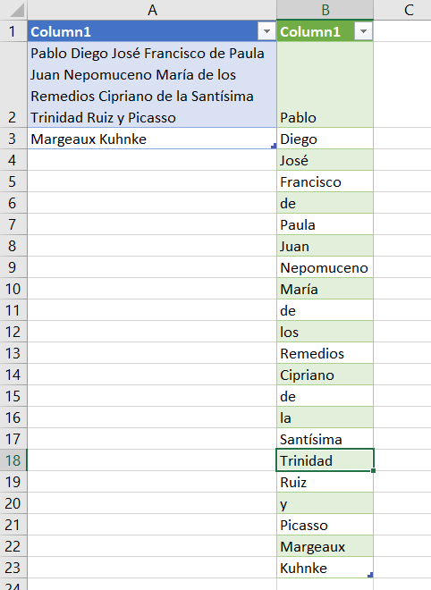
If a full name in a cell consists of three or more names, the number of split cells will be greater. For example, let’s split Pablo Picasso’s full name using space as a delimiter:
Pablo Diego José Francisco de Paula Juan Nepomuceno María de los Remedios Cipriano de la Santísima Trinidad Ruiz y Picasso

The outcome is that we’ve split the text in the Excel cell into multiple cells (20!) by spaces!

Excel split cells by character
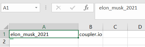
Splitting cells by character may be useful if you need to separate, for example, username and domain name in email addresses. Let’s say we have a fictional user with the following email address:
elon_musk_2021@coupler.io
In this case, the delimiter is a character: @. So, we need to specify this.

There you go!
Excel split data in cell by line break
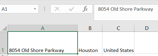
What if your cell contains a few lines like an address, and you want each line in its own cell?
8054 Old Shore Parkway
Houston
United States
To split this string, you need to specify the line break as a delimiter. To do this, choose Other as a delimiter and press Ctrl + J.

Here is the result:
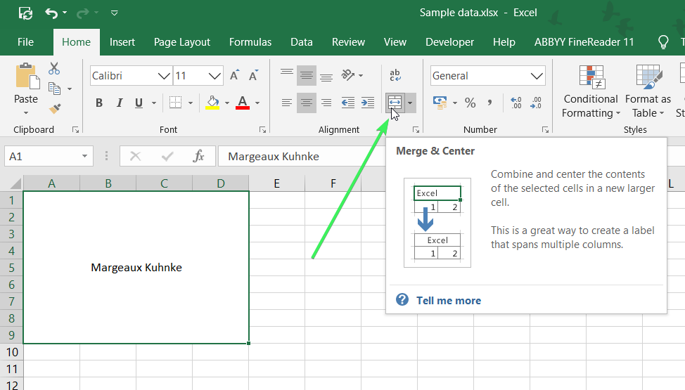
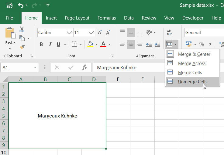
How to split merged cells in Excel
Splitting merged cells is a slightly different concept, since it does not affect the content of the cells. You can do this easily using the Merge & Center button.
Select the merged cells, open the drop-down options and click Unmerge Cells.
Split cells into rows in Excel
Unfortunately, there is no single button or function to split a cell into rows or to split cells vertically in Excel. Nevertheless, you can do this with the help of Excel functions or Power Query. But first, check out this easy method for splitting cells into rows.
Split Excel cell into two rows easily
You’ll need to take two steps:
- Split your cell using the Text to Columns button as we explained before.

- Copy the resulting cells and paste them using Paste special => Transpose.

This is the simplest way to split cells to rows in Excel, but it’s manual. Let’s discover some options to automate the flow.
Split cells vertically in Excel with formulas
Let’s take the previous example of splitting a full name: Margeaux Kuhnke.
We’ll need two formulas for each row:
- First
= LEFT(cell, FIND(" ",cell) - 1)
This formula extracts a string before the specified delimiter: FIND(" ",cell).
2. Second
= RIGHT(cell, LEN(cell) - FIND(" ",cell))
This formula extracts a string after the specified delimiter.
If you have two or more delimiters, both formulas will only work with the first delimiter, like this:

If for some reason you need to split a cell by a second or third delimiter, you need to update the FIND formula, keeping the following logic in mind:
=FIND("delimiter",cell,starting_position)starting_position– specify the starting position (character) to skip the unnecessary delimiters.
In our example, to split the cell by the second delimiter, the formulas will look like this:
=LEFT(A1,FIND(" ",A1,10)-1)
=RIGHT(A1, LEN(A1) - FIND( " ",A1,10) )

Split cells in Excel into multiple rows
Unfortunately, these formulas do not apply to the “Pablo Picasso” case, where the number of delimiters is 19! For such cases, the following formula works better:
=FILTERXML("<t><s>" &SUBSTITUTE($cell," ", "</s><s>") & "</s></t>", "//s")This converts cell contents into an XML string and then extracts data from it. This formula should be executed as an array formula; that is, you need to select the cell to split into and press Ctrl+Shift+Enter. Here is how it works with the Pablo Picasso’s full name:
=FILTERXML("<t><s>" &SUBSTITUTE($A$1," ", "</s><s>") & "</s></t>", "//s")

You can also use this formula to extract specific pieces of your string by specifying them as follows:
=FILTERXML("<t><s>" &SUBSTITUTE($cell," ", "</s><s>") & "</s></t>", "//s"[number_of_piece])For example, to extract the third name from the Picasso’s full name, we update our formula as follows:
=FILTERXML("<t><s>" &SUBSTITUTE($A$1," ", "</s><s>") & "</s></t>", "//s[3]")

How to split cells to rows or columns in Excel dynamically without formulas
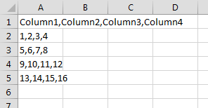
If you don’t want to mess with formulas for your splitting tasks, but you want to have a dynamic approach, check out the Power Query method. Let’s check it out for our Pablo Picasso example.
- Go to Data => From Table.
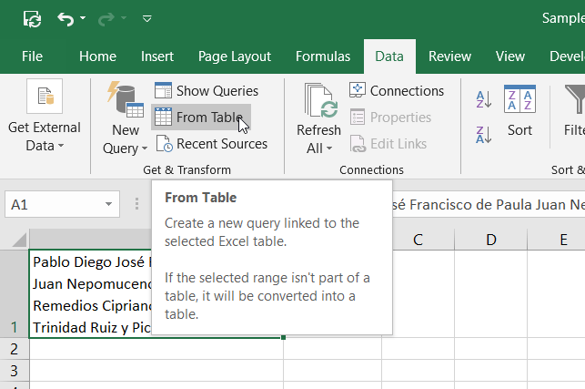
- Select the cell with your data and click “OK“.

- After that, the Power Query Editor will open. Then select Split Column => By Delimiter.

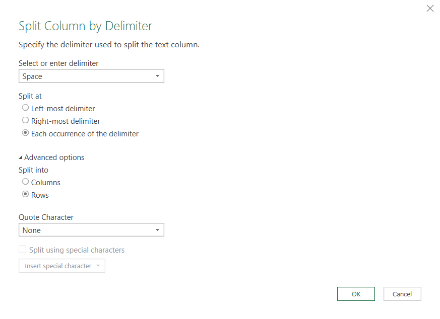
- Select your delimiter, click “Advanced options“, choose Split into Rows, and select “None” as a Quote Character.
- The data will be split into rows. Now you need to save and load it. For this, click:
- “Close & Load” to load data in a new worksheet.
- “Close & Load To…” to specify a custom destination for your data.

There you go!

Now, every value added to the A column will be split into rows by space. Just click refresh to see the split values.
See, with Power Query you can also split cells into columns by different delimiters.
Bonus: How to split cells diagonally in Excel
By diagonal split, users usually mean crossing a cell with a diagonal border like this:
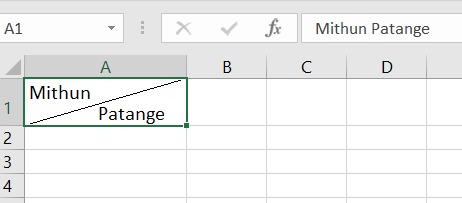
This does not split a cell into columns or rows, but makes a visual split of two values in the cell. Here is how you can do this.
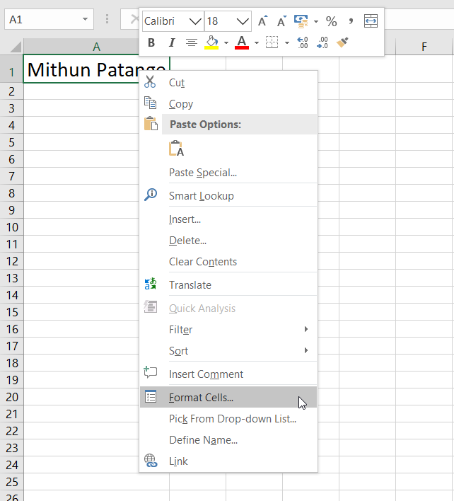
- Right-click on the cell you want to split diagonally and select Format Cells…
- In the open dialog window, go to the Border tab and click the diagonal border.
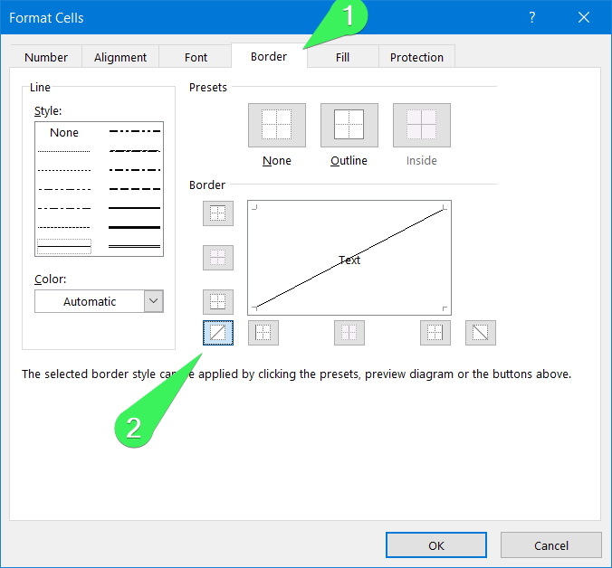
- Click OK and you will see a line splitting the selected cell diagonally. But this is not quite how we want it to look.

- To fix this, we need to assign the Superscript font effect to one value in the cell, and Subscript to the other value. Select one word – in our case, this is “Mithun“. Then go to the Home tab and click the Font Settings – a small arrow at the bottom-right corner of the Font section.
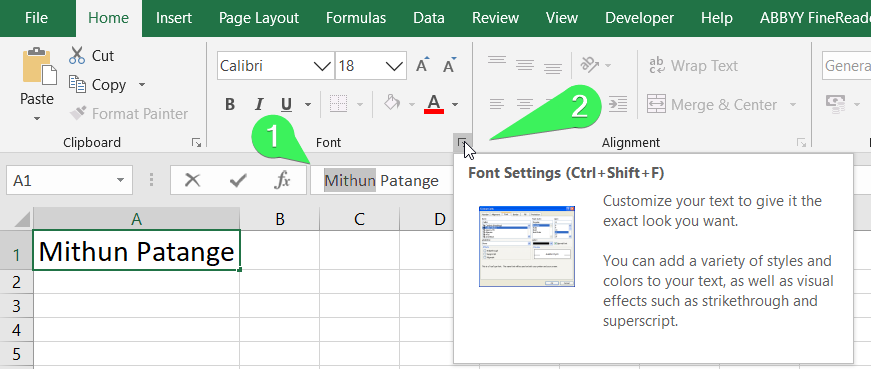
- In the dialog box, check the Superscript font effect and click OK.

- Here is how it looks now

- Now, do the same with the second value using the Subscript option.

- And there you go!
Are there other options to split cells in Excel?
In Excel, there is no dedicated function for splitting data, like SPLIT in Google Sheets. However, using Excel VBA, you can build a custom VBA function to solve your specific splitting tasks. This requires knowledge of Microsoft Visual Basic for Applications.
However, for most cases, the options previously described will do the job. Good luck with splitting your data!
-

A content manager at Coupler.io whose key responsibility is to ensure that the readers love our content on the blog. With 5 years of experience as a wordsmith in SaaS, I know how to make texts resonate with readers’ queries✍🏼

Back to Blog
Focus on your business
goals while we take care of your data!
Try Coupler.io
The easiest way on how to split Cells in Excel or split Columns in Excel, is to select the column you want to split. Next go to the Data ribbon and hover to the Data Tools group. Next Select Text to Columns and proceed according to the instructions.
The above works for simple splits on delimiters such as Commas, Semicolons, Tabs etc. However, for Non-Standard patterns such as Capital letters, specific word you might need to revert to more elaborate solutions such using VBA String functions or the VBA Regex. Read on to learn more.
Splitting Cells using Text to Columns
A Delimiter is a sequence of 1 or more characters to separate columns within a Text String. An example of a Delimiter is the Comma in the following Text String Columns1,Column2 which separates the String Column1 from Column2. Popular Delimiters often used are: Commas (,), Semicolons (;), Dots (.), Tabs (t), Spaces (s). A Delimiter can be just as well any Sequence of Characters.
How to Split Cells in Excel using Text to Columns
The most obvious choice when wanting to Split Cells in Excel is to use the DATA Ribbon Text to Columns feature.
Select the Column
Select the Column with Cells you want to Split in Excel:
Select first column and proceed to Text to Columns
Select the entire first column where all your data should be located. Next click on the Text to Columns button in the DATA ribbon tab:
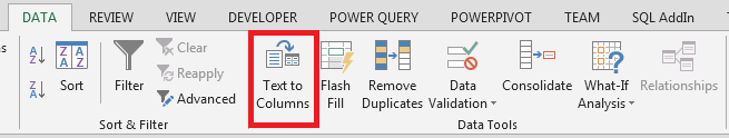
Proceed according to Wizard instructions
This is the hard part. Text to Columns need additional information on the delimiter and format of your columns.
Delimited or Fixed width?
Delimiters are any specific Sequence of Characters (like a comma or semicolon). Fixed Width means that each column in the Cell is separated by a Fixed Width of Whitespace Characters. In this case we select Delimited. Next click Next to proceed.
Select delimiter
Assuming your columns are separated with a specific Delimiter you need to provide this delimiter in the Wizard. Look at the Data preview to make sure your columns will be separated correctly. When finished proceed with Next
Format your columns (optional)
The last step is to format your columns if needed. If your columns represent Dates or you want to pull a column containing numbers/dates as text instead – be sure to format it appropriately. Usually, however, you are fine with hitting Finish:
The Resulting Split Columns
If you have proceeded according to the steps above you should have a neatly formatted spreadsheet like the one below.
Splitting Cells using Formulas
Another way of how to Split Cells in Excel is using the LEFT, RIGHT and LEN functions. See examples below:
Splitting against a Delimiter:
'Cell A1
Hello;There
The formula:
'To get "Hello"
=LEFT(A1;FIND(";")-1)

'To get "There"
=RIGHT(A1;LEN(A1)-FIND(";"))
Split Cells on Patterns
Sometimes instead of Delimiters you want to Split your Excel Cells on Patterns that are dynamic and may be different for each cell in a certain column. Fortunately Excel supports Regular Expressions, which allow you to Define Patterns on which your Cells are to be Split.
Let us first introduce my often used GetRegex UDF function:
'str - the original string. reg - the Regex pattern. index - the index of the capture if more than 1.
Public Function GetRegex(str As String, reg As String, Optional index As Integer) As String
    On Error Resume Next
    Set regex = CreateObject("VBScript.RegExp")
    regex.Pattern = reg
    regex.Global = True
    If index < 0 Then index = 0
    If regex.test(str) Then
        Set matches = regex.Execute(str)
        GetRegex = matches(index).SubMatches(0)
        Exit Function
    End If
    GetRegex = ""
End Function
To install it – open your DEVELOPER Excel Tab, click Visual Basic and add the code above to any new VBA Module.
If you are not familiar with Regular Expressions read the VBA Regex Tutorial.
What does this UDF function do? It extracts any text that matches a certain pattern. Let’s see it in action:
Example 1: Splitting Cells on Capital Letters
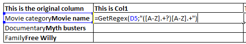
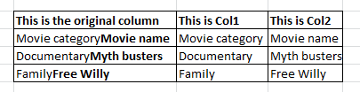
Let us take a common example where we have 1 Column of Cells that have 2 merged Columns inside. We want to split them on the second capital letter:
Now splitting this on the second capital letter using the FIND, LEFT, RIGHT and LEN functions will be a nightmare.
Let’s decipher the regular expression now:
| Pattern | Description |
|---|---|
| [A-Z].+? | This will catch all words and whitespaces starting with a Capital letter the ? sign means that this is a non-greedy regular expression |
| ([A-Z].+?) | The () brackets will capture inside any pattern matching this regular expression |
| ([A-Z].+?)[A-Z].+ | The final regex this will capture only the first words and whitespaces starting with a Capital letter. Notice that the capture will end at the next Capital letter |
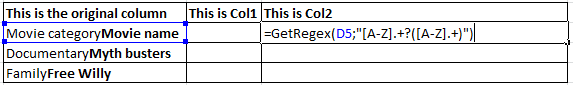
Now for the second column:
Great right? Now just drag the formula across the rows – and you are done!
Example 2: Splitting Cells on Whitespaces
A simple example – let us Split an Excel Cell on a Variable number of Whitespace characters. Let us say the Words in our String can have 1 or more Spaces in between.
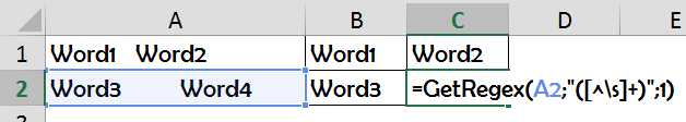
The Formula for the above is:
=GetRegex(A1;"s*?([^s]+)s*?";0)
Again let us break it down:
| Pattern | Description |
|---|---|
| [^s] | This specifies a non-whitespace character |
| [^s]+ | This specifies at least 1 non-whitespace character |
| ([^s]+) | The () brackets will capture inside any pattern matching this regular expression – hence all sequences of non-whitespace characters |
Split Excel Function
If you just need an Excel Split function and you can introduce the following UDF Function (copy to VBA Module):
Public Function SplitFunction(str As String, delimiter As String, index As Long) As String
    SplitFunction = Split(str, delimiter)(index)
End Function
It uses the VBA Split function which is available in VBA only.
Parameters
str
A String.
delimiter
The delimiter on which the Split operation is to be done.
index
The index of the substring resulting from the Split.
How to use the Excel Split Function
The Function will be available as an Excel Function:
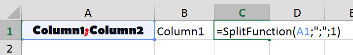
The above Formula looks like this (return second substring from Split):
=SplitFunction(A1;";";1)