
Select cell contents in Excel
In Excel, you can select cell contents of one or more cells, rows and columns.

Note: If a worksheet has been protected, you might not be able to select cells or their contents on a worksheet.
Select one or more cells
-
Click on a cell to select it. Or use the keyboard to navigate to it and select it.
-
To select a range, select a cell, then with the left mouse button pressed, drag over the other cells.
Or use the Shift + arrow keys to select the range.
-
To select non-adjacent cells and cell ranges, hold Ctrl and select the cells.
Select one or more rows and columns
-
Select the letter at the top to select the entire column. Or click on any cell in the column and then press Ctrl + Space.
-
Select the row number to select the entire row. Or click on any cell in the row and then press Shift + Space.
-
To select non-adjacent rows or columns, hold Ctrl and select the row or column numbers.
Select table, list or worksheet
-
To select a list or table, select a cell in the list or table and press Ctrl + A.
-
To select the entire worksheet, click the Select All button at the top left corner.


Note: In some cases, selecting a cell may result in the selection of multiple adjacent cells as well. For tips on how to resolve this issue, see this post How do I stop Excel from highlighting two cells at once? in the community.
|
To select |
Do this |
|---|---|
|
A single cell |
Click the cell, or press the arrow keys to move to the cell. |
|
A range of cells |
Click the first cell in the range, and then drag to the last cell, or hold down SHIFT while you press the arrow keys to extend the selection. You can also select the first cell in the range, and then press F8 to extend the selection by using the arrow keys. To stop extending the selection, press F8 again. |
|
A large range of cells |
Click the first cell in the range, and then hold down SHIFT while you click the last cell in the range. You can scroll to make the last cell visible. |
|
All cells on a worksheet |
Click the Select All button.
To select the entire worksheet, you can also press CTRL+A. Note: If the worksheet contains data, CTRL+A selects the current region. Pressing CTRL+A a second time selects the entire worksheet. |
|
Nonadjacent cells or cell ranges |
Select the first cell or range of cells, and then hold down CTRL while you select the other cells or ranges. You can also select the first cell or range of cells, and then press SHIFT+F8 to add another nonadjacent cell or range to the selection. To stop adding cells or ranges to the selection, press SHIFT+F8 again. Note: You cannot cancel the selection of a cell or range of cells in a nonadjacent selection without canceling the entire selection. |
|
An entire row or column |
Click the row or column heading.
1. Row heading 2. Column heading You can also select cells in a row or column by selecting the first cell and then pressing CTRL+SHIFT+ARROW key (RIGHT ARROW or LEFT ARROW for rows, UP ARROW or DOWN ARROW for columns). Note: If the row or column contains data, CTRL+SHIFT+ARROW key selects the row or column to the last used cell. Pressing CTRL+SHIFT+ARROW key a second time selects the entire row or column. |
|
Adjacent rows or columns |
Drag across the row or column headings. Or select the first row or column; then hold down SHIFT while you select the last row or column. |
|
Nonadjacent rows or columns |
Click the column or row heading of the first row or column in your selection; then hold down CTRL while you click the column or row headings of other rows or columns that you want to add to the selection. |
|
The first or last cell in a row or column |
Select a cell in the row or column, and then press CTRL+ARROW key (RIGHT ARROW or LEFT ARROW for rows, UP ARROW or DOWN ARROW for columns). |
|
The first or last cell on a worksheet or in a Microsoft Office Excel table |
Press CTRL+HOME to select the first cell on the worksheet or in an Excel list. Press CTRL+END to select the last cell on the worksheet or in an Excel list that contains data or formatting. |
|
Cells to the last used cell on the worksheet (lower-right corner) |
Select the first cell, and then press CTRL+SHIFT+END to extend the selection of cells to the last used cell on the worksheet (lower-right corner). |
|
Cells to the beginning of the worksheet |
Select the first cell, and then press CTRL+SHIFT+HOME to extend the selection of cells to the beginning of the worksheet. |
|
More or fewer cells than the active selection |
Hold down SHIFT while you click the last cell that you want to include in the new selection. The rectangular range between the active cell and the cell that you click becomes the new selection. |
Need more help?
You can always ask an expert in the Excel Tech Community or get support in the Answers community.
See Also
Select specific cells or ranges
Add or remove table rows and columns in an Excel table
Move or copy rows and columns
Transpose (rotate) data from rows to columns or vice versa
Freeze panes to lock rows and columns
Lock or unlock specific areas of a protected worksheet
Need more help?
Working with Excel means working with cells and ranges in the rows and columns in it.
And if you work with large datasets, selecting entire rows and columns is quite a common task.
Just like with most things in Excel, there is more than one way to select a column or row in Excel.
In this tutorial, I will show you how to select a column or row using a simple shortcut, as well as some other easy methods.
I will also show you how to do this when you’re working with an Excel table or Pivot Table.
So let’s get started!
Select Entire Column/Row Using Keyboard Shortcut
Let’s start with the keyboard shortcut.
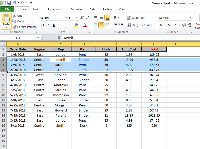
Suppose you have a dataset as shown below and you want to select an entire column (say column C).

The first thing to do is select any cell in Column C.
Once you have any cell in column C selected, use the below keyboard shortcut:
CONTROL + SPACE
Hold the Control key and then press the spacebar key on your keyboard
In case you’re using Excel on Mac, use COMMAND + SPACE
The above shortcut would instantly select the entire column (as you will see it gets highlighted in gray – indicating that it’s selected)

You can use the same shortcut to select multiple contiguous columns as well. For example, suppose you want to select both columns C and D.
To do this, select two adjacent cells (one in column C and one in Column D) and then use the same keyboard shortcut.
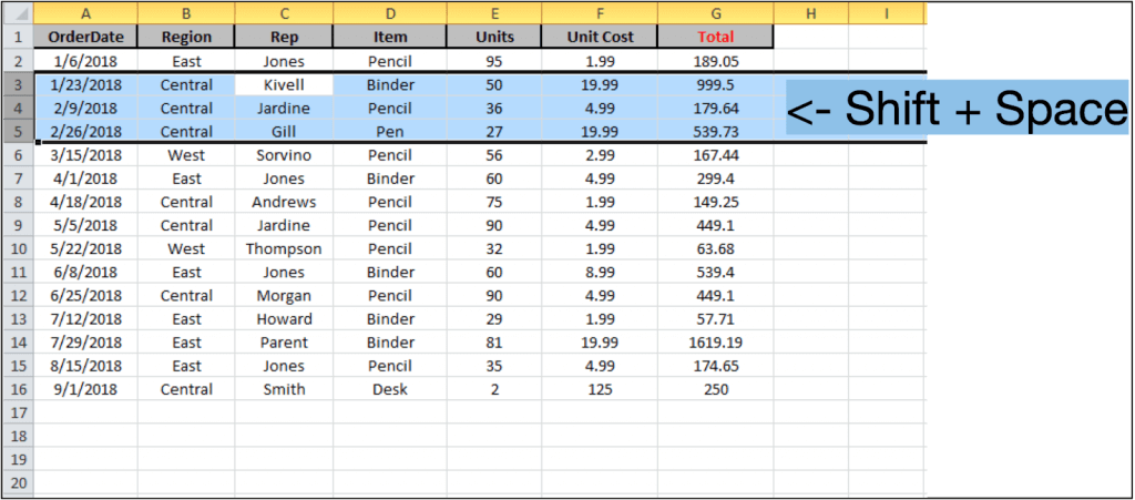
Selecting the Entire Row
If you want to select the entire row, select any cell in the row that you want to be selected and then use the below keyboard shortcut
SHIFT + SPACE
Hold the Shift key and then press the Spacebar key.
You will again see that it gets selected and highlighted in gray.

In case you want to select multiple contiguous rows, select multiple adjacent cells in the same column and then use the keyboard shortcut.
Also read: Select Every Other Row in Excel
Select Entire Column (or Multiple Columns) Using Mouse
I have a feeling you may already know this method, but let me cover it anyway (it will be short).
Select One Column (or Row)
If you want to select an entire column (say column D), hover the cursor over the column headers (where it says D). You will notice that the cursor changes to a black downward-pointing arrow.
Now, click the left mouse key.
Doing this will select the entire column D.

Similarly, if you want to select the entire row, click on the row number (in the row header on the left)
Select Multiple Contiguous Columns (or Rows)
Suppose you want to select multiple columns that are next to each other (say column D, E, and F)
Follow the below steps to do this:
- Place the cursor on the left most column header of column D
- Press the left mouse key and keep it pressed
- With the left key pressed, drag the mouse to also cover column E and F
The above steps would automatically select all the columns in between the first and the last selected column.

And the same way, you can also select multiple contiguous rows.
Select Multiple Non-Contiguous Columns (or Rows)
This is the most common scenario where you need to select multiple columns that are not next to each other (say column D, and F).
Below are the steps to do this:
- Place the cursor at the column heading of one of the columns (say column D in this case)
- Click the mouse left key to select the column
- Press and hold the Control key
- With the Control key pressed, select all the other columns you want to select

You can do the same with rows as well.
Select Entire Column (or Multiple Columns) Using Name Box
Use this method when you want to:
- Select a far-off row or column
- Select multiple contiguous or non-contiguos rows/columns
Name box is a small box that is left of the formula bar.

While the main purpose of the Name Box is to quickly name a cell or range of cells, you can also use it to quickly select any column (or row).
For example, if you want to select the entire column D, enter the following in the name box and hit enter:
D:D
Similarly, if you want to select multiple columns (say D, E, and F), enter the following in the name box:
D:F
And that’s not it!
If you want to select multiple columns that are not adjacent, say D, H, and I, you can enter the below:
D:D,H:H,I:I
When I used to work as a financial analyst years ago, I found this trick extremely useful. It allowed me to quickly select columns and format them at once, or delete/hide these columns in one go.
The Named Range Trick
Let me also show you another wonderful trick.
Suppose you’re working in a workbook where you may often have a need to select far-off columns (say column B, D, and G).
Instead of doing it one by one or entering it manually in the Name Box, here is what you can do – create a named range that refers to the columns you want to select.
Once created, you can simply enter the named range name in the Name box (or select it from the drop-down)
Below are the steps to create a named range for specific columns:
- Select the columns for which you want to create the named range (hold the Control key and then select the columns one-by-one)
- Enter the name you want to give to the selection in the Name Box (no spaces allowed in the name). In this example, I will use the name SalesData

- Hit Enter
Once this is done, you have created a named range in Excel that now refers to the columns you selected (B, D, and G in my example).
And now it’s time for magic.
If you want to quickly select the columns B, D, and G, just enter the name in the Name box and hit enter (or click on the small drop-down icon at the end of the name box and select the name from the list).

Voila, all the columns would be selected.

This technique is useful if you may have a need to select the same columns multiple times in the same sheet.
You can use this technique to select rows as well as different ranges. For example, if you want to select two separate ranges in Excel, just follow the same steps (instead of selected columns, select the ranges and give them a name).
Select Column in an Excel Table
When working with Excel Tables, you may sometimes have a need to select an entire row or column in the table.
This means that you don’t want to select the entire column in the worksheet, but the entire column of the table.
Here is the trick to do this:
- Place the cursor on the header of the Excel table (note this is the header of the column in the Excel table, not the one that displays the column letter)
- You will notice that the cursor would chnage into a downward pointing black arrow

- Click the left mouse key
The above steps would select the entire column in the Excel Table (and not the full column).
And if you want to select multiple columns, hold the Control key and repeat the process for all the columns you want to select.
Also read: AutoSum in Excel (Shortcut)
Select Column in an Pivot Table
Just like the Excel table, you can also quickly select an entire row or column in a Pivot Table.
Suppose you have a Pivot Table as shown below and you want to select the Sales columns,
Below are the steps to do this:
- Place the cursor on the header of the Pivot table header that you want to select
- You will notice that the cursor would chnage into a downward pointing black arrow

- Click the left mouse key
These steps would select the Sales column. Similarly, if you want to select multiple columns, hold the Control key and then make the selection.
So these are some of the common ways you can use to select an entire column or an entire row in Excel.
I hope you found this tutorial useful!
Other Excel tutorials you may also like:
- Flip Data in Excel | Reverse Order of Data in Column/Row
- How to Lock Row Height & Column Width in Excel (Easy Trick)
- How to Delete All Hidden Rows and Columns in Excel
- 7 Easy Ways to Select Multiple Cells in Excel
- How to Insert Multiple Rows in Excel
- How to Copy and Paste Column in Excel? 3 Easy Ways!
- How to Multiply a Column by a Number in Excel
- Select Till End of Data in a Column in Excel (Shortcuts)
- How to Group Columns in Excel?
When you are working with large amounts of data in spreadsheets, you need all the tips and tricks you can get to quickly access your required data.
Oftentimes you might need to work with selected rows in bulk.
For example, you might need to delete rows containing a specific text, or maybe format them a certain way.
In all these cases, if you are to work with them in one single go, you will need to first select these rows all at the same time. Unfortunately, selecting rows with specific text in Excel can be quite a tricky affair.
In this tutorial we will show you two ways in which you can select rows with specific text in Excel:
- Using VBA
- Using Data Filters
The first method is quick and easy, but involves a little bit of coding.
If you’re not comfortable with coding, you can opt for the second method.
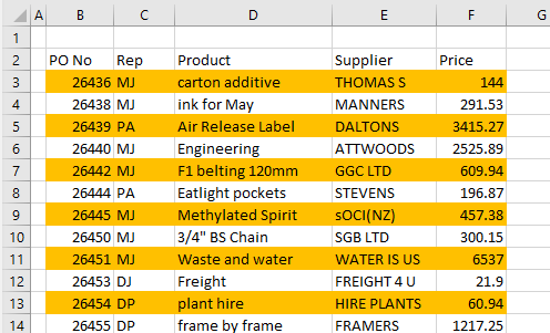
To demonstrate the two methods in this tutorial, we are going to use the following data:

Given the above data, let us say you want to find and select all the rows that contain the word “King” in them.
Here are two ways to tackle this problem.
Using VBA to Select Rows with Specific Text in Excel
This method involves coding in VBA.
We have already prepared the code that you need to use, so all you need to do is just navigate to the Developer window, copy-paste the code, select the data that you want to work on and run the code.
To use this code, you need to first select the data where you want to select rows with specific text and then run this code.
The following code will help you select rows with specific text in Excel.
'This code is developed by Steve from SpreadsheetPlanet.com
 Sub select_rows_with_given_string()
 Dim Rng As Range
 Dim myCell As Object
 Dim myUnion As Range
 Set Rng = Selection
 searchString = InputBox("Please Enter the Search String")
 For Each myCell In Rng
 If InStr(myCell.Text, searchString) Then
      If Not myUnion Is Nothing Then
          Set myUnion = Union(myUnion, myCell.EntireRow)
      Else
          Set myUnion = myCell.EntireRow
      End If
 End If
 Next
 If myUnion Is Nothing Then
     MsgBox "The text was not found in the selection"
 Else
     myUnion.Select
 End If
 End Sub
The above macro loops through each cell in a range and selects only the rows that contain the text “King”.
Note that the above code is case sensitive. In case you look for the word ‘king’, it will not be able to find it and show you a message box letting you know that it couldn’t find the specified text.
To enter the above code, copy it and paste it in your developer window.
Here’s how to copy and run this code:
- From the Developer tab, select Visual Basic.

- Once your VBA window opens, you will see all your files and folders in the Project Explorer on the left side. If you don’t see the Project Explorer, click on View->Project Explorer.

- Make sure ‘ThisWorkbook’ is selected under the VBA project with the same name as your Excel workbook.
- Click Insert->Module. A new module window should open up.

- Now you can start coding. Copy the above code script and paste into the module code window.

- Close the VBA window.
Your macro is now ready to use.
Note: If you don’t see the Developer ribbon, from the File menu, go to Options. Select Customize Ribbon and check the Developer option from Main Tabs. Finally, Click OK.
Now that we have copied the code in it’s rightful place, we need to run the code.
To run your macro, do the following:
- Select the range of cells that you want to work with.
- Select the Developer tab.
- Click on the Macros button (under the Code group).

- This will open the Macro Window, where you will find the names of all the macros that you have created so far.

- Select the macro (or module) named ‘select_rows_with_given_string’.
- Click Run.
- You will get an input box asking you to enter your search string.

- Type in the text you want to search for. In our example, we are looking to select all rows with the word ‘King’ in it. So we type ‘King’.
- Click OK.
- All the rows containing your search string should now be selected.

Now that your required rows are selected you can go ahead and perform whatever actions you need to with them.
You can also use this script and tweak it to suit your own requirements.
Explanation of the Code
So how did this code work?
In the above code we used the InputBox function to obtain the search string input from the user.
We then used a For-each loop to cycle through each cell in the given range (Rng). If a cell contains the given search string, we add the entire row of that cell to myUnion (a Range variable containing the range of all rows that we want to select).
To find out if a cell contains the given search string, we used the InStr function. Finally we used the command ‘myUnion.Select’ to select all the rows that have been added to myUnion.
In this way, the code selects all rows that contain the search string provided by the user.
Also read: How to Rearrange Rows In Excel
Using Filters to Select Rows with Specific Text in Excel
The VBA method is actually the best way to select rows with specific text in Excel.
However, if the idea of coding or using VBA intimidates you, then there’s an alternative way to get the job done.
This involves using Excel’s handy Filters feature. This feature lets you filter out rows that match a given criterion.
So you can easily use it to see which rows contain your specified text. It will filter out all other rows and show you only the matching ones.
So, you get all your required rows one below the other.
This makes it easy for you to select all the filtered rows in one go and perform subsequent actions on them.
Here are the steps that you need to follow if you want to use filters to select rows with specific text:
- Click on the header of any column in the range you want to work on.
- Click on the Data tab and select the Filter button (You’ll find it under the ‘Sort & Filter’ group.

- You should now see a small arrow button on every cell of the header row.

- These buttons are meant to help you filter your cells. You can click on any arrow to choose a filter for the corresponding column.
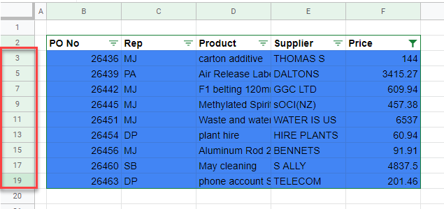
- In this example, we want to search for titles in the ‘Books’ column. So click on the arrow next to the ‘Books’ header.

- This will display a drop-down with different filtering options. In the input box under ‘Text Filters’, type your search string. Since we are looking for the word ‘King’, we will type that into the input box.

- Click OK.
- You should now be able to see only those rows that contain the word ‘King’ in the Books column.

- You can now select the row headers of all the displayed rows altogether. This will cause only the visible rows to get selected. The hidden rows (which do not contain the word ‘King’) will not be selected.

Now that your required rows are selected, you can go ahead and copy them, delete them or perform whatever tasks you need to with them.
One thing that I like about this method is that it allows you to apply multiple conditions at the same time and then allow you to select the records.
For example, if I want to select all the rows where the book name has the word ‘King’ and the book availability status is Yes, then I can do that. All I need to do is apply two separate filters and then select the rows that remain.
In this tutorial we showed you two tricks to select rows with specific text in Excel.
I hope this was helpful and easy for you to apply.
Some other Excel tutorials you may also like:
- How to Add a Total Row in Excel Table
- How to Select Multiple Rows in Excel
- How to Hide Rows based on Cell Value in Excel
- How to Delete Filtered Rows in Excel (with and without VBA)
- How to Highlight Every Other Row in Excel (Conditional Formatting & VBA)
- How to Unhide All Rows in Excel with VBA
- How to Set a Row to Print on Every Page in Excel
- How to Select Every Other Cell in Excel (Or Every Nth Cell)
- How to Move Row to Another Sheet Based On Cell Value in Excel?
- How to Delete Hidden Rows or Columns in Excel? 2 Easy Ways!
While working on Excel spreadsheets, some of the tasks are used commonly, such as selection, grouping, sorting out data, and so on. Talking about the selection task, you will tenderly need to use it while working with multiple formulas or other functions. You may have to use it to select one or more rows. Well, these are some of the general examples of selection. You might be needing to select data in every other row in Excel and for this, you can use the best ways mentioned below.
How to Select Every Other Row in Excel?
Here we have some useful tricks that you can follow to describe the possibility of how to select every other row in Excel. Let’s find it out:
- With CTRL and Mouse Click
- Using Conditional Formatting
- Format Data as a Table
- Go To Special hack
- VBA (Automation)
Using CTRL and Mouse Click to Select Every Other Row
To select every other row in Excel, you can follow the easiest way of using CTRL and Mouse click. In this option, you will have to hold down the CTRL button right from your keyboard ((⌘ if you are using MAC) while selecting the number of rows.
When you click on the number of rows, you will see that the rows are being highlighted. You can simply select every other row and remember that such selections are known as the non-contagious range.

In case, if you don’t want to keep the row highlighted and want to deselect it, click on it again. Apart from that, you can even apply individual cells and columns’ selection to perform your desired option. It will help you increase the speed and eventually you can select rows promptly. That’s why you can make changes in the rows setting all at once speedily.
Well, remember that it could be tiring at times, especially when you are having larger datasets because the selection of all the rows manually will surely bring pain to the fingers.
How to Select Every Other Row in Excel With Conditional Formatting?
When using conditional formatting, you are free to make changes in the cell while keeping the content structure in mind. To select every other row in Excel, you can use this flexible tool conveniently. Here, we have come up with an example in which we need to color the rows randomly starting from the first row.
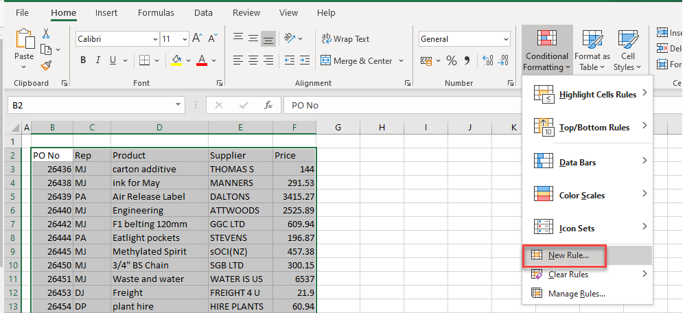
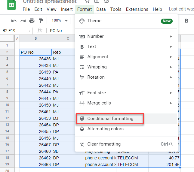
Firstly, choose the data on which you want to apply a conditional formatting tool other than the header. After choosing, press on the Home tab > Conditional Formatting > New Rule.

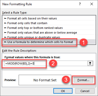
After that, you will see a dialog box named New Formatting Rule. Right from this dialog box, you have to choose the “Use a formula to determine which cells to format”. Choosing this option will let you add a formula to run the conditional formatting feature firmly. Now, you have to enter the formula in the box.
Here is the formula:
=MOD(ROW(B2),2)=0

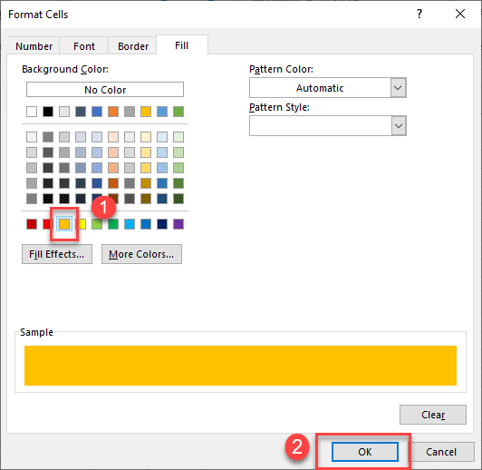
In the next step, where you need to color the alternate rows, you have to hit on the Format option. Fill and choose the color, now press OK.

Once again click on OK to get out of the rules box of conditional formatting. You will the application of your rule instantly.

Format Data as a Table
In Excel, most of the time people need to put data in a table format. Using tables in Excel comes up with loads of advantages. The most common one is that alternate colored rows are used to format data, which makes it attractive to others. When you need to change a range into a data table, firstly, you will have to choose the data and you have to choose the header as well.

Using Filter with Go To Special Feature
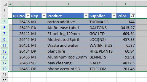
In the given example, you will see another column named Row Even/Odd. It is added to use Filter with Go To Special feature while understanding how to select every other row in Excel. For even row, you will see TRUE and for odd rows, you will see False.

Apart from that, you can even use the ISEVEN function. As given in the example, choose the F4 cell and apply your formula as mentioned below:
=ISEVEN(ROW())
Now, you will have to add the formula in the formula bar or else you can add it to the selected cell.

Press ENTER key and the fourth row has an even number that’s why you will see TRUE.

In the end, for all the other cells you may have to use the Fill Handle option to AutoFit formula.

Once it is done, follow these steps:
Choose the range where you need to add the Filter. In this example, all the columns are selected.
Later on, open the Data tab and choose Filter.

Furthermore, you can even try the CTRL + SHIFT + L keys right from your keyboard. These shortcut keys help you in applying the Filter to all the columns.

To activate the Filter option, choose the Row Odd/Even column, from which you can select the TRUE value to Filter. Now, click OK.

Keep in mind that when there are TRUE values, all the column values will be Filtered.

Now is the time to choose the range where you need to apply this GO To Special Feature.
For this, go to the Home tab, and choose Find & Select option from the Editing group. And select Go To Special feature.

You will see a dialog box, from which you need to choose the Visible cells only. Click OK and wind up the functioning.

VBA Automation
Whenever you don’t like to go for tricky ways, the ultimate solution to any problem is in VBA. Visual basic for applications is a built-in programming language in Excel. Similar to other functions, you can use it to select every other row in Excel automatically of a given range.
In the VBA Editor, you may have to copy and paste the script into the new module. For a new module, you need to go to Developer and then Visual Basic. If the Developer option is not activated, you will not see it on the ribbon. That’s why you have to activate it first to make it functional.
In the VBA Editor, click on the Insert and then Module
Sub SelectEveryOtherRow()
Dim userRange As Range
Dim alternateRowRange As Range
Dim rowCount, i As Long
Set userRange = Selection
rowCount = userRange.Rows.Count
With userRange
‘add row 1 of selected cells to the range variable
Set alternateRowRange = .Rows(1)
‘loop through every other row and add to range variable
For i = 3 To rowCount Step 2
Set alternateRowRange = Union(alternateRowRange, .Rows(i))
Next i
End With
‘select every other row
alternateRowRange.Select
End Sub
A selection of cells is needed to run this code. And the cells would be those you need to select every other row from first.
To Sum Up
In this post, you have found all the possible ways that can help in selection of every other row in Excel. Along with VBA coding, now the options are increased to select every other row in Excel. Try these different approaches to fulfill your needs.
In this post I will show you how to select every other row in Excel. Like many tasks in Excel, there is more than one way to achieve this. Here I show you 5 ways to select every other row in Excel. These 5 tips will improve your data manipulation skills.
Use the contents table below to skip to each section.
- Using CTRL and mouse click
- Conditional Formatting
- Format Data as a Table
- ‘Go To Special’ hack
- VBA (automation)
Using CTRL and Mouse Click To Select Every Other Row
The simplest way to select every other row in Excel is to hold down down the CTRL button on your keyboard (⌘ on MAC) and then the number of the rows you want to select.
Clicking on the row number itself highlights the whole row. By holding down CTRL, we are able to select every other row or even a bunch of single cells. This sort of selection is referred to as a non-contiguous range.

To deselect a row, simply click on it again. You can also perform a non-contiguous selection on individual cells and columns.
The advantage of this technique is it’s speed. You can very quickly select the rows you want to alter and then apply the change to all of them in one go.
The downside to this technique is when you have large datasets and it becomes too laborious to select all the rows you want manually.
You can also see from our example that the row selection exceeds the boundaries of our data which is also something you may not want to do.
Highlight Every Other Row With Conditional Formatting
Conditional formatting alters the look of a cell based upon the value within it. It is a very flexible tool and we can use it to highlight every other row in a data set. We can use it to highlight (select) every other row in Excel.
In this example, I want to color alternate rows, starting with the first row after the header.
First I select the data I want to apply the Conditional Formatting to (excluding the header), then hit:
Home –> Conditional Formatting –> New Rule…

Doing this will bring up the New Formatting Rule dialog box. From the options available, click on ‘Use a formula to determine which cells to format’.
This will change the dialog box to allow you to enter a formula that your conditional formatting will abide by. In the box, insert the following formula:
=MOD(ROW(B2),2)=0
NOTE: Substitute B2 above for the top-left most cell in your selection.

Formula Explainer
The MOD function returns the remainder of a division expression. So if you passed in the number 3 to be divided by 2, you’d get 1.
The ROW function returns the number of the row of the cell reference that you pass in. So in this case, cell B2 is row number 2.
So by passing in the row number, and dividing it by 2 using the MOD function, we’ll be able to tell if a row number is odd or even. Odd row numbers will return 1, even row numbers will return 0.
When the formula evaluates to 0, our conditional formatting rule is applied!
Next you can set the color of that you’d like the alternate rows to be. To do this, simply click ‘Format…’ –> Fill and select your chosen color. Then hit OK.

Click OK again to exit out of the Conditional Formatting rules dialog box and your rule will be applied immediately to your selection.

Format Data As A Table
Excel has a built-in feature to format ranges as tables. There are many advantages to using tables in Excel and you can learn more about using them from this great post by Easy Excel on Data Tables In Excel.
One of those benefits is that the data is formatted nicely with alternate colored rows, making it simpler for us to eye over the data.
To convert a range to a data table, first select the data, including a header if you have one, and then click:

Keyboard Shortcut
To quickly insert a table, select your data, then press CTRL + T on the keyboard.
The ‘Create Table’ dialog box will appear. Double-check that the range of cells you are going to format as a table is correct.
If you need to make an adjustment, you can overwrite the cell range in the box or simply click the small upward arrow, and then select the cells from your worksheet using the mouse.
If you data has headers, make sure the ‘My table has headers’ box is checked. Click OK.

Your data will now be formatted as a table object. The default color formatting will be applied and every other row will be colored.

You can quickly adjust the color formatting by selecting any cell within your data table and then clicking Table Design up on the ribbon.
In the ‘Table Styles’ section, you have the option to change the table’s color from a selection of pre-set formats. Customization is also available.

‘Go To Special’ Hack
This technique works great if you want to select every other row in Excel within your data set to then delete it.
First we create a “helper” column in the first column to the left of our data set. Give it a header to clearly mark it’s purpose, it will be deleted later on.
In the first row of the helper column, insert an ‘X’. Then click on this cell and drag your mouse down to the cell below, so that both of the cells are now selected.

Now the first to cells are selected, notice the small green square in the bottom-right of the selected cells – this is the Auto Fill Handle.
Click and hold the Auto Fill Handle, and drag the mouse down to extend the selection to all of the rows in your data set.

Auto Fill Handle
The cursor changes to a small black plus sign when you mouse over the auto fill handle to indicate it is active.
Clicking and dragging down will extend the “X then blank” pattern to all of the cells you select.
Alternatively, you can double-click the fill handle and it will automatically extend down to the end of your data set.
The auto fill handle is a really useful feature on Excel. You can read more about it’s functionality in this post on 6 Ways To Use The Fill Handle In Excel
Now we have created a recognizable pattern of “X then blank” for every 2 cells in the helper column. With these cells still selected, click:
Home –> Find & Select –> Go To Special…
This will open the ‘Go To Special’ dialog box. Select the ‘Blanks’ radio button then click OK.

Excel will now create a non-contiguous cell selection on the blank cells in the helper column. Now we can right-click on any of the selected cells and click Delete. This will launch the ‘Delete’ dialog box where you can then select Entire Row and then click OK.
Every other row will be deleted and the data will be pushed up into the gaps.


You can now delete your helper column
VBA (Automation)
VBA (visual basic for applications) is Excel’s built-in programming language. We can use this small script to automatically select every other row of a given range.
To use the script, copy and paste it into a new module in the VBA Editor.
To open a new module, go to Developer –> Visual Basic. If you don’t see the Developer tab on the ribbon, you’ll need to activate it first.
When in the VBA Editor, click Insert –> Module
Sub SelectEveryOtherRow()
Dim userRange As Range
Dim alternateRowRange As Range
Dim rowCount, i As Long
Set userRange = Selection
rowCount = userRange.Rows.Count
With userRange
Set alternateRowRange = .Rows(1)
For i = 3 To rowCount Step 2
Set alternateRowRange = Union(alternateRowRange, .Rows(i))
Next i
End With
alternateRowRange.Select
End Sub
To run this code, a user will need to make a selection of cells that they want to select every other row from first. The code works by looping through the selected range and adds every other row to a range variable which is then selected at the end of the programme.
Summary
Here we have looked at 5 different ways to select every other row in Excel. As we have seen, there are many methods available for us to do this from conditional formatting to automated selection via VBA.
These everyday tasks are unavoidable for those who use Excel to perform some routine activities in their workplace. However, those who fulfill these activities need to work smartly to perform those regular tasks. There is no better smart way to perform everyday tasks than shortcut keys. So, we all perform one activity, “selecting rows” in Excel. So, in this article, we will show you some of the circumstances where we can use the shortcut key to select the row in Excel.
Table of contents
- Select Row Shortcut in Excel
- General Scenarios of Selecting a Row in Excel
- How to Select a Row?
- Shortcut Way of Selecting Row in Excel
- Things to Remember Here
- Recommended Articles
General Scenarios of Selecting a Row in Excel
Selecting a row or column differs from case to case. So, let us illustrate some of the cases here.
- Deleting a Particular Row: If we want to get rid of a particular row or several rows, we usually need to select those rows and delete the selected rows.
- Inserting a New Row: Like how we need to select rows before deleting them similarly, we need to choose columns or columns to insert the new one. Suppose we choose and press the “Insert” option. It will insert only one column. These new rows will be inserted with as many numbers of columns as selected.
- Formatting a Row: If we want to apply any specific formatting to a particular row(s), we need to select the row and use the formatting as per our liking.
You are free to use this image on your website, templates, etc, Please provide us with an attribution linkArticle Link to be Hyperlinked
For eg:
Source: Excel Shortcut to Select Row (wallstreetmojo.com)
How to Select a Row?
Below is an example of using the keyboard shortcut keyAn Excel shortcut is a technique of performing a manual task in a quicker way.read more to select a row in excel.
You can download this Shortcut to Select Row Excel Template here – Shortcut to Select Row Excel Template
For beginners, selecting a row is often performed manually. But to work productively, we need to use shortcut keys. Before that, let us recollect the manual ways of selecting a row.
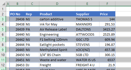
- For example, let us look at the below data set.
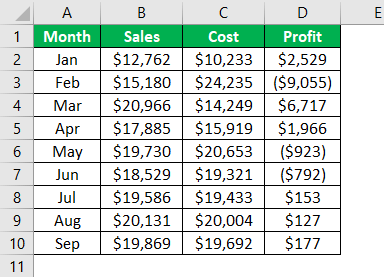
- If we want to select row number 4, we need to place a cursor on the row header (numerical header), then we should see a small arrow key.
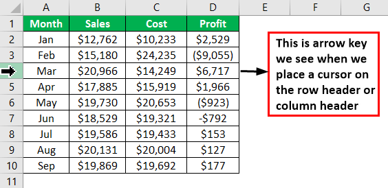
- As soon as we see the arrow key, we must press the left key of the mouse, and it will select the targeted row.
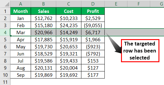
After selecting the row, we can press different shortcut keys depending on requirements like “inserting a new row,” “deleting the row,” and “choosing other rows below or above.”
Shortcut Way of Selecting Row in Excel
We want to mention that there is no major difference between selecting the row manually and selecting the row using the shortcut. The only difficulty here is that we need to move our hands from the keyboard to the mouse. But once we get the hang of shortcut keys, we may start loving them.
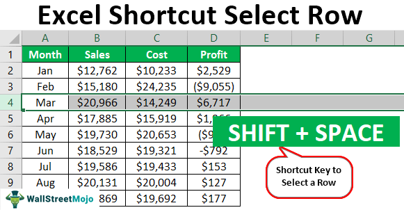
The Shortcut Key to Select a Row:
![]()
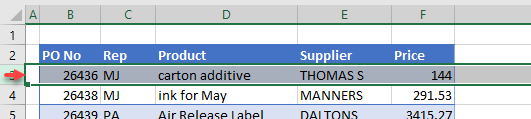
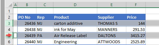
- For example, take the above data table only to illustrate this example. Assume we want to select row number 4, so we must choose any of the cells from this row first.
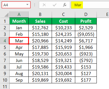
- We have chosen the A4 cell in row number 4. Now, press the “Spacebar” by holding the “Shift” key.
So as soon as we have pressed the shortcut key, it has selected the entire row of the active cell (the active cell was the A4 cell).
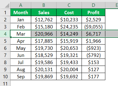
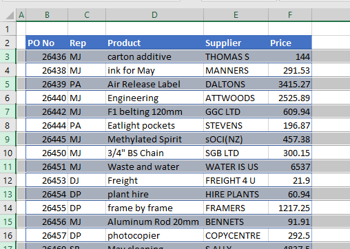
- Now assume after selecting row number 4, we need to select all the rows below the selected row, then we can press another shortcut key, “Shift + Ctrl + Down Arrow.”
![]()
- So the moment we press this, it may select all the rows below the selected row.
Suppose we press “Shift + Ctrl + Down Arrow” one more time; it may take us to the next non-break cell or row.
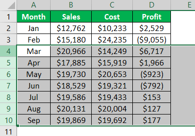
Similarly, if we want to select all the rows above the selected row, we must press the shortcut key “Shift + Ctrl + Up Arrow.“
Things to Remember Here
- We must select the cell in that particular row to select the row before pressing the shortcut key.
- We need to press the shortcut key in order, i.e., “Shift” and then “Space.”
Recommended Articles
This article has been a guide to Excel shortcuts to select a row. We discuss using the keyboard shortcut key to select a row in Excel, examples, and a downloadable Excel template. You may learn more about Excel from the following articles: –
- Edit Cell Using Excel Shortcut
- Excel Degrees Function
- Count Number of Excel Rows & Columns
- Group Rows in Excel
- Split Panes in Excel
See all How-To Articles
This tutorial demonstrates how to select every other row in Excel and Google Sheets.
When you’re working with data in Excel, you have a need to select the data in every other row. There are a few ways to select every other row.
Select Every Other Row
Keyboard and Mouse
- Click on the row header to select the first row.
- Holding down the CTRL key on the keyboard, click in the row header of the second row.
- With the CTRL key still held down, click on every other row header until all the rows you need are selected.
Cell Format and Filter
You can use Format as Table and filtering to select every other row.
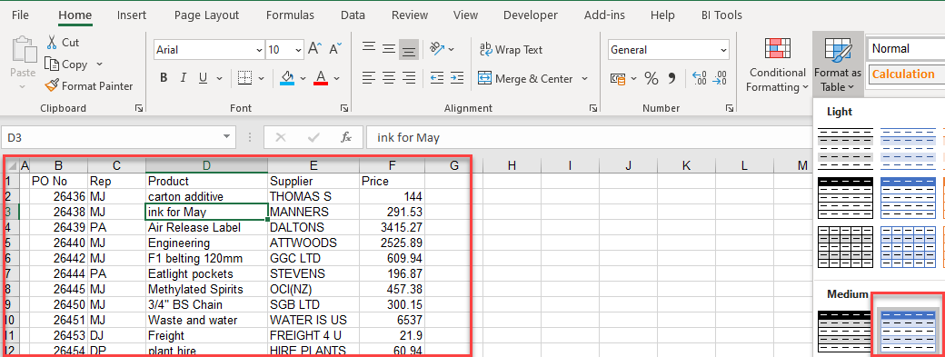
- Highlight the cells whose rows you wish to select. In the Ribbon, go to Home > Cells > Format as Table and select the formatting.
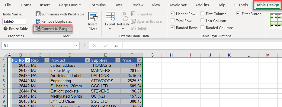
- Then, to remove the table, in the Ribbon, select Table > Convert to Range.
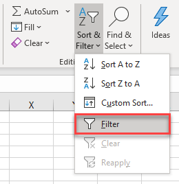
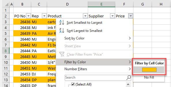
- Next, in the Ribbon, select Home > Editing > Sort & Filter > Filter.
- Click the drop-down arrow on any of the column headings and select Filter by Color.
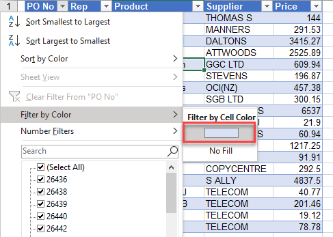
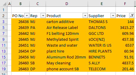
- Every second row is now filtered for. Select these rows.
Conditional Formatting and Filter
You can use Conditional Formatting and Filtering to select every other row.
- Highlight the cells whose rows you wish to select. In the Ribbon, go to Home > Cells >Conditional Formatting.
- Select (1) Use a formula to determine which cells to format and then (2) enter the formula:
=MOD(ROW(B3),2)=0Then (3) click on Format…
- The ROW Function returns the row number of the cell.
- The MOD Function, here, tests whether a number is even or odd by returning the remainder of the ROW formula divided by 2.
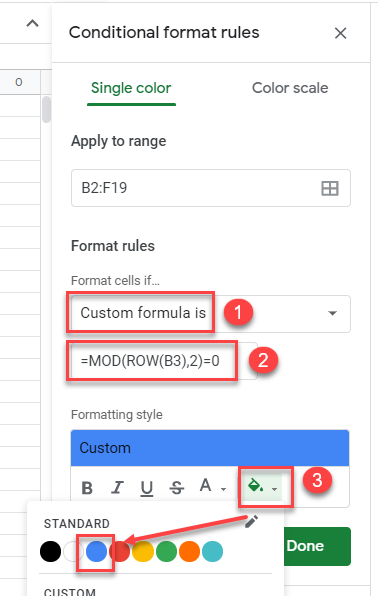
- In the Fill tab, select the color to format each alternate row, and click OK.
- Click OK again to apply the formatting to your worksheet.
- As with Format as a Table, you can now Filter by Color to select every alternate row.
All the rows with the yellow cells are shown.
Select Every Other Row in Google Sheets
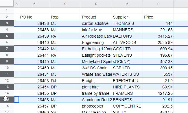
As with Excel, you can select every other row in a Google Sheet by selecting the first row and then holding down the CTRL key and selecting each alternate row thereafter.
You can also use conditional formatting and filtering to select every other row.
- Highlight the cells whose rows you wish to select. In the Menu, select Format > Conditional Formatting.
- Select (1) Custom formula is from the Format cells if… list and then (2) type in the following formula:
=MOD(ROW(B3),2)=0Then (3) select the color you wish every other row in the selection to be formatted with.
- Click Done to format the sheet.
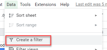
- Then create a filter to filter the rows by color.
In the Menu, select Data > Create a filter.
- In the filter drop-down list at the top of one of the columns, select Filter by Color > Fill Color and then select which color to filter on.
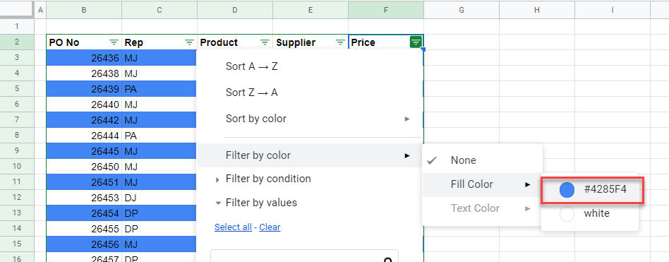
Every other row is now shown.
See also: How to Display Data With Banded Rows
In this article, we will learn How to use the keyboard multiple select entire row in Excel.
Scenario:
In Excel, selecting cells is a common practice in Excel. It helps you perform many tasks like addition, deletion and width adjustment on selected multiple rows and columns. While applying the formula on data in Excel, either we can manually input or use cell reference and keyboard shortcut. Keyboard Shortcut keys to select all rows and columns can provide an easier and quicker method for using Excel.
Shortcut method to select entire row/column in Excel
First select the cell / cells where you want to select the entire row or column and then choose either of the options mentioned below.
- Use Ctrl + Space shortcut keys from your keyboard to select the columns
- Use Shift + Space shortcut keys from your keyboard to select the rows
Example :
All of these might be confusing to understand. Let’s understand how to use the function using an example. Here we have sample data and below is the method which will show you how to select the entire column or row using the excel keyboard.
Now Selecting Rows:
Select the cell, you wish to select.
Press Shift+ Space key to select the row on the selected cell (release the keys, if the row is selected).

If you wish to select the adjacent rows with the selected row, press Shift+ Up/down arrow key(s) to select the UP or DOWN to that row. You can go either way but can’t access both sides of it.
Selecting 3rd to 5th whole rows of the sheet can be done in two ways:
Select any cell of the 3rd row, press Shift + Space key to select the row.
Now use the Shift + Down(twice) arrow key to select the 4th and the 5th row.
Or you could go another way from 5th to 3rd row but you won’t be able to select 3rd and 5th row both, starting from the 4th row.
Select multiple rows and columns of a table with shortcut keys and perform your tasks efficiently.
Now selecting Column:
Select the cell, you wish to select.
Use Ctrl + Space shortcut keys from your keyboard to select the column as shown below in the picture.

If you wish to select the adjacent columns with the selected column, use Shift + Left/Right arrow key(s) to select the left or right side of that column. You can go either way but can’t access both sides of it.
We need to select 3rd to 5th columns.
Select any cell of the 3rd column.
Use Ctrl + Space shortcut keys from your keyboard to select the column (Leave the keys if the column is selected).
Now use Shift + Right (twice) arrow keys to select the 4th and the 5th column simultaneously.
You could go another way from 5th to 3rd column but you won’t be able to select 3rd and 5th column both, starting from the 4th column as it allows you to move or edit in one direction.

As you can see all the selected columns in the image above.
Asked Question:
How to apply formula to the entire column?
Easy, write formula in the first cell of the column and press CTRL + SPACE to select the entire column and then CTRL+D to apply formula to the entire column.
How to select all in excel?
To select all data press CTRL+A.
How to select multiple cells in excel mac?
Hold down the command key and scroll over the cells to select. If the cells are not adjacent then click on the cell while holding the command key.
Here are all the observational notes using the formula in Excel
Notes :
- You can select a single cell or range of consecutive cells. But cannot apply the shortcut to select different columns or rows located separately.
- You can go either way from the first selected row/column using Shift + arrow keys.
Hope this article about How to use keyboard multiple select entire row w/o click and drag in Excel is explanatory. Find more articles on calculating values and related Excel formulas here. If you liked our blogs, share it with your friends on Facebook. And also you can follow us on Twitter and Facebook. We would love to hear from you, do let us know how we can improve, complement or innovate our work and make it better for you. Write to us at info@exceltip.com.
Related Articles :
Paste Special Shortcut in Mac and Windows : In windows, the keyboard shortcut for paste special is Ctrl + Alt + V. Whereas in Mac, use Ctrl + COMMAND + V key combination to open the paste special dialog in Excel.
How to Insert Row Shortcut in Excel : Use Ctrl + Shift + = to open the Insert dialog box where you can insert row, column or cells in Excel.
How to Select Entire Column and Row Using Keyboard Shortcuts in Excel : Selecting cells is a very common function in Excel.Use Ctrl + Space to select whole column and Shift + Space to select whole row using keyboard shortcut in Excel
Excel Shortcut Keys for Merge and Center : This Merge and Center shortcut helps you quickly merge and unmerge cells.
How to use the Shortcut To Toggle Between Absolute and Relative References in Excel : F4 shortcut to convert absolute to relative reference and same shortcut use for vice versa in Excel.
How to use Shortcut Keys for Merge and Center in Excel : Use Alt and then follow h, m and c to Merge and centre cells in Excel.
How to use Shortcut Keys for Sort & filter in Excel : Use Ctrl + Shift + L from keyboard to apply sort and filter on table in Excel.
Popular Articles :
50 Excel Shortcuts to Increase Your Productivity : Get faster at your tasks in Excel. These shortcuts will help you increase your work efficiency in Excel.
How to use the VLOOKUP Function in Excel : This is one of the most used and popular functions of excel that is used to lookup value from different ranges and sheets.
How to use the IF Function in Excel : The IF statement in Excel checks the condition and returns a specific value if the condition is TRUE or returns another specific value if FALSE.
How to use the SUMIF Function in Excel : This is another dashboard essential function. This helps you sum up values on specific conditions.
How to use the COUNTIF Function in Excel : Count values with conditions using this amazing function. You don’t need to filter your data to count specific values. Countif function is essential to prepare your dashboard.
VBA Select
It is very common to find the .Select methods in saved macro recorder code, next to a Range object.
.Select is used to select one or more elements of Excel (as can be done by using the mouse) allowing further manipulation of them.
Selecting cells with the mouse:
Selecting cells with VBA:
    'Range([cell1],[cell2])
    Range(Cells(1, 1), Cells(9, 5)).Select
    Range("A1", "E9").Select
    Range("A1:E9").Select
Each of the above lines select the range from «A1» to «E9».
VBA Select CurrentRegion
If a region is populated by data with no empty cells, an option for an automatic selection is the CurrentRegion property alongside the .Select method.
CurrentRegion.Select will select, starting from a Range, all the area populated with data.
Range("A1").CurrentRegion.Select
Make sure there are no gaps between values, as CurrentRegion will map the region through adjoining cells (horizontal, vertical and diagonal).
Range("A1").CurrentRegion.SelectWith all the adjacent data
Not all adjacent data
«C4» is not selected because it is not immediately adjacent to any filled cells.
VBA ActiveCell
The ActiveCell property brings up the active cell of the worksheet.
In the case of a selection, it is the only cell that stays white.
A worksheet has only one active cell.
    Range("B2:C4").Select
    ActiveCell.Value = "Active"
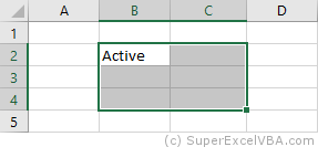
Usually the ActiveCell property is assigned to the first cell (top left) of a Range, although it can be different when the selection is made manually by the user (without macros).
The AtiveCell property can be used with other commands, such as Resize.
VBA Selection
After selecting the desired cells, we can use Selection to refer to it and thus make changes:
    Range("A1:D7").Select
    Selection = 7
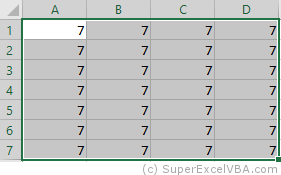
Selection also accepts methods and properties (which vary according to what was selected).
    Selection.ClearContents 'Deletes only the contents of the selection
    Selection.Interior.Color = RGB(255, 255, 0) 'Adds background color to the selection
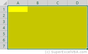
As in this case a cell range has been selected, the Selection will behave similarly to a Range. Therefore, Selection should also accept the .Interior.Color property.
RGB (Red Green Blue) is a color system used in a number of applications and languages. The input values for each color, in the example case, ranges from 0 to 255.
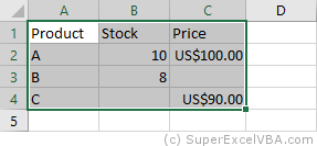
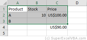
Selection FillDown
If there is a need to replicate a formula to an entire selection, you can use the .FillDown method
Selection.FillDown
Before the FillDown
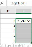
After the FillDown
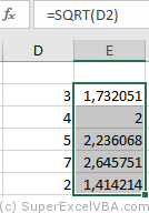
.FillDown is a method applicable to Range. Since the Selection was done in a range of cells (equivalent to a Range), the method will be accepted.
.FillDown replicates the Range/Selection formula of the first line, regardless of which ActiveCell is selected.
.FillDown can be used at intervals greater than one column (E.g. Range(«B1:C2»).FillDown will replicate the formulas of B1 and C1 to B2 and C2 respectively).
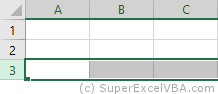
VBA EntireRow and EntireColumn
You can select one or multiple rows or columns with VBA.
    Range("B2").EntireRow.Select
    Range("C3:D3").EntireColumn.Select
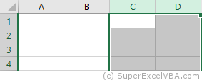
The selection will always refer to the last command executed with Select.
To insert a row use the Insert method.
    Range("A7").EntireRow.Insert
    'In this case, the content of the seventh row will be shifted downward
To delete a row use the Delete method.
    Range("A7").EntireRow.Delete
    'In this case, the content of the eighth row will be moved to the seventh
VBA Rows and Columns
Just like with the EntireRow and EntireColumn property, you can use Rows and Columns to select a row or column.
    Columns(5).Select
    Rows(3).Select
To hide rows:
Range("A1:C3").Rows.Hidden = True
In the above example, rows 1 to 3 of the worksheet were hidden.
VBA Row and Column
Row and Column are properties that are often used to obtain the numerical address of the first row or first column of a selection or a specific cell.
    Range("A3:H30").Row 'Referring to the row; returns 3
    Range("B3").Column  'Referring to the column; returns 2
The results of Row and Column are often used in loops or resizing.
Consolidating Your Learning
Suggested Exercise
SuperExcelVBA.com is learning website. Examples might be simplified to improve reading and basic understanding. Tutorials, references, and examples are constantly reviewed to avoid errors, but we cannot warrant full correctness of all content. All Rights Reserved.
Excel ® is a registered trademark of the Microsoft Corporation.
© 2023 SuperExcelVBA | ABOUT
![]()