Select from worksheet in excel - Word и Excel - помощь в работе с программами

Содержание

How to select cells/ranges by using Visual Basic procedures in Excel
How to Select a Cell on the Active Worksheet
How to Select a Cell on Another Worksheet in the Same Workbook
How to Select a Cell on a Worksheet in a Different Workbook
How to Select a Range of Cells on the Active Worksheet
How to Select a Range of Cells on Another Worksheet in the Same Workbook
How to Select a Range of Cells on a Worksheet in a Different Workbook
How to Select a Named Range on the Active Worksheet
How to Select a Named Range on Another Worksheet in the Same Workbook
How to Select a Named Range on a Worksheet in a Different Workbook
How to Select a Cell Relative to the Active Cell
How to Select a Cell Relative to Another (Not the Active) Cell
How to Select a Range of Cells Offset from a Specified Range
How to Select a Specified Range and Resize the Selection
How to Select a Specified Range, Offset It, and Then Resize It
How to Select the Union of Two or More Specified Ranges
How to Select the Intersection of Two or More Specified Ranges
How to Select the Last Cell of a Column of Contiguous Data
How to Select the Blank Cell at Bottom of a Column of Contiguous Data
How to Select an Entire Range of Contiguous Cells in a Column
How to Select an Entire Range of Non-Contiguous Cells in a Column
How to Select a Rectangular Range of Cells
How to Select Multiple Non-Contiguous Columns of Varying Length
Notes on the examples
Select cell contents in Excel
Select one or more cells
Select one or more rows and columns
Select table, list or worksheet
Need more help?
Select worksheets
Need more help?

How to select cells/ranges by using Visual Basic procedures in Excel

Microsoft provides programming examples for illustration only, without warranty either expressed or implied. This includes, but is not limited to, the implied warranties of merchantability or fitness for a particular purpose. This article assumes that you are familiar with the programming language that is being demonstrated and with the tools that are used to create and to debug procedures. Microsoft support engineers can help explain the functionality of a particular procedure, but they will not modify these examples to provide added functionality or construct procedures to meet your specific requirements. The examples in this article use the Visual Basic methods listed in the following table.

The examples in this article use the properties in the following table.

How to Select a Cell on the Active Worksheet

To select cell D5 on the active worksheet, you can use either of the following examples:

How to Select a Cell on Another Worksheet in the Same Workbook

To select cell E6 on another worksheet in the same workbook, you can use either of the following examples:

Or, you can activate the worksheet, and then use method 1 above to select the cell:

How to Select a Cell on a Worksheet in a Different Workbook

To select cell F7 on a worksheet in a different workbook, you can use either of the following examples:

Or, you can activate the worksheet, and then use method 1 above to select the cell:

How to Select a Range of Cells on the Active Worksheet

To select the range C2:D10 on the active worksheet, you can use any of the following examples:

How to Select a Range of Cells on Another Worksheet in the Same Workbook

To select the range D3:E11 on another worksheet in the same workbook, you can use either of the following examples:

Or, you can activate the worksheet, and then use method 4 above to select the range:

How to Select a Range of Cells on a Worksheet in a Different Workbook

To select the range E4:F12 on a worksheet in a different workbook, you can use either of the following examples:

Or, you can activate the worksheet, and then use method 4 above to select the range:

How to Select a Named Range on the Active Worksheet

To select the named range «Test» on the active worksheet, you can use either of the following examples:

How to Select a Named Range on Another Worksheet in the Same Workbook

To select the named range «Test» on another worksheet in the same workbook, you can use the following example:

Or, you can activate the worksheet, and then use method 7 above to select the named range:

How to Select a Named Range on a Worksheet in a Different Workbook

To select the named range «Test» on a worksheet in a different workbook, you can use the following example:

Or, you can activate the worksheet, and then use method 7 above to select the named range:

How to Select a Cell Relative to the Active Cell

To select a cell that is five rows below and four columns to the left of the active cell, you can use the following example:

To select a cell that is two rows above and three columns to the right of the active cell, you can use the following example:

An error will occur if you try to select a cell that is «off the worksheet.» The first example shown above will return an error if the active cell is in columns A through D, since moving four columns to the left would take the active cell to an invalid cell address.

How to Select a Cell Relative to Another (Not the Active) Cell

To select a cell that is five rows below and four columns to the right of cell C7, you can use either of the following examples:

How to Select a Range of Cells Offset from a Specified Range

To select a range of cells that is the same size as the named range «Test» but that is shifted four rows down and three columns to the right, you can use the following example:

If the named range is on another (not the active) worksheet, activate that worksheet first, and then select the range using the following example:

How to Select a Specified Range and Resize the Selection

To select the named range «Database» and then extend the selection by five rows, you can use the following example:

How to Select a Specified Range, Offset It, and Then Resize It

To select a range four rows below and three columns to the right of the named range «Database» and include two rows and one column more than the named range, you can use the following example:

How to Select the Union of Two or More Specified Ranges

To select the union (that is, the combined area) of the two named ranges «Test» and «Sample,» you can use the following example:

that both ranges must be on the same worksheet for this example to work. Note also that the Union method does not work across sheets. For example, this line works fine.

returns the error message:

Union method of application class failed

How to Select the Intersection of Two or More Specified Ranges

To select the intersection of the two named ranges «Test» and «Sample,» you can use the following example:

Note that both ranges must be on the same worksheet for this example to work.

Examples 17-21 in this article refer to the following sample set of data. Each example states the range of cells in the sample data that would be selected.

How to Select the Last Cell of a Column of Contiguous Data

To select the last cell in a contiguous column, use the following example:

When this code is used with the sample table, cell A4 will be selected.

How to Select the Blank Cell at Bottom of a Column of Contiguous Data

To select the cell below a range of contiguous cells, use the following example:

When this code is used with the sample table, cell A5 will be selected.

How to Select an Entire Range of Contiguous Cells in a Column

To select a range of contiguous cells in a column, use one of the following examples:

When this code is used with the sample table, cells A1 through A4 will be selected.

How to Select an Entire Range of Non-Contiguous Cells in a Column

To select a range of cells that are non-contiguous, use one of the following examples:

When this code is used with the sample table, it will select cells A1 through A6.

How to Select a Rectangular Range of Cells

In order to select a rectangular range of cells around a cell, use the CurrentRegion method. The range selected by the CurrentRegion method is an area bounded by any combination of blank rows and blank columns. The following is an example of how to use the CurrentRegion method:

This code will select cells A1 through C4. Other examples to select the same range of cells are listed below:

In some instances, you may want to select cells A1 through C6. In this example, the CurrentRegion method will not work because of the blank line on Row 5. The following examples will select all of the cells:

How to Select Multiple Non-Contiguous Columns of Varying Length

To select multiple non-contiguous columns of varying length, use the following sample table and macro example:

When this code is used with the sample table, cells A1:A3 and C1:C6 will be selected.

Notes on the examples

The ActiveSheet property can usually be omitted, because it is implied if a specific sheet is not named. For example, instead of

The ActiveWorkbook property can also usually be omitted. Unless a specific workbook is named, the active workbook is implied.

When you use the Application.Goto method, if you want to use two Cells methods within the Range method when the specified range is on another (not the active) worksheet, you must include the Sheets object each time. For example:

For any item in quotation marks (for example, the named range «Test»), you can also use a variable whose value is a text string. For example, instead of

Источник

Select cell contents in Excel

In Excel, you can select cell contents of one or more cells, rows and columns.

Note: If a worksheet has been protected, you might not be able to select cells or their contents on a worksheet.

Select one or more cells

Click on a cell to select it. Or use the keyboard to navigate to it and select it.

To select a range, select a cell, then with the left mouse button pressed, drag over the other cells.

Or use the Shift + arrow keys to select the range.

To select non-adjacent cells and cell ranges, hold Ctrl and select the cells.

Select one or more rows and columns

Select the letter at the top to select the entire column. Or click on any cell in the column and then press Ctrl + Space.

Select the row number to select the entire row. Or click on any cell in the row and then press Shift + Space.

To select non-adjacent rows or columns, hold Ctrl and select the row or column numbers.

Select table, list or worksheet

To select a list or table, select a cell in the list or table and press Ctrl + A.

To select the entire worksheet, click the Select All button at the top left corner.

Note: In some cases, selecting a cell may result in the selection of multiple adjacent cells as well. For tips on how to resolve this issue, see this post How do I stop Excel from highlighting two cells at once? in the community.

Click the cell, or press the arrow keys to move to the cell.

A range of cells

Click the first cell in the range, and then drag to the last cell, or hold down SHIFT while you press the arrow keys to extend the selection.

You can also select the first cell in the range, and then press F8 to extend the selection by using the arrow keys. To stop extending the selection, press F8 again.

A large range of cells

Click the first cell in the range, and then hold down SHIFT while you click the last cell in the range. You can scroll to make the last cell visible.

All cells on a worksheet

Click the Select All button.

To select the entire worksheet, you can also press CTRL+A.

Note: If the worksheet contains data, CTRL+A selects the current region. Pressing CTRL+A a second time selects the entire worksheet.

Nonadjacent cells or cell ranges

Select the first cell or range of cells, and then hold down CTRL while you select the other cells or ranges.

You can also select the first cell or range of cells, and then press SHIFT+F8 to add another nonadjacent cell or range to the selection. To stop adding cells or ranges to the selection, press SHIFT+F8 again.

Note: You cannot cancel the selection of a cell or range of cells in a nonadjacent selection without canceling the entire selection.

An entire row or column

Click the row or column heading.

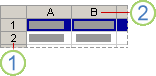
2. Column heading

You can also select cells in a row or column by selecting the first cell and then pressing CTRL+SHIFT+ARROW key (RIGHT ARROW or LEFT ARROW for rows, UP ARROW or DOWN ARROW for columns).

Note: If the row or column contains data, CTRL+SHIFT+ARROW key selects the row or column to the last used cell. Pressing CTRL+SHIFT+ARROW key a second time selects the entire row or column.

Adjacent rows or columns

Drag across the row or column headings. Or select the first row or column; then hold down SHIFT while you select the last row or column.

Nonadjacent rows or columns

Click the column or row heading of the first row or column in your selection; then hold down CTRL while you click the column or row headings of other rows or columns that you want to add to the selection.

The first or last cell in a row or column

Select a cell in the row or column, and then press CTRL+ARROW key (RIGHT ARROW or LEFT ARROW for rows, UP ARROW or DOWN ARROW for columns).

The first or last cell on a worksheet or in a Microsoft Office Excel table

Press CTRL+HOME to select the first cell on the worksheet or in an Excel list.

Press CTRL+END to select the last cell on the worksheet or in an Excel list that contains data or formatting.

Cells to the last used cell on the worksheet (lower-right corner)

Select the first cell, and then press CTRL+SHIFT+END to extend the selection of cells to the last used cell on the worksheet (lower-right corner).

Cells to the beginning of the worksheet

Select the first cell, and then press CTRL+SHIFT+HOME to extend the selection of cells to the beginning of the worksheet.

More or fewer cells than the active selection

Hold down SHIFT while you click the last cell that you want to include in the new selection. The rectangular range between the active cell and the cell that you click becomes the new selection.

Need more help?

You can always ask an expert in the Excel Tech Community or get support in the Answers community.

Источник

Select worksheets

By clicking the sheet tabs at the bottom of the Excel window, you can quickly select one or more sheets. To enter or edit data on several worksheets at the same time, you can group worksheets by selecting multiple sheets. You can also format or print a selection of sheets at the same time.

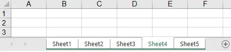
Click the tab for the sheet you want to edit. The active sheet will be a different color than other sheets. In this case, Sheet4 has been selected.

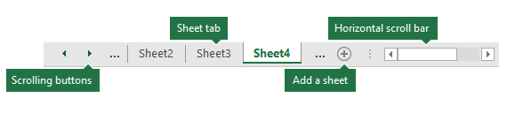
If you don’t see the tab that you want, click the scrolling buttons to locate the tab. You can add a sheet by pressing the Add Sheet button to the right of the sheet tabs.

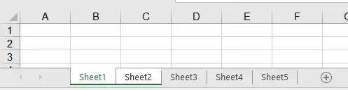
Two or more adjacent sheets

Click the tab for the first sheet, then hold down SHIFT while you click the tab for the last sheet that you want to select.

By keyboard: First, press F6 to activate the sheet tabs. Next, use the left or right arrow keys to select the sheet you want, then you can use Ctrl+Space to select that sheet. Repeat the arrow and Ctrl+Space steps to select additional sheets.

Two or more nonadjacent sheets

Click the tab for the first sheet, then hold down CTRL while you click the tabs of the other sheets that you want to select.

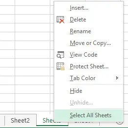
All sheets in a workbook

Right-click a sheet tab, and then click the Select All Sheets option.

TIP: After choosing multiple sheets, [Group] appears in the title bar at the top of the worksheet. To cancel a selection of multiple worksheets in a workbook, click any unselected worksheet. If no unselected sheet is visible, right-click the tab of a selected sheet, and then click Ungroup Sheets on the shortcut menu.

Data that you enter or edit in the active worksheet will appear in all selected sheets. These changes might replace data on the active sheet and—perhaps unintentionally—on other selected sheets.

Data that you copy or cut in grouped sheets cannot be pasted onto another sheet, because the size of the copy area includes all layers of the selected sheets (which is different from the paste area in a single sheet). It’s important to ensure that only one sheet is selected before you copy or move data to another worksheet.

When you save a workbook that contains grouped sheets and then close the workbook, the sheets that you selected remain grouped when you reopen that workbook.

In Excel for the web you can’t select more than one sheet at a time, but it’s easy to find the sheet you want.

Select the All Sheets menu, then choose a sheet from the menu to open it.

From the sheets listed along the bottom, select a sheet name to open it. Use the arrows just beside the All Sheets menu to scroll forward and backward through sheets to review ones that aren’t currently visible.

Need more help?

You can always ask an expert in the Excel Tech Community or get support in the Answers community.

Источник

Select cell contents in Excel

In Excel, you can select cell contents of one or more cells, rows and columns.

Note: If a worksheet has been protected, you might not be able to select cells or their contents on a worksheet.

Select one or more cells

Click on a cell to select it. Or use the keyboard to navigate to it and select it.
To select a range, select a cell, then with the left mouse button pressed, drag over the other cells.

Or use the Shift + arrow keys to select the range.
To select non-adjacent cells and cell ranges, hold Ctrl and select the cells.

Select one or more rows and columns

Select the letter at the top to select the entire column. Or click on any cell in the column and then press Ctrl + Space.
Select the row number to select the entire row. Or click on any cell in the row and then press Shift + Space.
To select non-adjacent rows or columns, hold Ctrl and select the row or column numbers.

Select table, list or worksheet

To select a list or table, select a cell in the list or table and press Ctrl + A.
To select the entire worksheet, click the Select All button at the top left corner.

Note: In some cases, selecting a cell may result in the selection of multiple adjacent cells as well. For tips on how to resolve this issue, see this post How do I stop Excel from highlighting two cells at once? in the community.

To select	Do this
A single cell	Click the cell, or press the arrow keys to move to the cell.
A range of cells	Click the first cell in the range, and then drag to the last cell, or hold down SHIFT while you press the arrow keys to extend the selection. You can also select the first cell in the range, and then press F8 to extend the selection by using the arrow keys. To stop extending the selection, press F8 again.
A large range of cells	Click the first cell in the range, and then hold down SHIFT while you click the last cell in the range. You can scroll to make the last cell visible.
All cells on a worksheet	Click the Select All button. To select the entire worksheet, you can also press CTRL+A. Note: If the worksheet contains data, CTRL+A selects the current region. Pressing CTRL+A a second time selects the entire worksheet.
Nonadjacent cells or cell ranges	Select the first cell or range of cells, and then hold down CTRL while you select the other cells or ranges. You can also select the first cell or range of cells, and then press SHIFT+F8 to add another nonadjacent cell or range to the selection. To stop adding cells or ranges to the selection, press SHIFT+F8 again. Note: You cannot cancel the selection of a cell or range of cells in a nonadjacent selection without canceling the entire selection.
An entire row or column	Click the row or column heading. 1. Row heading 2. Column heading You can also select cells in a row or column by selecting the first cell and then pressing CTRL+SHIFT+ARROW key (RIGHT ARROW or LEFT ARROW for rows, UP ARROW or DOWN ARROW for columns). Note: If the row or column contains data, CTRL+SHIFT+ARROW key selects the row or column to the last used cell. Pressing CTRL+SHIFT+ARROW key a second time selects the entire row or column.
Adjacent rows or columns	Drag across the row or column headings. Or select the first row or column; then hold down SHIFT while you select the last row or column.
Nonadjacent rows or columns	Click the column or row heading of the first row or column in your selection; then hold down CTRL while you click the column or row headings of other rows or columns that you want to add to the selection.
The first or last cell in a row or column	Select a cell in the row or column, and then press CTRL+ARROW key (RIGHT ARROW or LEFT ARROW for rows, UP ARROW or DOWN ARROW for columns).
The first or last cell on a worksheet or in a Microsoft Office Excel table	Press CTRL+HOME to select the first cell on the worksheet or in an Excel list. Press CTRL+END to select the last cell on the worksheet or in an Excel list that contains data or formatting.
Cells to the last used cell on the worksheet (lower-right corner)	Select the first cell, and then press CTRL+SHIFT+END to extend the selection of cells to the last used cell on the worksheet (lower-right corner).
Cells to the beginning of the worksheet	Select the first cell, and then press CTRL+SHIFT+HOME to extend the selection of cells to the beginning of the worksheet.
More or fewer cells than the active selection	Hold down SHIFT while you click the last cell that you want to include in the new selection. The rectangular range between the active cell and the cell that you click becomes the new selection.

Need more help?

You can always ask an expert in the Excel Tech Community or get support in the Answers community.

VBA Select Worksheet Method — Sheet Object in Excel

VBA Select Worksheet method is used to select a cell or a range(collection of cells). Here we are using Select method of worksheet object to select any cell or a range. It is very frequently used method while writing VBA macros, but before selecting any cell or range first activate cell or that particular range which u want to select. Otherwise sometimes it will fail unless your procedure activates the worksheet before using the Select method of worksheet object.

When we use Select Worksheet Method in VBA?
VBA Select Worksheet Method: Syntax
VBA Select Worksheet Method: Example 1
VBA Select Worksheet Method: Example 2
VBA Select Worksheet Method: Instructions

When we use Select Worksheet Method in VBA?

If we want to selects any single cell or collection of cells, then we use select worksheet method. You can use activate method of worksheet object to make a single cell as active cell.

VBA Select Worksheet Method: Syntax

Here is the example syntax to Select Worksheet using VBA. You can use either a Worksheet name or Worksheet number. Always best practice is to use sheet name.

Worksheets(“Your Worksheet Name”). Select(

[Replace])
‘Or
Sheets(“Worksheet Number”).Select([Replace])

Where Replace is the Optional parameter. When the value is True, it will replace the current selection. When the value is False, it will extend the current selection.
Select is the method of Workbook object is used to makes current sheet as active sheet.

VBA Select Worksheet Method: Example 1

Please see the below VBA procedure. In this procedure we are activating and selecting a Range(“A1”) in the worksheet named “Project1”.

Sub Select_Range()
    Worksheets("Project1").Activate
    Range("A1").Select
End Sub

VBA Select Worksheet Method: Example 2

Please see the below VBA code or macro procedure to Select Worksheet. In this example we are activating first Worksheet in the active workbook.

Sub Select_Range()
    Worksheets(1).Activate
    Range("A1").Select
End Sub

VBA Select Worksheet Method: Instructions

Please follow the below step by step instructions to execute the above mentioned VBA macros or codes:

Open an Excel Worksheet
Press Alt+F11 to Open VBA Editor
Insert a Module from Insert Menu
Copy the above code for activating worksheet and Paste in the code window(VBA Editor)
Save the file as macro enabled Worksheet
Press ‘F5’ to run it or Keep Pressing ‘F8’ to debug the code line by line and observe the selection.

Effortlessly Manage Your Projects and Resources

120+ Professional Project Management Templates!

A Powerful & Multi-purpose Templates for project management. Now seamlessly manage your projects, tasks, meetings, presentations, teams, customers, stakeholders and time. This page describes all the amazing new features and options that come with our premium templates.

Save Up to 85% LIMITED TIME OFFER

All-in-One Pack
120+ Project Management Templates

Essential Pack
50+ Project Management Templates

Excel Pack
50+ Excel PM Templates

PowerPoint Pack
50+ Excel PM Templates

MS Word Pack
25+ Word PM Templates

Ultimate Project Management Template

Ultimate Resource Management Template

Project Portfolio Management Templates

- - In this topic:
When we use Select Worksheet Method in VBA?
VBA Select Worksheet Method: Syntax
VBA Select Worksheet Method: Example 1
VBA Select Worksheet Method: Example 2
VBA Select Worksheet Method: Instructions

VBA Code Explorer
Application
- Methods
  - Calculate
  - CalculateFull
  - FindFile
  - Goto
  - Run
  - Wait
- Properties
  - Calculation
  - Caption
  - DisplayAlerts
  - DisplayFormulaBar
  - DisplayFullScreen
  - DisplayScrollBars
  - DisplayStatusBar
  - EnableEvents
  - Path
  - ScreenUpdating
  - StatusBar
  - UserName
  - WindowState
Workbook
- Methods
  - Activate
  - Close
  - Protect
  - ProtectSharing
  - RefreshAll
  - RejectAllChanges
  - RemoveUser
  - RunAutoMacros
  - Save
  - SaveAs
  - SaveCopyAs
  - SendMail
  - Unprotect
  - UnProtectSharing
Worksheet
- Methods
  - Activate
  - Calculate
  - Copy
  - Delete
  - Move
  - Protect
  - Select
  - Unprotect
Range
- Methods
  - Activate
  - AddComment
  - AdvancedFilter
  - Calculate
  - Clear
  - ClearComments
  - ClearContents
  - ClearFormats
  - ClearHyperlinks
  - Copy
  - CopyFromRecordset
  - Cut
  - Delete
  - Find
  - Insert
  - ListNames
  - Merge
  - PasteSpecial
ActiveX Controls
- CheckBox
  - Properties
    - Alignment
    - BackColor
    - Caption
    - Enabled
    - Height
    - Left
    - TextAlign
    - Top
    - Width
- ComboBox
- CommandButton
- Image
- Label
- ListBox
  - Properties
    - BackColor
    - BorderStyle
    - ColumnCount
    - Enabled
    - Height
    - Left
    - MultiSelect
    - TextAlign
    - Top
    - Width
- OptionButton
  - Caption
- TextBox
Userform
- CheckBox
- ComboBox
- CommandButton
- Image
- Label
- ListBox
- OptionButton
- TextBox
- Tutorial & Examples
Projects
- Calculator using Excel VBA UserForm
- Data Entry Userform
- Excel VBA UserForm: Difference Between Two Dates
- TOC creator in Excel Workbook using VBA
- VBA List Folders Subfolders in Directory
- VBA to Append Data from multiple Excel Worksheets into a Single Sheet – By Column
- VBA to Consolidate data from multiple Excel Worksheets into a Single Sheet – By Row

VBA Reference

Effortlessly
Manage Your Projects

120+ Project Management Templates

Seamlessly manage your projects with our powerful & multi-purpose templates for project management.

120+ PM Templates Includes:

By PNRaoLast Updated: March 2, 2023

Effectively Manage Your
Projects and Resources

With Our Professional and Premium Project Management Templates!

ANALYSISTABS.COM provides free and premium project management tools, templates and dashboards for effectively managing the projects and analyzing the data.

We’re a crew of professionals expertise in Excel VBA, Business Analysis, Project Management. We’re Sharing our map to Project success with innovative tools, templates, tutorials and tips.

Project Management

Excel VBA

Download Free Excel 2007, 2010, 2013 Add-in for Creating Innovative Dashboards, Tools for Data Mining, Analysis, Visualization. Learn VBA for MS Excel, Word, PowerPoint, Access, Outlook to develop applications for retail, insurance, banking, finance, telecom, healthcare domains.

Page load link

Go to Top

Источник

Хитрости »

26 Июль 2015 77774 просмотров

Все начинающие изучать VBA сталкиваются с тем, что записанные через макрорекордер коды пестрят методами Select и Activate.
Если не знакомы с работой макрорекордера — Что такое макрос и где его искать?
Это значительно ухудшает читабельность кода и, как ни странно — быстродействие. Но есть недостатки и куда более критичные. Если код выполняется достаточно долго и он постоянно что-то выделяет — пользователь может заскучать и забыться и начнет тыкать мышкой по листам и ячейкам, выделяя не то, что выделил ранее код. Что повлечет ошибки логики. Т.е. код может и выполнится, но совершенно не так, как ожидалось. Поэтому избавляться от Select и Activate необходимо везде, где это возможно.

Для начала рассмотрим два кода, выполняющие одни те же действия — запись в ячейку А3 листа Лист2 слова «Привет». При этом сам код запускается с Лист1 и после выполнения код Лист1 должен остаться активным. Чтобы сделать эти действия вручную потребуется сначала перейти на Лист2, выделить ячейку А3, записать в неё слово «Привет» и вернуться на Лист1. Поэтому запись макрорекордером этих действий приведет к такому коду:

Sub Макрос1()
    Sheets("Лист2").Select            'выделяем Лист2
    Range("A3").Select                'выделяем ячейку А3
    ActiveCell.FormulaR1C1 = "Привет" 'записываем слово Привет
    Range("A4").Select                'после нажатия Enter автоматически выделяется ячейка А4
    Sheets("Лист1").Select            'возвращаемся на Лист1
End Sub

Нигде не говорится, что в большинстве случаев все эти Select и Activate в кодах не нужны. Однако вышеприведенный код можно значительно улучшить, если убрать все ненужные Select и Activate:

Sub Макрос1()
    Sheets("Лист2").Range("A3").FormulaR1C1 = "Привет"
End Sub

Как видно, вместо 5-ти строк кода получилась одна строка. Которая выполняет ту же задачу, что и код из 5-ти строк.
Прежде чем понять как правильно избавляться от лишнего давайте разберемся зачем же тогда VBA записывает эти Select и Activate? Как ни странно, но здесь все очень просто. VBA просто не знает, что Вы будете делать после того, как выделили Лист2. И когда Вы переходите на Лист2 — VBA записывает именно переход(его активацию, выделение). Когда выделяете ячейку — так же именно это действие записывает VBA. Захотите ли Вы затем выделить еще что-то, или закрасить ячейку, или записать в неё формулу/значение — VBA не знает. Поэтому в дальнейшем VBA работает именно с выделенным объектом Selection на активном листе.
Но при написании кода вручную или при правке записанного рекордером мы уже вольны в выборе и знаем, чего хотели добиться и какие действия нам точно не нужны.
Итак, чтобы записать в ячейку слово «Привет» рекордер предложит нам такой код:

Sub Макрос1()
    Range("A3").Select                'выделяем ячейку А3
    ActiveCell.FormulaR1C1 = "Привет" 'записываем слово Привет
    Range("A4").Select                'после нажатия Enter автоматически выделяется ячейка А4
End Sub

однако выделять ячейку(Range(«A3»).Select) совершенно необязательно. Значит один Select уже лишний. После этого идет обращение к активной ячейке — ActiveCell. .FormulaR1C1 = «Привет» означает запись значения «Привет» в эту ячейку.
Пусть не смущает FormulaR1C1 — VBA всегда так указывает запись и значения и формулы. Т.к. перед словом «Привет» нет знака равно — то это значение.
Т.к. ActiveCell является обращением к выделенной ячейке, а выделили мы до этого А3, значит их можно просто «сократить»:

Sub Макрос1()
    Range("A3").FormulaR1C1 = "Привет"
    Range("A4").Select                'после нажатия Enter автоматически выделяется ячейка А4
End Sub

Теперь у нас код получился короче и понятнее. Однако остался один Select: Range(«A4»).Select. Если нет необходимости выделять ячейку А4 после записи в А3 значения, то надо просто удалить эту строку и после выполнения кода активной будет та ячейка, которая была выделена до выполнения(т.е. выделенная ячейка просто не изменится). Таким образом мы с трех строк сократим код до 1-ой:

Sub Макрос1()
    Range("A3").FormulaR1C1 = "Привет"
End Sub

Теперь несложно догадаться, что с листами все в точности так же. Sheets(«Лист2»).Select — Select хоть и не нужен, но и ActiveSheet после него нет. Здесь необходимо знать некоторую иерархию в Excel. Сначала идет сам Excel — Application, потом книга — Workbook. В книгу входят рабочие листы(Worksheets), а уже в листах — ячейки и диапазоны — Range и Cells(Application ->Workbook ->Worksheet ->Range). Если перед Range или Cells не указывать явно лист: Range(«A3»).FormulaR1C1 = «Привет», то значение будет записано на активный лист. Подробнее можно прочесть в статье: Как обратиться к диапазону из VBA

Маленький нюанс: если сокращаем обращение к объектам, то Select-ов быть не должно вообще. Иначе есть шанс получить ошибку «Subscript out of range»:

буквально это означает, что указанный индекс вне досягаемости. А появляется эта ошибка потому, что нельзя выделить ячейку НЕактивного листа или лист НЕактивной книги. Легко эту ошибку получить например в таком коде:
Sub Макрос2()
    Windows("Книга3").Activate
    'здесь появится ошибка, т.к. пытаемся выделить лист в Книга2 
    'а на данный момент активной является Книга3
    Windows("Книга2").Sheets("Лист3").Select
End Sub
Ошибка обязательно появится, т.к. сначала мы активировали кодом книгу «Книга3», а потом пытаемся активировать лист НЕактивной на этот момент книги «Книга2». А это сделать невозможно без активации той книги, в которой активируемый лист. Т.е. активация должна происходить именно последовательно: Книга ->Лист ->Ячейка. И никак иначе, если мы хотим активировать именно конкретную ячейку конкретного листа в конкретной книге.
И пример с ячейками:
Sub Макрос2()
    Sheets("Лист3").Select
    'здесь появится ошибка, т.к. пытаемся выделить ячейку на листе "Лист1"
    'а на данный момент активным является Лист3
    Sheets("Лист1").Range("C7").Select
End Sub
Так же такая ошибка может появиться и по той простой причине, что указанного листа или книги нет(листа с указанным именем нет в данной книге или книга, к которой обращаемся просто закрыта).

Еще небольшой пример оптимизации:

Sub Макрос2()
    Windows("Книга3").Activate
    Sheets("Лист3").Select
    Range("C7").Select
    ActiveCell.FormulaR1C1 = "Привет"
    Range("C7").Select
    Selection.Font.Bold = True
    With Selection.Interior
        .Pattern = xlSolid
        .PatternColorIndex = xlAutomatic
        .Color = 65535
        .TintAndShade = 0
        .PatternTintAndShade = 0
    End With
End Sub

Этот код записывает в ячейку С7 Лист3 книги «Книга3» слово «Привет», потом делает жирным шрифт и назначает желтый цвет заливке. Убираем активацию книги, листа и ячейки, заменив их прямым обращением:

Workbooks("Книга3").Sheets("Лист3").Range("C7").FormulaR1C1 = "Привет"

далее делаем для ячейки жирный шрифт:

Workbooks("Книга3").Sheets("Лист3").Range("C7").Font.Bold = True

и цвет заливки:

With Workbooks("Книга3").Sheets("Лист3").Range("C7").Interior
    .Pattern = xlSolid
    .PatternColorIndex = xlAutomatic
    .Color = 65535
    .TintAndShade = 0
    .PatternTintAndShade = 0
End With

Тут есть нюанс. Windows необходимо всегда заменять на Workbooks — в кодах я сделал именно так. Если этого не сделать, то получите ошибку 438 — объект не поддерживает данное свойство или метод(object dos’t support this property or metod), т.к. коллекция Windows не содержит определения для Sheets.

Важный момент: лучше всегда указать имя книги вместе с расширением(.xlsx, xlsm, .xls и т.д.). Если в настройках ОС Windows(Панель управления —Параметры папок -вкладка Вид —Скрывать расширения для зарегистрированных типов файлов) указано скрывать расширения — то указывать расширение не обязательно — Workbooks(«Книга2»). Но и ошибки не будет, если его указать. Однако, если пункт «Скрывать расширения для зарегистрированных типов файлов» отключен, то указание Workbooks(«Книга2») обязательно приведет к ошибке.

Вместо Workbooks(«Книга3.xlsx») можно использовать обращение к активной книге или книге, в которой расположен код. Обращение к Лист3 активной книги, когда активен Лист2 или другой:

ActiveWorkbook.Sheets("Лист3").Range("A1").Value = "Привет"

Но бывают случаи, когда необходимо производить действия исключительно в той книге, в которой сам код. И не зависеть при этом от того, какая книга активна в данный момент и как она называется. Ведь в процессе книга может быть переименована. За это отвечает ThisWorkbook:

ThisWorkbook.Sheets("Лист3").Range("A1").Value = "Привет"

ActiveWorkbook — действия с активной на момент выполнения кода книгой
ThisWorkbook — действия с книгой, в которой записан код

Однако так же бывают случаи, когда необходимо обращаться к новой книге или листу, которые были созданы в процессе работы кода. В таком случае необходимо использовать переменные:

Sub NewBook()
    'объявляем переменную для дальнейшего обращения
    Dim wbNewBook As Workbook
    'создаем книгу
    Set wbNewBook = Workbooks.Add
    'теперь можно обращаться к wbNewBook как к любой другой книге
    'но уже не указывая её имя
    wbNewBook.Sheets(1).Range("A1").Value = "Привет"
    'Sheets(1) - обращение к листу по его порядковому номеру
    '(отсчет с начинается с 1 слева)
End Sub
Sub NewSheet()
    'объявляем переменную для дальнейшего обращения
    Dim wsNewSheet As Worksheet
    'добавляем новый лист в активную книгу
    Set wsNewSheet = ActiveWorkbook.Sheets.Add
    'теперь можно обращаться к wsNewSheet как к любому другому листу
    'но уже не указывая его имя или индекс
    wsNewSheet.Range("A1").Value = "Привет"
End Sub

Не везде Activate лишний
Но есть и такие свойства и методы, которые требуют обязательной активации книги/листа. Одним из таких свойств является свойство окна FreezePanes(Закрепление областей):

Sub Freeze_Panes()
    ThisWorkbook.Activate
    Sheets(2).Activate
    Range("B2").Select
    ActiveWindow.FreezePanes = True
End Sub

В этом коде нельзя убирать Select и Activate, т.к. свойство FreezePanes применяется исключительно к активному листу и активной ячейке, потому что является оно именно методом окна, а не листа или ячейки.
Так же сюда можно отнести свойства: Split, SplitColumn, SplitHorizontal и им подобные. Иными словами все свойства, которые работают исключительно с активным окном приложения, а не с объектами напрямую.

Так же см.:
Что такое макрос и где его искать?
Что такое модуль? Какие бывают модули?
Как обратиться к диапазону из VBA
Что такое переменная и как правильно её объявить?

Статья помогла? Поделись ссылкой с друзьями!

Видеоуроки

Поиск по меткам

Access
apple watch
Multex
Power Query и Power BI
VBA управление кодами
Бесплатные надстройки
Дата и время
Записки
ИП
Надстройки
Печать
Политика Конфиденциальности
Почта
Программы
Работа с приложениями
Разработка приложений
Росстат
Тренинги и вебинары
Финансовые
Форматирование
Функции Excel
акции MulTEx
ссылки
статистика

Источник

This Excel VBA tutorial explains how to use Worksheet.Select Method to select a single worksheet or multiple worksheets.

When you click on a worksheet tab, the worksheet is highlighted.

To select multiple worksheets, you can hold down Ctrl and then left click the mouse on each worksheet tab.

To select all worksheets at once, right click on one of the sheet, and then click on Select All Sheets

One practical use of selecting multiple worksheets is to print selected worksheets.

In this tutorial, I will explain how to perform the same tasks in the above scenarios using Excel VBA Worksheet.Select Method.

Excel VBA Worksheet.Select Method

In Excel VBA, it is not necessary to select worksheets in order to run a Macro on selected worksheets, because you can use VBA to loop through worksheets with specific name.

Syntax of Worksheet.Select Method

Worksheet.Select(Replace)

Name	Required/Optional	Data Type	Description
Replace	Optional	Variant	(used only with sheets). True to replace the current selection with the specified object. False to extend the current selection to include any previously selected objects and the specified object.

Example 1 – Select a single worksheet

To select Sheet1 only

Sheets("Sheet1").Select

Example 2 – Select multiple worksheets

To select Sheet1 and Sheet2, use the False Property in Sheet2

you can also add the False argument for the first Worksheet

Sheets("Sheet1").Select False
Sheets("Sheet2").Select False

Example 3 – Select all worksheets in the workbook

The below example selects all worksheets in current workbook

Public Sub selectAllWS()
   For Each ws In ThisWorkbook.Sheets
      ws.Select flase
   Next
End Sub

After you have selected all worksheets, you can deselect them by selecting anyone of the worksheet. To avoid specifying which worksheet, I use ActiveSheet in the below example.

In multiple selection, ActiveSheet refers to the first selected worksheet.

Public Sub deselectWS()
   ActiveSheet.Select
End Sub

You can also select multiple worksheets using Array.

Outbound References

https://msdn.microsoft.com/en-us/library/office/ff194988.aspx

Источник

Download Article

This wikiHow teaches you how to start using Visual Basic procedures to select data in Microsoft Excel. As long as you’re familiar with basic VB scripting and using more advanced features of Excel, you’ll find the selection process pretty straight-forward.

1
Select one cell on the current worksheet. Let’s say you want to select cell E6 with Visual Basic. You can do this with either of the following options:^[1]
```
ActiveSheet.Cells(6, 5).Select
```
```
ActiveSheet.Range("E6").Select
```
2
Select one cell on a different worksheet in the same workbook. Let’s say our example cell, E6, is on a sheet called Sheet2. You can use either of the following options to select it:
```
Application.Goto ActiveWorkbook.Sheets("Sheet2").Cells(6, 5)
```
```
Application.Goto (ActiveWorkbook.Sheets("Sheet2").Range("E6"))
```
Advertisement
3
Select one cell on a worksheet in a different workbook. Let’s say you want to select a cell from Sheet1 in a workbook called BOOK2.XLS. Either of these two options should do the trick:
```
Application.Goto Workbooks("BOOK2.XLS").Sheets("Sheet1").Cells(2,1)
```
```
Application.Goto Workbooks("BOOK2.XLS").Sheets("Sheet1").Range("A2")
```
4
Select a cell relative to another cell. You can use VB to select a cell based on its location relative to the active (or a different) cell. Just be sure the cell exists to avoid errors. Here’s how to use :
- Select the cell three rows below and four columns to the left of the active cell:
```
ActiveCell.Offset(3, -4).Select
```
- Select the cell five rows below and four columns to the right of cell C7:
```
ActiveSheet.Cells(7, 3).Offset(5, 4).Select
```

1
Select a range of cells on the active worksheet. If you wanted to select cells C1:D6 on the current sheet, you can enter any of the following three examples:
```
ActiveSheet.Range(Cells(1, 3), Cells(6, 4)).Select
```
```
ActiveSheet.Range("C1:D6").Select
```
```
ActiveSheet.Range("C1", "D6").Select
```
2
Select a range from another worksheet in the same workbook. You could use either of these examples to select cells C3:E11 on a sheet called Sheet3:
```
Application.Goto ActiveWorkbook.Sheets("Sheet3").Range("C3:E11")
```
```
Application.Goto ActiveWorkbook.Sheets("Sheet3").Range("C3", "E11")
```
3
Select a range of cells from a worksheet in a different workbook. Both of these examples would select cells E12:F12 on Sheet1 of a workbook called BOOK2.XLS:
```
Application.Goto Workbooks("BOOK2.XLS").Sheets("Sheet1").Range("E12:F12")
```
```
Application.Goto Workbooks("BOOK2.XLS").Sheets("Sheet1").Range("E12", "F12")
```
4
Select a named range. If you’ve assigned a name to a range of cells, you’d use the same syntax as steps 4-6, but you’d replace the range address (e.g., «E12», «F12») with the range’s name (e.g., «Sales»). Here are some examples:
- On the active sheet:
```
ActiveSheet.Range("Sales").Select
```
- Different sheet of same workbook:
```
Application.Goto ActiveWorkbook.Sheets("Sheet3").Range("Sales")
```
- Different workbook:
```
Application.Goto Workbooks("BOOK2.XLS").Sheets("Sheet1").Range("Sales")
```
5
Select a range relative to a named range. The syntax varies depending on the named range’s location and whether you want to adjust the size of the new range.
- If the range you want to select is the same size as one called Test5 but is shifted four rows down and three columns to the right, you’d use:
```
ActiveSheet.Range("Test5").Offset(4, 3).Select
```
- If the range is on Sheet3 of the same workbook, activate that worksheet first, and then select the range like this:
```
Sheets("Sheet3").Activate ActiveSheet.Range("Test").Offset(4, 3).Select
```
6
Select a range and resize the selection. You can increase the size of a selected range if you need to. If you wanted to select a range called Database’ and then increase its size by 5 rows, you’d use this syntax:
```
Range("Database").Select Selection.Resize(Selection.Rows.Count + 5, _Selection.Columns.Count).Select
```
7
Select the union of two named ranges. If you have two overlapping named ranges, you can use VB to select the cells in that overlapping area (called the «union»). The limitation is that you can only do this on the active sheet. Let’s say you want to select the union of a range called Great and one called Terrible:
- ```
Application.Union(Range("Great"), Range("Terrible")).Select
```
- If you want to select the intersection of two named ranges instead of the overlapping area, just replace Application.Union with Application.Intersect.

1

Use this example data for the examples in this method. This chart full of example data, courtesy of Microsoft, will help you visualize how the examples behave:^[2]

A1: Name B1: Sales C1: Quantity

A2: a B2: $10 C2: 5

A3: b B3: C3: 10

A4: c B4: $10 C4: 5

A5: B5: C5:

A6: Total B6: $20 C6: 20
2
Select the last cell at the bottom of a contiguous column. The following example will select cell A4:
```
ActiveSheet.Range("A1").End(xlDown).Select
```
3
Select the first blank cell below a column of contiguous cells. The following example will select A5 based on the chart above:
```
ActiveSheet.Range("A1").End(xlDown).Offset(1,0).Select
```

Select a range of continuous cells in a column. Both of the following examples will select the range A1:A4:

ActiveSheet.Range("A1", ActiveSheet.Range("a1").End(xlDown)).Select

ActiveSheet.Range("A1:" & ActiveSheet.Range("A1"). End(xlDown).Address).Select

5
Select a whole range of non-contiguous cells in a column. Using the data table at the top of this method, both of the following examples will select A1:A6:
```
ActiveSheet.Range("A1",ActiveSheet.Range("A65536").End(xlUp)).Select
```
```
ActiveSheet.Range("A1",ActiveSheet.Range("A65536").End(xlUp)).Select
```

Ask a Question

200 characters left

Include your email address to get a message when this question is answered.

Submit

Video

The «ActiveSheet» and «ActiveWorkbook» properties can usually be omitted if the active sheet and/or workbook(s) are implied.

Thanks for submitting a tip for review!

About This Article

Article SummaryX

1. Use ActiveSheet.Range(«E6»).Select to select E6 on the active sheet.
2. Use Application.Goto (ActiveWorkbook.Sheets(«Sheet2»).Range(«E6»)) to select E6 on Sheet2.
3. Add Workbooks(«BOOK2.XLS») to the last step to specify that the sheet is in BOOK2.XLS.

Did this summary help you?

Thanks to all authors for creating a page that has been read 167,714 times.

Is this article up to date?

Источник

A1: Name	B1: Sales	C1: Quantity
A2: a	B2: $10	C2: 5
A3: b	B3:	C3: 10
A4: c	B4: $10	C4: 5
A5:	B5:	C5:
A6: Total	B6: $20	C6: 20

How to select cells/ranges by using Visual Basic procedures in Excel

How to Select a Cell on the Active Worksheet

How to Select a Cell on Another Worksheet in the Same Workbook

How to Select a Cell on a Worksheet in a Different Workbook

How to Select a Range of Cells on the Active Worksheet

How to Select a Range of Cells on Another Worksheet in the Same Workbook

How to Select a Range of Cells on a Worksheet in a Different Workbook

How to Select a Named Range on the Active Worksheet

How to Select a Named Range on Another Worksheet in the Same Workbook

How to Select a Named Range on a Worksheet in a Different Workbook

How to Select a Cell Relative to the Active Cell

How to Select a Cell Relative to Another (Not the Active) Cell

How to Select a Range of Cells Offset from a Specified Range

How to Select a Specified Range and Resize the Selection

How to Select a Specified Range, Offset It, and Then Resize It

How to Select the Union of Two or More Specified Ranges

How to Select the Intersection of Two or More Specified Ranges

How to Select the Last Cell of a Column of Contiguous Data

How to Select the Blank Cell at Bottom of a Column of Contiguous Data

How to Select an Entire Range of Contiguous Cells in a Column

How to Select an Entire Range of Non-Contiguous Cells in a Column

How to Select a Rectangular Range of Cells

How to Select Multiple Non-Contiguous Columns of Varying Length

Notes on the examples

Select cell contents in Excel

Select one or more cells

Select one or more rows and columns

Select table, list or worksheet

Need more help?

Select worksheets

Need more help?

Select one or more cells

Select one or more rows and columns

Select table, list or worksheet

Need more help?

See Also

Need more help?

Want more options?

VBA Select Worksheet Method — Sheet Object in Excel

When we use Select Worksheet Method in VBA?

VBA Select Worksheet Method: Syntax

VBA Select Worksheet Method: Example 1

VBA Select Worksheet Method: Example 2

VBA Select Worksheet Method: Instructions

Save Up to 85% LIMITED TIME OFFER

All-in-One Pack 120+ Project Management Templates

Essential Pack 50+ Project Management Templates

Excel Pack 50+ Excel PM Templates

PowerPoint Pack 50+ Excel PM Templates

MS Word Pack 25+ Word PM Templates

Ultimate Project Management Template

Ultimate Resource Management Template

Project Portfolio Management Templates

VBA Reference

Effortlessly Manage Your Projects

120+ Project Management Templates

120+ PM Templates Includes:

Project Management

Excel VBA

Поиск по меткам

Excel VBA Worksheet.Select Method

Syntax of Worksheet.Select Method

Example 1 – Select a single worksheet

Example 2 – Select multiple worksheets

Example 3 – Select all worksheets in the workbook

Outbound References

Video

About This Article

Is this article up to date?

All-in-One Pack
120+ Project Management Templates

Essential Pack
50+ Project Management Templates

Excel Pack
50+ Excel PM Templates

PowerPoint Pack
50+ Excel PM Templates

MS Word Pack
25+ Word PM Templates

Effortlessly
Manage Your Projects