
Excel for Microsoft 365 Excel for Microsoft 365 for Mac Excel 2021 Excel 2021 for Mac Excel 2019 Excel 2019 for Mac Excel 2016 Excel 2016 for Mac Excel 2013 Excel 2010 Excel 2007 Excel for Mac 2011 Excel Mobile More…Less
You can select cells and ranges in a table just like you would select them in a worksheet, but selecting table rows and columns is different from selecting worksheet rows and columns.
|
To select |
Do this |
|---|---|
|
A table column with or without table headers |
Click the top edge of the column header or the column in the table. The following selection arrow appears to indicate that clicking selects the column.
Note: Clicking the top edge once selects the table column data; clicking it twice selects the entire table column. You can also click anywhere in the table column, and then press CTRL+SPACEBAR, or you can click the first cell in the table column, and then press CTRL+SHIFT+DOWN ARROW. Note: Pressing CTRL+SPACEBAR once selects the table column data; pressing CTRL+SPACEBAR twice selects the entire table column. |
|
A table row |
Click the left border of the table row. The following selection arrow appears to indicate that clicking selects the row.
You can click the first cell in the table row, and then press CTRL+SHIFT+RIGHT ARROW. |
|
All table rows and columns |
Click the upper-left corner of the table. The following selection arrow appears to indicate that clicking selects the table data in the entire table.
Click the upper-left corner of the table twice to select the entire table, including the table headers. You can also click anywhere in the table, and then press CTRL+A to select the table data in the entire table, or you can click the top-left most cell in the table, and then press CTRL+SHIFT+END. Press CTRL+A twice to select the entire table, including the table headers. |


Need more help?
You can always ask an expert in the Excel Tech Community or get support in the Answers community.
See Also
Overview of Excel tables
Video: Create and format an Excel table
Total the data in an Excel table
Format an Excel table
Resize a table by adding or removing rows and columns
Filter data in a range or table
Convert a table to a range
Using structured references with Excel tables
Excel table compatibility issues
Export an Excel table to SharePoint
Need more help?
Select cell contents in Excel
In Excel, you can select cell contents of one or more cells, rows and columns.

Note: If a worksheet has been protected, you might not be able to select cells or their contents on a worksheet.
Select one or more cells
-
Click on a cell to select it. Or use the keyboard to navigate to it and select it.
-
To select a range, select a cell, then with the left mouse button pressed, drag over the other cells.
Or use the Shift + arrow keys to select the range.
-
To select non-adjacent cells and cell ranges, hold Ctrl and select the cells.
Select one or more rows and columns
-
Select the letter at the top to select the entire column. Or click on any cell in the column and then press Ctrl + Space.
-
Select the row number to select the entire row. Or click on any cell in the row and then press Shift + Space.
-
To select non-adjacent rows or columns, hold Ctrl and select the row or column numbers.
Select table, list or worksheet
-
To select a list or table, select a cell in the list or table and press Ctrl + A.
-
To select the entire worksheet, click the Select All button at the top left corner.


Note: In some cases, selecting a cell may result in the selection of multiple adjacent cells as well. For tips on how to resolve this issue, see this post How do I stop Excel from highlighting two cells at once? in the community.
|
To select |
Do this |
|---|---|
|
A single cell |
Click the cell, or press the arrow keys to move to the cell. |
|
A range of cells |
Click the first cell in the range, and then drag to the last cell, or hold down SHIFT while you press the arrow keys to extend the selection. You can also select the first cell in the range, and then press F8 to extend the selection by using the arrow keys. To stop extending the selection, press F8 again. |
|
A large range of cells |
Click the first cell in the range, and then hold down SHIFT while you click the last cell in the range. You can scroll to make the last cell visible. |
|
All cells on a worksheet |
Click the Select All button.
To select the entire worksheet, you can also press CTRL+A. Note: If the worksheet contains data, CTRL+A selects the current region. Pressing CTRL+A a second time selects the entire worksheet. |
|
Nonadjacent cells or cell ranges |
Select the first cell or range of cells, and then hold down CTRL while you select the other cells or ranges. You can also select the first cell or range of cells, and then press SHIFT+F8 to add another nonadjacent cell or range to the selection. To stop adding cells or ranges to the selection, press SHIFT+F8 again. Note: You cannot cancel the selection of a cell or range of cells in a nonadjacent selection without canceling the entire selection. |
|
An entire row or column |
Click the row or column heading.
1. Row heading 2. Column heading You can also select cells in a row or column by selecting the first cell and then pressing CTRL+SHIFT+ARROW key (RIGHT ARROW or LEFT ARROW for rows, UP ARROW or DOWN ARROW for columns). Note: If the row or column contains data, CTRL+SHIFT+ARROW key selects the row or column to the last used cell. Pressing CTRL+SHIFT+ARROW key a second time selects the entire row or column. |
|
Adjacent rows or columns |
Drag across the row or column headings. Or select the first row or column; then hold down SHIFT while you select the last row or column. |
|
Nonadjacent rows or columns |
Click the column or row heading of the first row or column in your selection; then hold down CTRL while you click the column or row headings of other rows or columns that you want to add to the selection. |
|
The first or last cell in a row or column |
Select a cell in the row or column, and then press CTRL+ARROW key (RIGHT ARROW or LEFT ARROW for rows, UP ARROW or DOWN ARROW for columns). |
|
The first or last cell on a worksheet or in a Microsoft Office Excel table |
Press CTRL+HOME to select the first cell on the worksheet or in an Excel list. Press CTRL+END to select the last cell on the worksheet or in an Excel list that contains data or formatting. |
|
Cells to the last used cell on the worksheet (lower-right corner) |
Select the first cell, and then press CTRL+SHIFT+END to extend the selection of cells to the last used cell on the worksheet (lower-right corner). |
|
Cells to the beginning of the worksheet |
Select the first cell, and then press CTRL+SHIFT+HOME to extend the selection of cells to the beginning of the worksheet. |
|
More or fewer cells than the active selection |
Hold down SHIFT while you click the last cell that you want to include in the new selection. The rectangular range between the active cell and the cell that you click becomes the new selection. |
Need more help?
You can always ask an expert in the Excel Tech Community or get support in the Answers community.
See Also
Select specific cells or ranges
Add or remove table rows and columns in an Excel table
Move or copy rows and columns
Transpose (rotate) data from rows to columns or vice versa
Freeze panes to lock rows and columns
Lock or unlock specific areas of a protected worksheet
Need more help?
Rows and Column in Excel (Table of Contents)
- Introduction to Rows and Column in Excel
- Rows and Column Navigation in excel
- How to Select Rows and Column in excel?
- Adjusting Column Width
Introduction to Rows and Column in Excel
In Microsoft excel, if we open a new workbook, we can see that sheet will contain tables with light grey color. Basically excel is a tabular format which contains n number of rows and columns, where rows in excel will be in a horizontal line, and column in excel will be in a vertical line.
- In excel, we can find each row by its row number, which is shown in the below screenshot, which shows vertical numbers on the left side of each sheet.
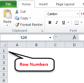
- As we can see in the above screenshot that each row can be identified by their row numbers like 1, 2, 3 etc.
- Whereas we can find the column in excel, which can be identified by the column header like A, B, C. which will be shown normally in all excel sheets, which are shown below.
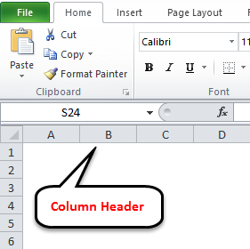
- In Excel, each column is named by its header, which shows the column header horizontally at the top of the excel sheet.
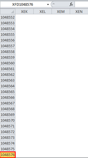
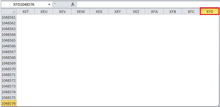
In Microsoft Excel 2010 and the latest version, we have row numbers ranging from 1 to 1048576 in 1048576, whereas the column ranges from A to XFD in a total of 16384 columns which is shown in the below screenshot.
Rows in excel range from 1 to 1048576, which is highlighted in red mark
The column in excel ranges from A to XFD, which is highlighted in red mark.
Rows and Column Navigation in excel
In this example, we will see how to navigate rows and columns with the below examples.
We can find the last row of excel by using the keyboard shortcut key CTRL+DOWN NAVIGATION ARROW KEY, or else we can use the vertical scrollbars to go to the end of the row.
We can find the last column of excel by using the CTRL+RIGHT NAVIGATION ARROW KEY, or else we can use the horizontal scrollbars to go to the end of the column.
How to Select Rows and Column in excel?
In this example, we will learn how to select the rows and columns in excel.
You can download this Rows and Column Excel Template here – Rows and Column Excel Template
Rows and Column in Excel – Example#1
Normally, when we open a workbook, we can see that sheet contains tabular rows and columns where each row is specified by their row number and column specified by their column header.
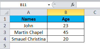
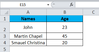
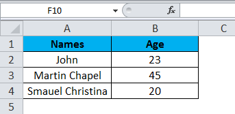
Consider the below example, which has some data in an excel sheet. Here we will see how to select the rows and columns.
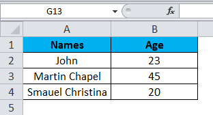
In the above screenshot, we can see that names and age column have their own header name A and B, and each row has its own row number.
In excel, each time when we select a row or column, “Name Box” will display the specific row number and column name, which is shown in the below screenshot.
In this example, we will select the Names and Age, and let’s see how the rows and column header is getting displayed.
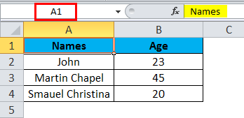
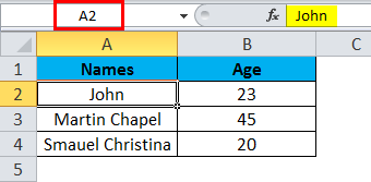
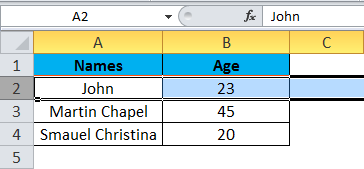
Step 1 – First, select the cell Name John.
Step 2 – Once you select the cell name, John, we will get the row number and column name as A2 in the name box, which means that we have selected A column second row as A2, shown below screenshot with yellow highlighted.
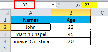
Step 3 – Now select cell 23, where it will show the selected cell is B2 which is shown in the below screenshot with yellow highlighted.
Step 4 – Now select all the names and columns to show that we have 4 rows and 2 columns shown in the below screenshot.
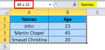
In this way, we can identify the row number and column name by selecting each cell in excel.
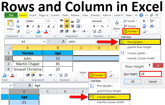
Example#2 – Changing Row and Column Size
This example shows how to change the row and column size by using the following examples.
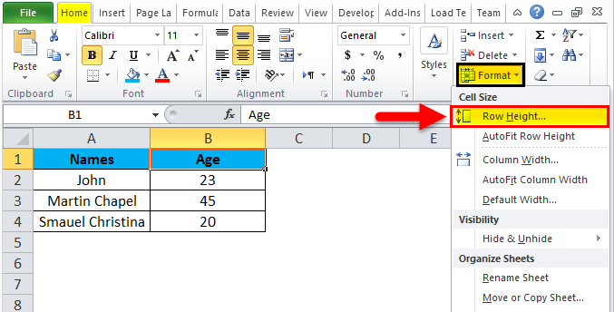
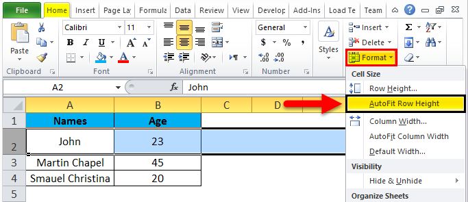
Excel row and column width size can be modified by using the format option in the HOME menu, which is shown below.
Using the format menu, we can change the row and column width where we have the list option, which are as follows:
- ROW HEIGHT– This is used to adjust the row height.
- AUTOFIT ROW HEIGHT– This will automatically adjust the row height.
- COLUMN WIDTH – This is used to adjust column width.
- AUTOFIT COLUMN WIDTH– This will automatically adjust the column width.
Let’s consider the below example to change the row and column width. Follow the below steps.
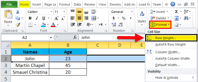
Step 1 – First, select the second row as shown in the below screenshot.
Step 2 – Go to the Format menu and click on ROW HEIGHT, as shown below.
Step 3 – Once we select the ROW HEIGHT, we will get the below dialog box to change the height of the row.
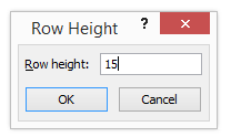
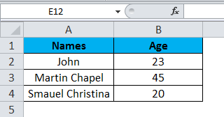
Step 4 – Now increase the row height to 25 so that the selected row height will get increased, as shown in the below screenshot.

We can see that row height has been increased when compared to the previous one; alternatively, we can change the row height by using the mouse.
Step 5 – Now go to the second option in the format list called AUTOFIT ROW HEIGHT, which will automatically reset the row to its original height.
Step 6 – Select the same row and go to the Format menu.
Step 7 – Now select the “AutoFit Row Height” as shown below.
Once we click on the “AutoFit Row Height” option, the row height will reset to the original position, shown below.
Adjusting Column Width
We can adjust the column width in the same way by using the format option.
Step 1 – First, click on the cell B cell as shown below.
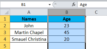
Step 2 – Now go to the Format menu and click on column width as shown in the below screenshot.
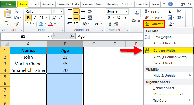
Once we click on the Column width, we will get the below dialog box to increase the column width, as shown below.
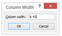
Step 3 – Now increase the column width by 15 to increase the selected column width.
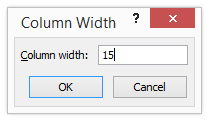
In the above screenshot, we can see that column width has been increased; alternatively, we can adjust the column width by using the mouse where if we place the mouse cursor, we will get the + plus mark sign near to the column.
Step 4 – Now click on the next option called “AutoFit Column width”. So that the selected column will get reset to its original size, which is shown below.
Things to Remember
- In excel, we can delete and insert multiple rows and columns.
- We can hide the specific row and columns using the hide option.
- Row and column cells can be protected by locking the specific cells.
Recommended Articles
This has been a guide to Rows and Columns in Excel. Here we also discuss Rows and Columns in Excel along with practical examples and downloadable excel template. You can also go through our other suggested articles –
- Excel Compare Two Columns
- Unhide Columns in Excel
- Sort Columns in Excel
- Excel Columns to Rows
Working with Excel means working with cells and ranges in the rows and columns in it.
And if you work with large datasets, selecting entire rows and columns is quite a common task.
Just like with most things in Excel, there is more than one way to select a column or row in Excel.
In this tutorial, I will show you how to select a column or row using a simple shortcut, as well as some other easy methods.
I will also show you how to do this when you’re working with an Excel table or Pivot Table.
So let’s get started!
Select Entire Column/Row Using Keyboard Shortcut
Let’s start with the keyboard shortcut.
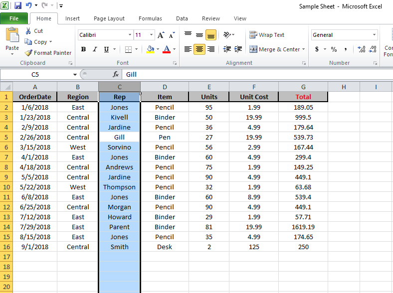
Suppose you have a dataset as shown below and you want to select an entire column (say column C).

The first thing to do is select any cell in Column C.
Once you have any cell in column C selected, use the below keyboard shortcut:
CONTROL + SPACE
Hold the Control key and then press the spacebar key on your keyboard
In case you’re using Excel on Mac, use COMMAND + SPACE
The above shortcut would instantly select the entire column (as you will see it gets highlighted in gray – indicating that it’s selected)

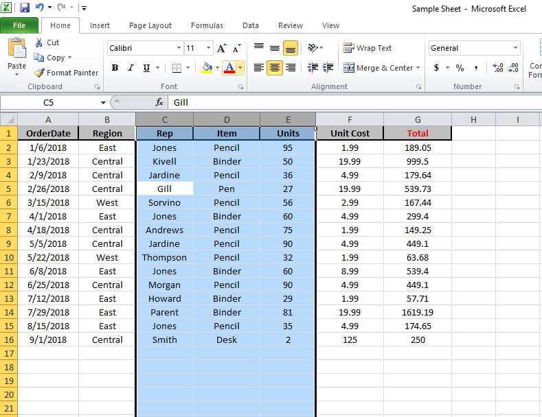
You can use the same shortcut to select multiple contiguous columns as well. For example, suppose you want to select both columns C and D.
To do this, select two adjacent cells (one in column C and one in Column D) and then use the same keyboard shortcut.
Selecting the Entire Row
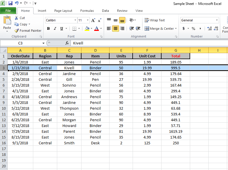
If you want to select the entire row, select any cell in the row that you want to be selected and then use the below keyboard shortcut
SHIFT + SPACE
Hold the Shift key and then press the Spacebar key.
You will again see that it gets selected and highlighted in gray.

In case you want to select multiple contiguous rows, select multiple adjacent cells in the same column and then use the keyboard shortcut.
Also read: Select Every Other Row in Excel
Select Entire Column (or Multiple Columns) Using Mouse
I have a feeling you may already know this method, but let me cover it anyway (it will be short).
Select One Column (or Row)
If you want to select an entire column (say column D), hover the cursor over the column headers (where it says D). You will notice that the cursor changes to a black downward-pointing arrow.
Now, click the left mouse key.
Doing this will select the entire column D.

Similarly, if you want to select the entire row, click on the row number (in the row header on the left)
Select Multiple Contiguous Columns (or Rows)
Suppose you want to select multiple columns that are next to each other (say column D, E, and F)
Follow the below steps to do this:
- Place the cursor on the left most column header of column D
- Press the left mouse key and keep it pressed
- With the left key pressed, drag the mouse to also cover column E and F
The above steps would automatically select all the columns in between the first and the last selected column.

And the same way, you can also select multiple contiguous rows.
Select Multiple Non-Contiguous Columns (or Rows)
This is the most common scenario where you need to select multiple columns that are not next to each other (say column D, and F).
Below are the steps to do this:
- Place the cursor at the column heading of one of the columns (say column D in this case)
- Click the mouse left key to select the column
- Press and hold the Control key
- With the Control key pressed, select all the other columns you want to select

You can do the same with rows as well.
Select Entire Column (or Multiple Columns) Using Name Box
Use this method when you want to:
- Select a far-off row or column
- Select multiple contiguous or non-contiguos rows/columns
Name box is a small box that is left of the formula bar.

While the main purpose of the Name Box is to quickly name a cell or range of cells, you can also use it to quickly select any column (or row).
For example, if you want to select the entire column D, enter the following in the name box and hit enter:
D:D
Similarly, if you want to select multiple columns (say D, E, and F), enter the following in the name box:
D:F
And that’s not it!
If you want to select multiple columns that are not adjacent, say D, H, and I, you can enter the below:
D:D,H:H,I:I
When I used to work as a financial analyst years ago, I found this trick extremely useful. It allowed me to quickly select columns and format them at once, or delete/hide these columns in one go.
The Named Range Trick
Let me also show you another wonderful trick.
Suppose you’re working in a workbook where you may often have a need to select far-off columns (say column B, D, and G).
Instead of doing it one by one or entering it manually in the Name Box, here is what you can do – create a named range that refers to the columns you want to select.
Once created, you can simply enter the named range name in the Name box (or select it from the drop-down)
Below are the steps to create a named range for specific columns:
- Select the columns for which you want to create the named range (hold the Control key and then select the columns one-by-one)
- Enter the name you want to give to the selection in the Name Box (no spaces allowed in the name). In this example, I will use the name SalesData

- Hit Enter
Once this is done, you have created a named range in Excel that now refers to the columns you selected (B, D, and G in my example).
And now it’s time for magic.
If you want to quickly select the columns B, D, and G, just enter the name in the Name box and hit enter (or click on the small drop-down icon at the end of the name box and select the name from the list).

Voila, all the columns would be selected.

This technique is useful if you may have a need to select the same columns multiple times in the same sheet.
You can use this technique to select rows as well as different ranges. For example, if you want to select two separate ranges in Excel, just follow the same steps (instead of selected columns, select the ranges and give them a name).
Select Column in an Excel Table
When working with Excel Tables, you may sometimes have a need to select an entire row or column in the table.
This means that you don’t want to select the entire column in the worksheet, but the entire column of the table.
Here is the trick to do this:
- Place the cursor on the header of the Excel table (note this is the header of the column in the Excel table, not the one that displays the column letter)
- You will notice that the cursor would chnage into a downward pointing black arrow

- Click the left mouse key
The above steps would select the entire column in the Excel Table (and not the full column).
And if you want to select multiple columns, hold the Control key and repeat the process for all the columns you want to select.
Also read: AutoSum in Excel (Shortcut)
Select Column in an Pivot Table
Just like the Excel table, you can also quickly select an entire row or column in a Pivot Table.
Suppose you have a Pivot Table as shown below and you want to select the Sales columns,
Below are the steps to do this:
- Place the cursor on the header of the Pivot table header that you want to select
- You will notice that the cursor would chnage into a downward pointing black arrow

- Click the left mouse key
These steps would select the Sales column. Similarly, if you want to select multiple columns, hold the Control key and then make the selection.
So these are some of the common ways you can use to select an entire column or an entire row in Excel.
I hope you found this tutorial useful!
Other Excel tutorials you may also like:
- Flip Data in Excel | Reverse Order of Data in Column/Row
- How to Lock Row Height & Column Width in Excel (Easy Trick)
- How to Delete All Hidden Rows and Columns in Excel
- 7 Easy Ways to Select Multiple Cells in Excel
- How to Insert Multiple Rows in Excel
- How to Copy and Paste Column in Excel? 3 Easy Ways!
- How to Multiply a Column by a Number in Excel
- Select Till End of Data in a Column in Excel (Shortcuts)
- How to Group Columns in Excel?
Bottom line: Learn some of my favorite keyboard shortcuts when working with rows and columns in Excel.
Skill level: Easy
Whether you are creating a simple list of names or building a complex financial model, you probably make a lot of changes to the rows and columns in the spreadsheet. Tasks like adding/deleting rows, adjusting column widths, and creating outline groups are very common when working with the grid.
This post contains some of my favorite shortcuts that will save you time every day.
I’ve also listed the equivalent shortcuts for the Mac version of Excel where available.
#1 – Select Entire Row or Column
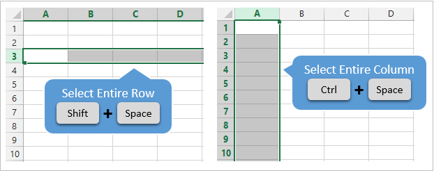
Shift+Space is the keyboard shortcut to select an entire row.
Ctrl+Space is the keyboard shortcut to select an entire column.
Mac Shortcuts: Same as above
The keyboard shortcuts by themselves don’t do much. However, they are the starting point for performing a lot of other actions where you first need to select the entire row or column. This includes tasks like deleting rows, grouping columns, etc.
These shortcuts also work for selecting the entire row or column inside an Excel Table.
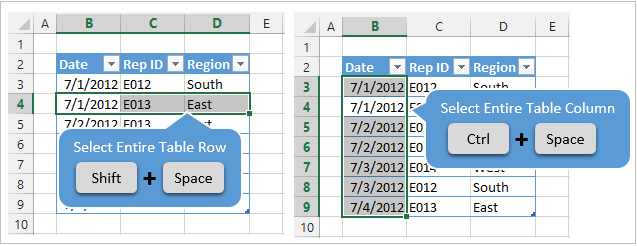
When you press the Shift+Space shortcut the first time it will select the entire row within the Table. Press Shift+Space a second time and it will select the entire row in the worksheet.
The same works for columns. Ctrl+Space will select the column of data in the Table. Pressing the keyboard shortcut a second time will include the column header of the Table in the selection. Pressing Ctrl+Space a third time will select the entire column in the worksheet.
You can select multiple rows or columns by holding Shift and pressing the Arrow Keys multiple times.
![]()
#2 – Insert or Delete Rows or Columns
There are a few ways to quickly delete rows and columns in Excel.
If you have the rows or columns selected, then the following keyboard shortcuts will quickly add or delete all selected rows or columns.
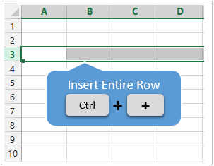
Ctrl++ (plus character) is the keyboard shortcut to insert rows or columns. If you are using a laptop keyboard you can press Ctrl+Shift+= (equal sign).
Mac Shortcut: Cmd++ or Cmd+Shift+
Ctrl+- (minus character) is the keyboard shortcut to delete rows or columns.
Mac Shortcut: Cmd+-
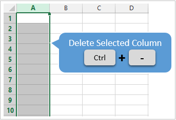
So for the above shortcuts to work you will first need to select the entire row or column, which can be done with the Shift+Space or Ctrl+Space shortcuts explained in #1.
If you do not have the entire row or column selected then you will be presented with the Insert or Delete Menus after pressing Ctrl++ or Ctrl+-.
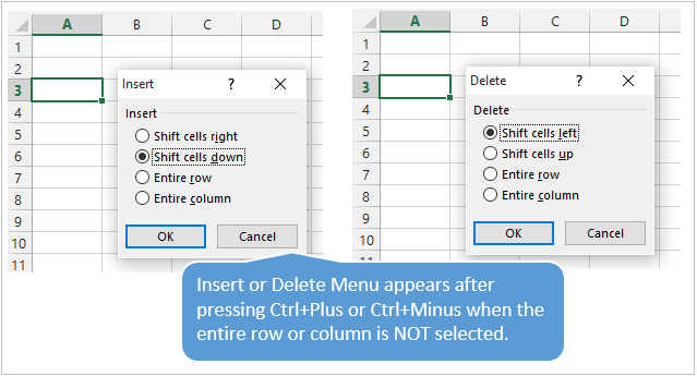
You can then press the up or down arrow keys to make your selection from the menu and hit Enter. For me it is easier to first select the entire row or column, then press Ctrl++ or Ctrl+-.
So, the entire keyboard shortcut to delete a column would be Ctrl+Space, Ctrl+-. You could also use the keyboard shortcut Alt+H+D+C to delete columns and Alt+H+D+R to delete rows. There are lots of ways to do a simple task… 🙂
#3 – AutoFit Column Width
There are also a lot of different ways to AutoFit column widths. AutoFit means that the width of the column will be adjusted to fit the contents of the cell.
You can use the mouse and double-click when you hover the cursor between columns when you see the resize column cursor.
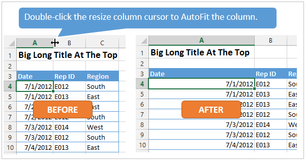
The problem with this is that you might just want to resize the column for the date in cell A4, instead of the big long title in cell A1. To accomplish this you can use the AutoFit Column Width button. It is located on the Home tab of the Ribbon in the Format menu.
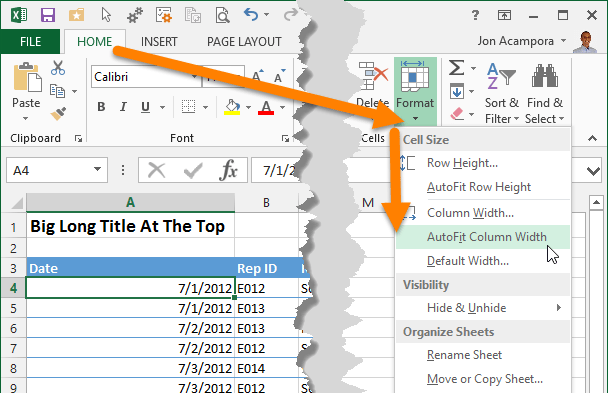
The AutoFit Column Width button bases the width of the column on the cells you have selected. In the image above I have cell A4 selected. So the column width will be adjusted to fit the contents of A4, as shown in the results below.
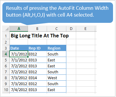
Alt,H,O,I is the keyboard shortcut for the AutoFit Column Width button. This is one I use a lot to get my reports looking shiny. 🙂
Alt,H,O,A is the keyboard shortcut to AutoFit Row Height. It doesn’t work exactly the same as column width, and will only adjust the row height to the tallest cell in the entire row.
Mac Shortcuts: None that I know of. The Mac version does not use the Alt key sequence which I believe is a limitation of the Mac OS.
#3.5 – Manually Adjust Row or Column Width
The column width or row height windows can be opened with keyboard shortcuts as well.
Alt,O,R,E is the keyboard shortcut to open the Row Height window.
Alt,O,C,W is the keyboard shortcut to open the Column Width window.
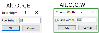
The row height or column width will be applied to the rows or columns of all the cells that are currently selected.
These are old shortcuts from Excel 2003, but they still work in the modern versions of Excel.
Mac Shortcuts: None that I know of. The Mac version does not use the Alt key sequence which I believe is a limitation of the Mac OS.
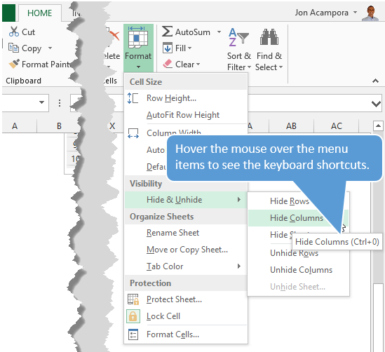
#4 – Hide or Unhide Rows or Columns
There are several dedicated keyboard shortcuts to hide and unhide rows and columns.
- Ctrl+9 to Hide Rows
- Ctrl+0 (zero) to Hide Columns
- Ctrl+Shift+( to Unhide Rows
- Ctrl+Shift+) to Unhide Columns – If this doesn’t work for you try Alt,O,C,U (old Excel 2003 shortcut that still works). You can also modify a Windows setting to prevent the conflict with this shortcut. See the comment from Pablo Baez on Oct 5, 2015 below for further instructions. Thanks Pablo! 🙂
Mac Shortcuts: Same as above
The buttons are also located on the Format menu on the Home tab of the Ribbon. You can hover over any of the items in the menu and the keyboard shortcut will display in the screentip (see screenshot below).
The trick with getting these shortcuts to work is to have the proper cells selected first.
To hide rows or columns you just need to select cells in the rows or columns you want to hide, then press the Ctrl+9 or Ctrl+Shift+( shortcut.
To unhide rows or columns you first need to select the cells that surround the rows or columns you want to unhide. In the screenshot below I want to unhide rows 3 & 4. I first select cell B2:B5, cells that surround or cover the hidden rows, then press Ctrl+Shift+( to unhide the rows.
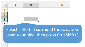
The same technique works to unhide columns.
#5 – Group or Ungroup Rows or Columns
Row and Column groupings are a great way to quickly hide and unhide columns and rows.
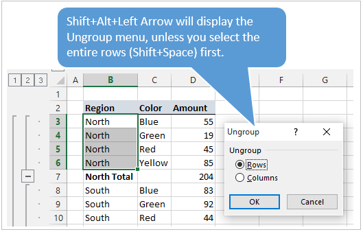
Shift+Alt+Right Arrow is the shortcut to group rows or columns.
Mac Shortcut: Cmd+Shift+K
Shift+Alt+Left Arrow is the shortcut to ungroup.
Mac Shortcut: Cmd+Shift+J
Again, the trick here is to select the entire rows or columns you want to group/ungroup first. Otherwise you will be presented with the Group or Ungroup menu.
Alt,A,U,C is the keyboard shortcut to remove all the row and columns groups on the sheet. This is the same as pressing the Clear Outline button on the Ungroup menu of the Data tab on the Ribbon.
*Bonus funny: At some point when using the group/ungroup shortcuts, you will accidentally press Ctrl+Alt+Right Arrow. This is a Windows shortcut that orientates the entire screen to the right. I call it “neck ache view”. To get it back to normal press Ctrl+Alt+Up Arrow.
If your co-worker or boss accidentally leaves their computer unlocked and you want to play a joke on them, press Ctrl+Alt+Down Arrow. This will turn their screen upside down. Don’t forget to record a video of their WTF reaction… 🙂
What Are Your Favorites?
There are a ton of keyboard shortcuts for working with rows and columns. The above are some of my favorites that I use everyday. What are some of your favorites? Please leave a comment below. Thanks! 🙂
In this article, we will learn how to select an entire column in excel and how to select whole row or a table using keyboard shortcut keys. While preparing reports and dashboard in Excel, it’s time-consuming to select an entire column using the mouse. These excel shortcuts are useful to save time and help you do your work faster using the keyboard shortcut keys. How to select row with the Excel shortcut?
Selecting cells is a very common function in Excel. It performs many tasks like addition, deletion and width adjustment of multiple rows and columns while applying the formula on data in Excel. Shortcut keys to select all rows and columns can provide an easier and quicker method of using MS Excel 2016. We have a data set here, let’s understand with the example.
How to Select Column in Excel Using Keyboard Shortcuts (CTRL+SPACE)
While navigating on an excel sheet with large data, excel column selection is very basic yet important task. Let’s see how easy is selecting columns in excel.
- Select any cell in any column.
- Press Ctrl + Space shortcut keys on the keyboard. The whole column will be highlighted in excel to show the selected column, as shown below in the picture. You can also say that this is a shortcut to highlight column in excel.
If you wish to select the adjacent columns with the selected column, use Shift + Left/Right arrow key(s) to select entire columns left or right of that column. You can go either way but can’t select both sides of column.
Let’s Select Entire Columns C to E
- To Select Column C:E, Select any cell of the 3rd column.
- Use Ctrl + Space shortcut keys from your keyboard to select column E (Leave the keys if the column is selected).
- Now use Shift + Right (twice) arrow keys to select columns D and E, simultaneously.
- You can select columns C:A by using shortcut Shift + Left (twice) arrow keys.
- You can select columns to the end of sheet using Ctrl+Shift + Left shortcut.
- To select to end of column from a cell, use excel shortcut Ctrl+Shift + Down arrow.
You can’t select columns A:E if you start from any column in between. I am repeating, you can only select entire columns in Excel from left or right of initial column.
How to Select Entire Row Using Keyboard Shortcuts in Excel (SHIFT+SPACE)
This command is used for selecting rows in excel. This is also a shortcut to highlight a row in excel.
- Select the cell in the row you wish to select.
- Press Shift+ Space key to select the row on the selected cell (release the keys, if the row is selected).
- If you wish to select the adjacent rows with the selected row, press Shift+ Up/down arrow key(s) to select the UP or DOWN to that row. You can go either way but can’t access both sides of it.
Selecting 3rd to 5th whole rows of the sheet can be done in two ways:
- Select any cell of the 3rd row, press Shift + Space key to select the row.
- Now use Shift + Down(twice) arrow key to select the 4th and the 5th row.
- Or you could go another way from 5th to 3rd row but you won’t be able to select 3rd and 5th row both, starting from the 4th row.

Select multiple rows and columns of a table with shortcut keys and perform your tasks efficiently.
Frequently Asked Question:
How to apply formula to entire column?
Easy, write a formula in the first cell of column and press CTRL + SPACE to select entire column and then CTRL+D to apply formula to entire column.
How to select all in excel?
To select all data press CTRL+A.
How to highlight a row in excel?
Just select any cell in the row you want to highlight and Press Shift+ Space.
How to select multiple cells in Excel mac?
Hold down the command key and scroll over the cells to select. If the cells are not adjacent then click on the cells while holding the command key.
Hope you understood how to select columns and rows with shortcuts in Excel. You can perform these tasks in 2013 and 2010. Explore more links on shortcut keys here. If you have any query, please mention in the comment box below. We will help you.
If you liked our blogs, share it with your friends on Facebook. And also you can follow us on Twitter and Facebook.
We would love to hear from you, do let us know how we can improve, complement or innovate our work and make it better for you. Write us at info@exceltip.com
What To Know
- To highlight rows: Shift+Space. Arrows Up or Down for additional rows.
- To select columns: Ctrl+Space. Arrows Left or Right for additional columns.
- To highlight every cell in the sheet: Ctrl+A
This article explains how to change column/row dimensions, hiding columns/rows, inserting new columns/rows, and applying cell formatting in Excel, using a series of convenient hotkeys. Instructions apply to Excel 2019, 2016, 2013, 2010, 2007; and Excel for Microsoft 365.
Select Entire Rows in a Worksheet
Use Shortcut Keys to Select Rows
-
Click on a worksheet cell in the row to be selected to make it the active cell.
-
Press and hold the Shift key on the keyboard.
-
Press and release the Spacebar key on the keyboard.
Shift+Spacebar
-
Release the Shift key.
-
All cells in the selected row are highlighted; including the row header.
Use Shortcut Keys to Select Additional Rows
-
Press and hold the Shift key on the keyboard.
-
Use the Up or Down arrow keys on the keyboard to select additional rows above or below the selected row.
-
Release the Shift key when you’ve selected all the rows.
Use the Mouse to Select Rows
-
Place the mouse pointer on the row number in the row header. The mouse pointer changes to a black arrow pointing to the right.
-
Click once with the left mouse button.
Use the Mouse to Select Additional Rows
-
Place the mouse pointer on the row number in the row header.
-
Click and hold the left mouse button.
-
Drag the mouse pointer up or down to select the desired number of rows.
Select Entire Columns in a Worksheet
Use Shortcut Keys to Select Columns
-
Click on a worksheet cell in the column to be selected to make it the active cell.
-
Press and hold the Ctrl key on the keyboard.
-
Press and release the Spacebar key on the keyboard.
Ctrl+Spacebar
-
Release the Ctrl key.
-
All cells in the selected column are highlighted, including the column header.
Use Shortcut Keys to Select Additional Columns
To select additional columns on either side of the selected column:
-
Press and hold the Shift key on the keyboard.
-
Use the Left or Right arrow keys on the keyboard to select additional columns on either side of the highlighted column.
Use the Mouse to Select Columns
-
Place the mouse pointer on the column letter in the column header. The mouse pointer changes to a black arrow pointing down.
-
Click once with the left mouse button.
Use the Mouse to Select Additional Columns
-
Place the mouse pointer on the column letter in the column header.
-
Click and hold the left mouse button.
-
Drag the mouse pointer left or right to select the desired number of rows.
Select All Cells in a Worksheet
Use Shortcut Keys to Select All Cells
-
Click on a blank area of a worksheet that contains no data in the surrounding cells.
-
Press and hold the Ctrl key on the keyboard.
-
Press and release the letter A key on the keyboard.
Ctrl+A
-
Release the Ctrl key.
Use ‘Select All’ to Select All Cells
If you prefer not to use the keyboard, use Select All to quickly select all cells in a worksheet.
As shown in the image above, Select All is located in the top left corner of the worksheet where the row header and column header meet. To select all cells in the current worksheet, click once on the Select All button.
Select All Cells in a Table
Depending on the way the data in a worksheet is formatted, using the shortcut keys above will select different amounts of data. If the active cell is located within a contiguous range of data:
- Press Ctrl+A to select all the cells containing data in the range.
If the data range has been formatted as a table and has a heading row that contains drop-down menus:
- Press Ctrl+A a second time to select the heading row.
The selected area can then be extended to include all cells in a worksheet.
- Press Ctrl+A a third time to select the entire worksheet.
Select Multiple Worksheets
Not only is it possible to move between sheets in a workbook using a keyboard shortcut, but you can also select multiple adjacent sheets with a keyboard shortcut as well. Simply add the Shift key to the key combinations above.
To select pages to the left:
Ctrl+Shift+PgUp
To select pages to the right:
Ctrl+Shift+PgDn
Selecte Multiple Sheets
Using the mouse along with keyboard keys has one advantage over using just the keyboard. It allows you to select non-adjacent sheets as well as adjacent ones.
Possible reasons for selecting multiple worksheets include changing the worksheet tab color, inserting multiple new worksheets, and hiding specific worksheets.
Select Multiple Adjacent Sheets
-
Click on one sheet tab to select it.
-
Press and hold the Shift key on the keyboard.
-
Click on additional adjacent sheet tabs to highlight them.
Select Multiple Non-Adjacent Sheets
-
Click one sheet tab to select it.
-
Press and hold the Ctrl key on the keyboard.
-
Click on additional sheet tabs to highlight them.
FAQ
-
How do you merge cells in Excel?
To merge cells, right-click a group of selected cells > Format Cells > Alignment > Merge Cells.
-
How do you lock cells in Excel?
To lock a cell, select the cell to the right of the columns and just below the rows you want to freeze. Select the View tab > Freeze Panes > Freeze Panes.
Thanks for letting us know!
Get the Latest Tech News Delivered Every Day
Subscribe
Transcript
In this lesson, we’ll look at how to select entire rows and columns.
Selecting columns and rows is handy when you want to move information around, delete information, or when you want to copy a row or column.
Let’s take a look.
To select a column in Excel, just click the letter in the column heading.
You’ll see Excel immediately select the entire column.
If you want to select more than one column, and the columns are together, just click a column letter and drag to expand your selection.
If you want to select more than one column, and the columns are not next to one another, hold down the control key before you click. By holding down the control key, you can add as many columns to your selection as you like.
Rows work the same way as columns. To select a row, click the row number.
Like columns, you can click and drag to select more than one row at a time as long as the rows are together.
You can also hold down the control key to add rows that are not together to your selection.
Using the control key, you can even select a combination of rows and columns.

Author![]()
Dave Bruns
Hi — I’m Dave Bruns, and I run Exceljet with my wife, Lisa. Our goal is to help you work faster in Excel. We create short videos, and clear examples of formulas, functions, pivot tables, conditional formatting, and charts.