Select by color excel

Do you need to organize an Excel sheet by its cell color?

You often use color in a table to indicate related data. A good example would be a table of consumers who each have a favorite vegetable.

You might want to color the cell to match the color of their vegetable. You could then sort the table by color so that all vegetables of the same color appear together!

This post uses will show you different ways to sort by color in Excel.

Sort by Color from the Data Tab

The general steps of any sort are to select the data you need sorted and then specify the sort details.

Follow these steps to sort by color using the Data tab.

1. Select the cells you need to be sorted.

You can select either a single cell or a range within your table. Excel will try to guess what cells you want to be sorted if you select anything less than the full table.

1. Go to the Data tab.
2. Select the Sort command.

Select Expand the selection and click Sort… to sort the entire table. You will only get this prompt if Excel thinks you selected a partial table range.

By default, Excel assumes your topmost table row is a header. This example table has a header so ensure My data has headers is checked. Excel will exclude that row from sorting.

1. Select your column in the Sort by dropdown.
2. Select the Cell Color in the Sort On dropdown.
3. Select green in the Order dropdown and ensure On Top is selected so that green cells will appear first.

1. Click Add Level and select your column again in the new Sort by dropdown.
2. Select Cell Color again in the new Sort On dropdown.
3. This time select yellow in the Order dropdown so that yellow cells appear after green cells.

1. Repeat the process to add any other colors you want to sort.
2. Click OK when done.

💡 Tip: The order the rules appear in the Sort menu will be the order in which the colors are sorted. You can use the up and down arrow at the top of the menu to re-order the colors as needed.

Observe how your entire table gets sorted by green, yellow, and red in that order!

Sort by Color from Filter Toggles

You may already be using filter toggles in your table for reasons other than sorting. There is a sorting option on these toggles as well.

Follow these steps to apply the sort by color option from the filter toggles.

Ensure filter toggles are on by first selecting your table header.

Under the Data tab ensure the Filter option is toggled on.

Select the filter toggle of your colored cells column header.

Select the Sort by Color option and then choose the color to sort by. The selected color will appear at the top of the sorted data.

The Custom Sort selection is available if you want to sort by more than one color.

See how your whole table is now sorted with green cells on top! Notice too this basic sort leaves your other colors unsorted.

Sort by Color from the Right Click Menu

The right-click menu offers a quick way to access common Excel features like sorting.

These steps will allow you to sort by color with the right click menu.

1. Right-click on a cell whose color you want to sort by.

1. Select the Sort option.

1. Select the Put Selected Cell Color On Top option from the submenu.

Note a more complex sort is available with the Custom Sort option.

Your table now gets re-sorted so that all your green cells appear at the top! Be aware that this type of sort leaves your cells of other colors unsorted.

Sort by Color with VBA

VBA is available in the Desktop versions of Excel and can be used to automate tasks like sorting. You can write VBA code to sort by color for any currently selected range!

Follow these steps to get started with VBA.

Select the Developer tab and select the Visual Basic command or press Alt + F11. You might need to show the Developer tab if it’s hidden from the ribbon.

Select the Insert menu followed by the Module option.

Sub SortByColor()

Dim ws As Worksheet
Dim tbl As Range
Dim col As Range

Set ws = ActiveSheet
Set tbl = ws.UsedRange
Set col = Intersect(Selection.EntireColumn, tbl)

With ws.Sort
    .SortFields.Clear
    
    .SortFields.Add(col, _
        xlSortOnCellColor).SortOnValue.Color = vbGreen
    .SortFields.Add(col, _
        xlSortOnCellColor).SortOnValue.Color = vbYellow
    .SortFields.Add(col, _
        xlSortOnCellColor).SortOnValue.Color = vbRed
    
    .SetRange tbl
    .Header = xlYes
    .Apply
End With

End Sub

Double-click the new module and paste the above code into that module.

The code takes all the content of your active sheet as your table. Your active cell indicates the column of colors to sort.

The code first clears any previous sorting. The top-to-bottom sort priority is specified as green, yellow, and red. The code tells Excel to treat the top table row as a header and then applies the sort.

To run a the code you can select a cell within your colored column.

Go to the View tab and select Macros.

This will open the Macro menu where you can see all your available macros. Select your SortByColor macro and click the Run button.

Your table is now sorted by color!

Sort by Color with Office Scripts

Office Scripts is an scripting language that used to be only available in the online version of Excel under Microsoft 365 Business Plans. It has recently expanded into the beta channel of Desktop Excel as well.

You can sort by color using Office Scripts by following these steps.

Open your Excel workbook of table data.

Go to the Automate tab and select New Script.

If you don’t see the Automate tab, then your version of Excel might not support Office Scripts or you might need to enable this feature from the admin panel of your Microsoft 365 account.

function main(workbook: ExcelScript.Workbook) {

let ws = workbook.getActiveWorksheet();
let tbl = ws.getUsedRange();

let green: ExcelScript.SortField = {ascending: true, color: "00ff00", key: 1, sortOn: ExcelScript.SortOn.cellColor};

let yellow: ExcelScript.SortField = {ascending: true, color: "ffff00", key: 1, sortOn: ExcelScript.SortOn.cellColor};

let red: ExcelScript.SortField = { ascending: true, color: "ff0000", key: 1, sortOn: ExcelScript.SortOn.cellColor};

let hasHeaders = true;

tbl.getSort().apply([green, yellow, red], false, hasHeaders);

}

Paste the above script into the Code Editor pane.

The script assumes your table is the only content on the active sheet.

The green, yellow, and red colors are assumed to be in the second column by specifying the key as 1.

The 00ff00, ffff00, and ff0000 values are the hex code representations of each color. Setting hasHeaders to true excludes your table header from sorting.

The line tbl.getSort().apply does the sort with green, yellow, and red sorted in that order.

Try your code by selecting anywhere in your sheet and clicking the Run button on the code editor.

You immediately see the results of your color sort!

Conclusions

This post described to you how to sort by color in several different ways.

The conventional Data tab method lets you do a comprehensive sort using the Sort menu options.

You can do a quick one-color sort by going through the filter toggle or right-click menu. Be aware a multi-color sort is only possible through the Custom Sort option.

You can always implement VBA code if you’ll be repeatedly re-sorting your data. This goes for Office Scripts as well with supported licensing. Office Scripts is an expanding presence in Excel and is a good route to take for automating your sorting!

Have you ever needed to sort by cell color in Excel? How did you get this done? Let me know in the comments below!

Выделение ячеек в Excel по значению и по цвету

Найдите ячейки по вашим критериям

Используя этот простой инструмент для Excel, вы можете находить ячейки с одинаковыми данными, а также ячейки, содержащие формулы, комментарии, изображения или условные форматы. Вы также можете выделить уникальные записи и пустые ячейки, выбрать текстовые значения, числа или даты, соответствующие определенным критериям.

• 60-дневная безусловная гарантия возврата денег

• Бесплатные обновления на 2 года

• Бесплатная и бессрочная техническая поддержка

С помощью инструмента Select by Value & Color вы сможете:

Выделить все ячейки с одинаковым значением

Выберите интересующую вас ячейку и затем выделите все остальные ячейки, содержащие то же значение.

Выделить ячейки с числами и датами по различным условиям

Найдите числовые значения, которые равны или не равны, больше или меньше указанного вами числа; в пределах или за пределами определенного диапазона; минимальное, максимальное или уникальные.

Найти специальные ячейки

Ищите ячейки с константами или формулами, которые содержат текст, числа, логические значения или ошибки.

Найти ячейки с определенной заливкой или цветом шрифта

Выделите все ячейки, которые имеют тот же цвет фона или шрифта, что и выбранная ячейка.

Выделить текстовые ячейки по самым разным шаблонам

Найдите текстовые значения, которые начинаются, заканчиваются или содержат определенные символы; точно соответствует или не совпадает с вашим текстом, уникальными данными и многим другим.

Выбрать ячейки определенного типа

Выделите все ячейки с комментариями, константами, формулами, объектами, условными форматами или просто пустые.

Приложение Ultimate Suite уже используют

Что такое инструмент «Select by Value/Color» и зачем он мне нужен?

Речь идет не только о поиске ячеек по цвету и значению. Этот инструмент предлагает много различных вариантов для быстрого выделения ячеек в соответствии с вашими критериями. 

С помощью надстройки вы можете:

• Найти ячейки по цвету шрифта выбранной в данный момент ячейки.
• Выделить все ячейки тем же цветом фона, что и выбранная ячейка.
• Найдите ячейки с теми же данными, что и выбранная ячейка.
• Выделите ячейки, содержащие комментарии, значения, формулы, пробелы, объекты, условные форматы или просто пустые.

Кроме того, вы можете выбрать числа, даты или текстовые ячейки, которые:

• Больше или меньше указанного значения
• Равны или не равны заданному значению
• В пределах или за пределами определенного диапазона
• Текстовые строки, начинающиеся или заканчивающиеся определенными символами
• Текст, содержащий или не содержащий указанные символы
• Максимальные или минимальные значения
• Уникальные данные

Как найти одинаковые данные с помощью этой утилиты?

Выберите любую ячейку, содержащую данные, которые вы ищете, и выберите «Все ячейки с одинаковым значением» (All cells with the same value). Инструмент выделит все ячейки, содержащие те же данные, что и в выбранной ячейке.

Мне нужно выделить все ячейки с числами больше 100. Как я могу это сделать?

Это можно сделать с помощью опции «Выбрать по значению» (Select by Value). Укажите свой диапазон поиска и отметьте «Числа» (Numbers). Выберите пункт «Выбрать ячейки которые больше» (Select cells that are greater), введите 100 в соответствующее поле и нажмите «Выбрать» . Все ячейки, содержащие числа больше 100, будут выделены.

Могу ли я выделить все ячейки с условным форматированием?

Для этого используйте операцию Select Special Cells. Выделите диапазон и нажмите Выбрать ячейки, содержащие условные форматы (Select cells containing conditional formats). Нажмите кнопку «Выбрать» и просмотрите все ячейки текущего листа с выделенным условным форматированием.

Как найти в Excel ячейки, содержащие изображения?

Опция Select Special Cells поможет. Выберите Выбрать ячейки, содержащие объекты (Select cells containing objects), и все ячейки с изображениями будут найдены.

Может ли эта утилита помочь мне найти даты, попадающие в определенный диапазон?

Да, программа предлагает такую ​​возможность. Выберите свою область поиска и запустите надстройку Select by Value. Отметьте пункт «Даты» (Date). Затем выберите «Выбрать ячейки, которые находятся в диапазоне» (Select cells that are in the range) , определите этот диапазон и нажмите «Выбрать» .

Таким же образом вы можете найти даты, выходящие за пределы вашего диапазона, и даты, которые больше или меньше определенных дат.

Скачать  Ultimate Suite

Посмотреть все комментарии

Создатели Excel решили, начиная от 2007-ой версии ввести возможность сортировки данных по цвету. Для этого послужило поводом большая потребность пользователей предыдущих версий, упорядочивать данные в такой способ. Раньше реализовать сортировку данных относительно цвета можно было только с помощью создания макроса VBA. Создавалась пользовательская функция и вводилась как формула под соответствующим столбцом, по которому нужно было выполнить сортировку. Теперь такие задачи можно выполнять значительно проще и эффективнее.

Сортировка по цвету ячеек

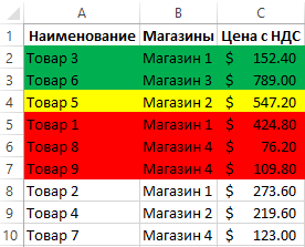
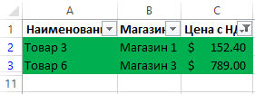
Пример данных, которые необходимо отсортировать относительно цвета заливки ячеек изображен ниже на рисунке:

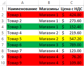
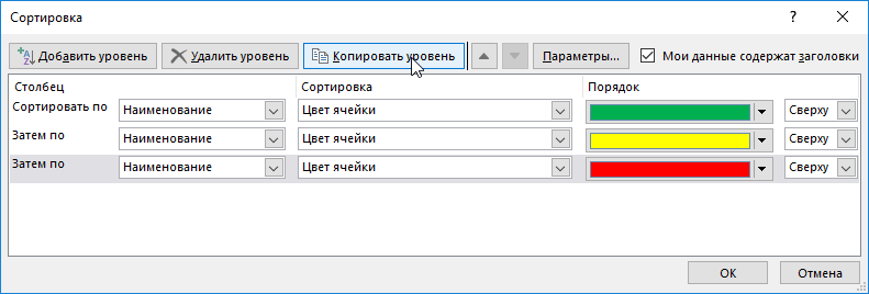
Чтобы расположить строки в последовательности: зеленый, желтый, красный, а потом без цвета – выполним следующий ряд действий:

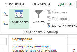
1. Щелкните на любую ячейку в области диапазона данных и выберите инструмент: «ДАННЫЕ»-«Сортировка и фильтр»-«Сортировка».



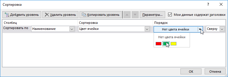
2. Убедитесь, что отмечена галочкой опция «Мои данные содержат заголовки», а после чего из первого выпадающего списка выберите значение «Наименование». В секции «Сортировка» выберите опцию «Цвет ячейки». В секции «Порядок» раскройте выпадающее меню «Нет цвета» и нажмите на кнопку зеленого квадратика.



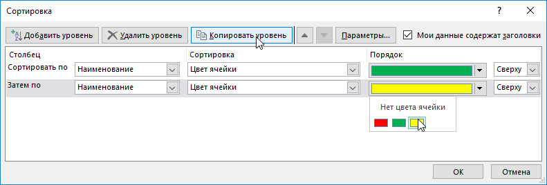
3. Нажмите на кнопку «Копировать уровень» и в этот раз укажите желтый цвет в секции «Порядок».



4. Аналогичным способом устанавливаем новое условие для сортировки относительно красного цвета заливки ячеек. И нажмите на кнопку ОК.

Ожидаемый результат изображен ниже на рисунке:

Аналогичным способом можно сортировать данные по цвету шрифта или типу значка которые содержат ячейки. Для этого достаточно только указать соответствующий критерий в секции «Сортировка» диалогового окна настройки условий.



Фильтр по цвету ячеек

Аналогично по отношению к сортировке, функционирует фильтр по цвету. Чтобы разобраться с принципом его действия воспользуемся тем же диапазоном данных, что и в предыдущем примере. Для этого:

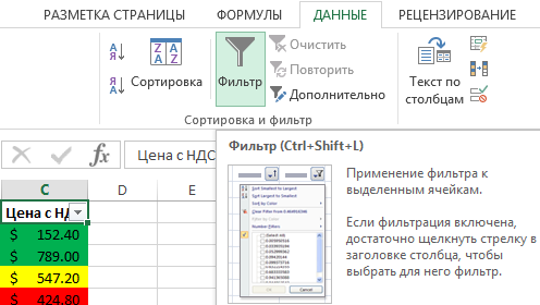
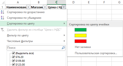
1. Перейдите на любую ячейку диапазона и воспользуйтесь инструментом: «ДАННЫЕ»-«Сортировка и фильтр»-«Фильтр».



2. Раскройте одно из выпадающих меню, которые появились в заголовках столбцов таблицы и наведите курсор мышки на опцию «Фильтр по цвету».



3. Из всплывающего подменю выберите зеленый цвет.

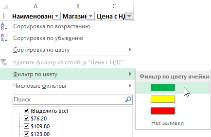
В результате отфильтруються данные и будут отображаться только те, которые содержать ячейки с зеленым цветом заливки:

Обратите внимание! В режиме автофильтра выпадающие меню так же содержит опцию «Сортировка по цвету»:

Как всегда, Excel нам предоставляет несколько путей для решения одних и тех же задач. Пользователь выбирает для себя самый оптимальный путь, плюс необходимые инструменты всегда под рукой.

Excel has a lot of options when it comes to sorting data.

And one of those options allows you to sort your data based on the color of the cell.

For example, in the below dataset, you can sort by color to get the names of all the students who scored above 80 together at the top and all the students who scored less than 35 together at the bottom.

With the sorting feature in Excel, you can sort based on the color in the cell.

In this tutorial, I will show you different scenarios where you can sort by color and the exact steps you need to do this.

Note that in this tutorial, I have taken examples where I am sorting based on numeric values. However, these methods work perfectly well even if you have text or dates instead of numbers.

Sort Based on a Single Color

If you only have a single color in your dataset, you can easily sort it based on it.

Below is a dataset where all the students who have scored more than 80 have been highlighted in green.

Here are the steps to sort by the color of the cells:

1. Select the entire dataset (A1:B11 in this example)
2. Click the Data tab
3. Click on the ‘Sort’ option. This will open the Sort dialog box.
4. In the Sort dialog box, make sure ‘My Data has headers’ is selected. In case your data doesn’t have headers, you can keep this option unchecked.
5. Click the ‘Sort By’ drop down and select ‘Marks’. This is the column based on which we want the data to be sorted.
6. In the ‘Sort On’ drop down, click on Cell Color.
7. In the ‘Order’ drop-down, select the color based on which you want to sort the data. Since there is only one color in our dataset, it only shows one color (green)
8. In the second drop-down in Order, select On-top. This is the place where you specify whether you want all the colored cells at the top of the dataset or at the bottom.
9. Click OK.

The above steps would give you a dataset as shown below.

Keyboard Shortcut to Open the Sort Dialog box – ALT A S S (hold the ALT key then press A S S keys one by one)

Note that sorting based on color only rearranges the cells to bring together all the cells with the same color together. Rest of the cells remain as is.

This method works for cells that you have highlighted manually (by giving it a background color) as well as the ones where the cell color is because of conditional formatting rules.

Sort Based on Multiple Colors

In the above example, we only had cells with one color that needed to be sorted.

And you can use the same methodology to sort when you have cells with multiple colors.

For example, suppose you have a dataset as shown below where all the cell where the marks are more than 80 are in green color and the ones where marks are less than 35 are in red color.

And you want to sort this data so that you have all the cells with green at the top and all the ones with red at the bottom.

Below are the steps to sort by multiple colors in Excel:

1. Select the entire dataset (A1:B11 in this example)
2. Click the Data tab.
3. Click on the Sort option. This will open the Sort dialog box.
4. In the Sort dialog box, make sure ‘My Data has headers’ is selected. In case your data doesn’t have headers, you can keep this option unchecked.
5. Click the ‘Sort By’ drop down and select ‘Marks’. This is the column based on which we want the data to be sorted.
6. In the ‘Sort On’ drop down, click on Cell Color.
7. In the ‘Order’ drop-down, select the first color based on which you want to sort the data. It will show all the colors that are there in the dataset. Select green.
8. In the second drop-down in Order, select On-top.
9. Click on Add Level button. This is done to add another condition of sorting (as we want to sort based on two colors). Clicking this button would add another set of sorting options.
10. Click the ‘Then by’ drop-down and select ‘Marks’
11. In the ‘Sort On’ drop down, click on Cell Color.
12. In the ‘Order’ drop-down, select the second color based on which you want to sort the data. It will show all the colors that are there in the dataset. Select Red.
13. In the second drop-down in Order, select On-Bottom.
14. Click OK

The above steps would sort the data with all the green at the top and all the reds at the bottom.

Clarification: Sorting by color works with numbers as well as text data. You may be thinking that you can achieve the results shown above by just sorting the data based on the values. While, this will work in this specific scenario, imagine you have a huge list of clients/customers/products that you have manually highlighted. In that case, there is no numeric value, but you can still sort based on the color of the cells.

Sort Based on Font Color

Another amazing thing about sorting in Excel is that you can also sort by font color in the cells.

While this is not as common as getting data where cells are colored, this is still something a lot of people do. After all, it only takes one click to change the font color.

Suppose you have a dataset as shown below and you want to sort this data to get all the cells with the red color together.

Below are the steps to sort by font color in Excel:

1. Select the entire dataset (A1:B11 in this example)
2. Click the Data tab
3. Click on the Sort option. This will open the Sort dialog box.
4. In the Sort dialog box, make sure ‘My Data has headers’ is selected. In case your data doesn’t have headers, you can keep this option unchecked.
5. Click the Sort By drop down and select ‘Marks’. This is the column based on which we want the data to be sorted.
6. In the ‘Sort On’ drop down, click on Font Color.
7. In the ‘Order’ drop-down, select the color based on which you want to sort the data. Since there is only one color in our dataset, it only shows one color (red)
8. In the second drop-down in Order, select On-top. This is the place where you specify whether you want all the colored cells at the top of the dataset or at the bottom.
9. Click OK.

The above steps would sort the data with all the cells with the font in red color at the top.

Sort Based on Conditional Formatting Icons

Conditional formatting allows you to add a layer of visual icons that can make your data or your reports/dashboards look a lot better and easy to read.

If you have such data with conditional formatting icons, you can also sort this data based on the icons

Suppose you have a dataset as shown below:

Below are the steps to sort by conditional formatting icons:

1. Select the entire dataset (A1:B11 in this example)
2. Click the Data tab
3. Click on the Sort option. This will open the Sort dialog box.
4. In the Sort dialog box, make sure ‘My Data has headers’ is selected. In case your data doesn’t have headers, you can keep this option unchecked.
5. Click the ‘Sort By’ drop down and select ‘Marks’. This is the column based on which we want the data to be sorted.
6. In the ‘Sort On’ drop down, click on ‘Conditional Formatting Icon’.
7. In the ‘Order’ drop-down, select the icon based on which you want to sort the data. It will show all the icons that are there in the dataset. Select the green one first.
8. In the second drop-down in Order, select On-top.
9. Click on Add Level button. This is done to add another condition of sorting (as we want to sort based on three icons). Clicking this button would add another set of sorting options.
10. Click the ‘Then by’ drop-down and select ‘Marks’
11. In the ‘Sort On’ drop down, click on ‘Conditional Formatting Icons’.
12. In the ‘Order’ drop-down, select the second icon based on which you want to sort the data. It will show all the icons that are there in the dataset. Select yellow.
13. In the second drop-down in Order, select On-Top.
14. Click on Add Level button. This is done to add another condition of sorting. Clicking this button would add another set of sorting options.
15. Click the ‘Then by’ drop-down and select ‘Marks’
16. In the ‘Sort On’ drop down, click on ‘Conditional Formatting Icons’.
17. In the ‘Order’ drop-down, select the third icon based on which you want to sort the data. It will show all the icons that are there in the dataset. Select Red.
18. In the second drop-down in Order, select On-Top.
19. Click OK.

The above steps would sort the data set and give you all the similar icons together.

Note that sorting will follow the order in which you have it in the sorting dialog box. For example, if all the icons are set to sort and show at the top, first all the cells with green icons would be shown as it’s at the top in our three conditions. Then the resulting data would have the yellow icons and then the red icons.

Not Losing the Original Order of the Data

When you sort the data, you lose the original order of the dataset.

In case you want to keep the original dataset as well, it’s best to create a copy of the data and then perform the sorting on the copied data.

Another technique to make sure you can get back the original data is to insert a column with row numbers.

Once you have this column added, use this when sorting the data.

In case you need the original data order back at a later stage, you can easily sort this data based in the columns with the numbers.

Interested in learning more about sorting data in Excel. Here is a massive give on how to sort in Excel that covers a lot of topics such as sorting by text/dates/numbers, sorting from left-to-right, sorting based on partial text, case sensitive sorting, multi-level sorting and much more.

You May Also Like the Following Excel Tutorials:

• Highlight Rows Based on a Cell Value in Excel
• How to Sort by Length in Excel?
• How to Sum by Color in Excel (Formula & VBA)
• How to Count Colored Cells in Excel
• Search and Highlight Data Using Conditional Formatting
• Multiple Level Data Sorting in Excel
• Sort Data in Excel using VBA
• How to Move Rows and Columns in Excel
• Highlight the Active Row and Column in Excel
• How to Undo Sort in Excel
• Filter By Color in Excel