
Содержание
- Select rows and columns in an Excel table
- Need more help?
- Select cell contents in Excel
- Select one or more cells
- Select one or more rows and columns
- Select table, list or worksheet
- Need more help?
- 7 Easy Ways to Select Multiple Cells in Excel
- Select Multiple Cells (that are all contiguous)
- Select Rows/Columns
- Select a Single Row/Column
- Select Multiple Rows/Columns
- Select Multiple Non-Adjacent Rows/Columns
- Select All the Cells in the Current Table/Data
- Select All the Cells in the Worksheet
- Select Multiple Non-Contiguous Cells
- Select Cells Using Name Box
- Select a Named Range
Select rows and columns in an Excel table
You can select cells and ranges in a table just like you would select them in a worksheet, but selecting table rows and columns is different from selecting worksheet rows and columns.
A table column with or without table headers
Click the top edge of the column header or the column in the table. The following selection arrow appears to indicate that clicking selects the column.

Note: Clicking the top edge once selects the table column data; clicking it twice selects the entire table column.
You can also click anywhere in the table column, and then press CTRL+SPACEBAR, or you can click the first cell in the table column, and then press CTRL+SHIFT+DOWN ARROW.
Note: Pressing CTRL+SPACEBAR once selects the table column data; pressing CTRL+SPACEBAR twice selects the entire table column.
Click the left border of the table row. The following selection arrow appears to indicate that clicking selects the row.

You can click the first cell in the table row, and then press CTRL+SHIFT+RIGHT ARROW.
All table rows and columns
Click the upper-left corner of the table. The following selection arrow appears to indicate that clicking selects the table data in the entire table.

Click the upper-left corner of the table twice to select the entire table, including the table headers.
You can also click anywhere in the table, and then press CTRL+A to select the table data in the entire table, or you can click the top-left most cell in the table, and then press CTRL+SHIFT+END.
Press CTRL+A twice to select the entire table, including the table headers.
Need more help?
You can always ask an expert in the Excel Tech Community or get support in the Answers community.
Источник
Select cell contents in Excel
In Excel, you can select cell contents of one or more cells, rows and columns.

Note: If a worksheet has been protected, you might not be able to select cells or their contents on a worksheet.
Select one or more cells
Click on a cell to select it. Or use the keyboard to navigate to it and select it.
To select a range, select a cell, then with the left mouse button pressed, drag over the other cells.
Or use the Shift + arrow keys to select the range.
To select non-adjacent cells and cell ranges, hold Ctrl and select the cells.
Select one or more rows and columns
Select the letter at the top to select the entire column. Or click on any cell in the column and then press Ctrl + Space.
Select the row number to select the entire row. Or click on any cell in the row and then press Shift + Space.
To select non-adjacent rows or columns, hold Ctrl and select the row or column numbers.
Select table, list or worksheet
To select a list or table, select a cell in the list or table and press Ctrl + A.
To select the entire worksheet, click the Select All button at the top left corner.

Note: In some cases, selecting a cell may result in the selection of multiple adjacent cells as well. For tips on how to resolve this issue, see this post How do I stop Excel from highlighting two cells at once? in the community.
Click the cell, or press the arrow keys to move to the cell.
A range of cells
Click the first cell in the range, and then drag to the last cell, or hold down SHIFT while you press the arrow keys to extend the selection.
You can also select the first cell in the range, and then press F8 to extend the selection by using the arrow keys. To stop extending the selection, press F8 again.
A large range of cells
Click the first cell in the range, and then hold down SHIFT while you click the last cell in the range. You can scroll to make the last cell visible.
All cells on a worksheet
Click the Select All button.
To select the entire worksheet, you can also press CTRL+A.
Note: If the worksheet contains data, CTRL+A selects the current region. Pressing CTRL+A a second time selects the entire worksheet.
Nonadjacent cells or cell ranges
Select the first cell or range of cells, and then hold down CTRL while you select the other cells or ranges.
You can also select the first cell or range of cells, and then press SHIFT+F8 to add another nonadjacent cell or range to the selection. To stop adding cells or ranges to the selection, press SHIFT+F8 again.
Note: You cannot cancel the selection of a cell or range of cells in a nonadjacent selection without canceling the entire selection.
An entire row or column
Click the row or column heading.
2. Column heading
You can also select cells in a row or column by selecting the first cell and then pressing CTRL+SHIFT+ARROW key (RIGHT ARROW or LEFT ARROW for rows, UP ARROW or DOWN ARROW for columns).
Note: If the row or column contains data, CTRL+SHIFT+ARROW key selects the row or column to the last used cell. Pressing CTRL+SHIFT+ARROW key a second time selects the entire row or column.
Adjacent rows or columns
Drag across the row or column headings. Or select the first row or column; then hold down SHIFT while you select the last row or column.
Nonadjacent rows or columns
Click the column or row heading of the first row or column in your selection; then hold down CTRL while you click the column or row headings of other rows or columns that you want to add to the selection.
The first or last cell in a row or column
Select a cell in the row or column, and then press CTRL+ARROW key (RIGHT ARROW or LEFT ARROW for rows, UP ARROW or DOWN ARROW for columns).
The first or last cell on a worksheet or in a Microsoft Office Excel table
Press CTRL+HOME to select the first cell on the worksheet or in an Excel list.
Press CTRL+END to select the last cell on the worksheet or in an Excel list that contains data or formatting.
Cells to the last used cell on the worksheet (lower-right corner)
Select the first cell, and then press CTRL+SHIFT+END to extend the selection of cells to the last used cell on the worksheet (lower-right corner).
Cells to the beginning of the worksheet
Select the first cell, and then press CTRL+SHIFT+HOME to extend the selection of cells to the beginning of the worksheet.
More or fewer cells than the active selection
Hold down SHIFT while you click the last cell that you want to include in the new selection. The rectangular range between the active cell and the cell that you click becomes the new selection.
Need more help?
You can always ask an expert in the Excel Tech Community or get support in the Answers community.
Источник
7 Easy Ways to Select Multiple Cells in Excel
Selecting a cell is one of the most basic things users do in Excel.
There are many different ways to select a cell in Excel – such as using the mouse or the keyboard (or a combination of both).
In this article, I would show you how to select multiple cells in Excel. These cells could all be together (contiguous) or separated (non-contiguous)
While this is quite simple, I’m sure you’ll pick up a couple of new tricks to help you speed up your work and be more efficient.
So let’s get started!
This Tutorial Covers:
Select Multiple Cells (that are all contiguous)
If you know how to select one cell in Excel, I’m sure you also know how to select multiple cells.
But let me still cover this anyway.
Suppose you want to select cells A1:D10.
Below are the steps to do this:
- Place the cursor on cell A1
- Select cell A1 (by using the left mouse button). Keep the mouse button pressed.
- Drag the cursor till cell D10 (so that it covers all the cells between A1 and D10)
- Leave the mouse button

Now let’s see some more cases.
Select Rows/Columns
A lot of times, you will be required to select an entire row or column (or even multiple rows or columns). These could be to hide or delete these rows/columns, move it around in the worksheet, highlight it, etc.
Just like you can select a cell in Excel by placing the cursor and clicking the mouse, you can also select a row or a column by simply clicking on the row number or column alphabet.
Let’s go through each of these cases.
Select a Single Row/Column
Here is how you can select an entire row in Excel:
- Bring the cursor over the row number of the row that you want to select

- Use the left mouse-click to select the entire row


When you select the entire row, you will see that the color of that selection changes (it becomes a bit darker as compared to the rest of the cell in the worksheet).
Just like we have selected a row in Excel, you can also select a column (where instead of clicking on the row number, you have to click on the column alphabet, which is at the top of the column).
Select Multiple Rows/Columns
Now, what if you don’t want to select just one row.
What if you want to select multiple rows?
For example, let’s say that you want to select row number 2, 3, and 4 at the same time.
Here is how to do that:
- Place the cursor over row number 2 in the worksheet
- Press the mouse left button while your cursor is on row number two (keep the mouse button pressed)
- Keep the mouse left-button still pressed and drag the cursor down till row 4
- Leave the mouse button

You’ll see that this would select three adjacent rows that you covered through your mouse.
Just like we have selected three adjacent rows, you can follow the same steps to select multiple columns as well.
Select Multiple Non-Adjacent Rows/Columns
What if you want to select multiple rows, but these are not-adjacent.
For example, you may want to select row numbers 2, 4, 7.
In such a case you cannot use the mouse drag technique covered above because it would select all the rows in between.
To do this, you will have to use a combination of keyboard and mouse.
Here is how to select non-adjacent multiple rows in Excel:
- Place the cursor over row number 2 in the worksheet
- Hold the Control key on your keyboard
- Press the mouse left button while your cursor is on row number 2
- Leave the mouse button
- Place the cursor over the next row you want to select (row 4 in this case),
- Hold the Control key on your keyboard
- Press the mouse left button while your cursor is on row number 4. Once row 4 is also selected, leave the mouse button
- Repeat the same to select row 7 as well
- Leave the Control key

The above steps would select multiple non-adjacent rows in the worksheet.
You can use the same method to select multiple non-adjacent columns.
Select All the Cells in the Current Table/Data
Most of the time, when you have to select multiple cells in Excel, these would be the cells in a specific table or a dataset.
You can do this by using a simple keyboard shortcut.
Below are the steps to select all the cells in the current table:
- Select any cell within the data set
- Hold the Ctrl key and then press the A key


The above steps would select all the cells in the data set (where Excel considers this data set to extend until it encounters a blank row or column).
As soon as Excel encounters a blank row or blank column, it would consider this as the end of the data set (so anything beyond the blank row/column will not be selected)
Select All the Cells in the Worksheet
Another common task that is often done is to select all the cells in the worksheet.
I often work with data downloaded from different databases, and often this data is formatted in a certain way. And my first step as soon as I get this data is to select all the cells and remove all the formatting.
Here is how you can select all the cells in the active worksheet:
- Select the worksheet in which you want to select all the cells
- Click on the small inverted triangle at the top left part of the worksheet

This would instantly select all the cells in the entire worksheet (note that this would not select any object such as a chart or shape in the worksheet).
And if you are a keyboard shortcut aficionado, you can use the below shortcut:
If you have selected a blank cell that does not have any data around it, you don’t need to press the A key twice (just use Control-A).
Select Multiple Non-Contiguous Cells
The more you work with Excel, the more you would have a need to select multiple non-contiguous cells (such as A2, A4, A7, etc.)
Below I have an example where I only want to select the records for the US. And since these are not adjacent to each other, I somehow need to figure out how to select all these multiple cells at the same time.

Again, you can do this easily using a combination of keyboard and mouse.
Below are the steps to do this:
- Hold the Control key on the keyboard
- One by one, select all the non-contiguous cells (or range of cells) that you want to remain selected
- When done, leave the Control key

The above technique also works when you want to select non-contiguous rows or columns. You can simply hold the Control key and select the non-adjacent rows/columns.
Select Cells Using Name Box
So far we have seen examples where we could manually select the cells because they were close by.
But in some cases, you may have to select multiple cells or rows/columns that are far off in the worksheet.
Of course, you can do that manually, but you’ll soon realize that it’s time-consuming and error-prone.
If it’s something you have to do quite often (that is, select the same cells or rows/columns), you can use the Name Box to do it a lot faster.
Name Box is the small field that you have on the left of the formula bar in Excel.

When you type a cell reference (or a range reference) in the name box, it selects all the specified cells.
For example, let’s say I want to select cell A1, K3, and M20
Since these are quite far off, if I try and select these using the mouse, I would have to scroll a little bit.
This may be justified if you only have to do it once in a while, but in case you have to say select the same cells often, you can use the name box instead.
Below are the steps to select multiple cells using the name box:
- Click on the name box
- Enter the cell references that you want to select (separated by comma)
- Hit the enter key

The above steps would instantly select all the cells that you have entered in the name box.
Of these selected cells, one would be the active cell (and the cell reference of the active cell would now be visible in the name box).
Select a Named Range
If you have created a named range in Excel, you can also use the Name Box to refer to the entire named range (instead of using the cell references as shown in the method above)
If you don’t know what a Named Range is, it’s when you assign a name to a cell or a range of cells and then use the name instead of the cell reference in formulas.
Below are the steps to quickly create a Named Range in Excel:
- Select the cells that you want to be included in the Named Range
- Click on the Name box (which is the field adjacent to the formula bar)
- Enter the name that you want to assign to the selected range of cells (you can’t have spaces in the name)
- Hit the Enter key

The above steps would create a Named Range for the cells that you selected.
Now, if you want to quickly select these same cells, instead of doing that manually you can simply go to the Name box and enter the name of the named range (or click on the dropdown icon and select the name from there)

This would instantly select all the cells that are part of that Named Range.
So, these are some of the methods that you can use to select multiple cells in Excel.
I hope you found this tutorial useful.
Other Excel tutorials you may like:
Источник
Working with Excel means working with cells and ranges in the rows and columns in it.
And if you work with large datasets, selecting entire rows and columns is quite a common task.
Just like with most things in Excel, there is more than one way to select a column or row in Excel.
In this tutorial, I will show you how to select a column or row using a simple shortcut, as well as some other easy methods.
I will also show you how to do this when you’re working with an Excel table or Pivot Table.
So let’s get started!
Select Entire Column/Row Using Keyboard Shortcut
Let’s start with the keyboard shortcut.
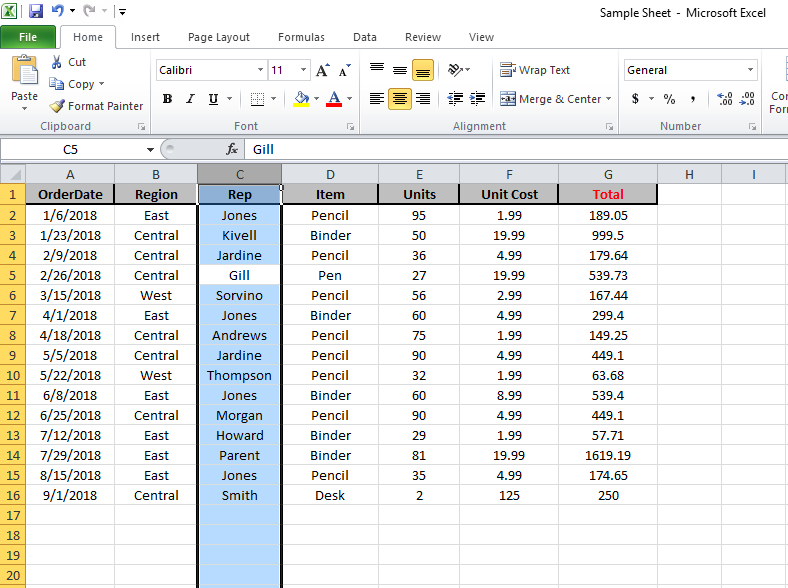
Suppose you have a dataset as shown below and you want to select an entire column (say column C).

The first thing to do is select any cell in Column C.
Once you have any cell in column C selected, use the below keyboard shortcut:
CONTROL + SPACE
Hold the Control key and then press the spacebar key on your keyboard
In case you’re using Excel on Mac, use COMMAND + SPACE
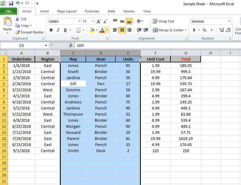
The above shortcut would instantly select the entire column (as you will see it gets highlighted in gray – indicating that it’s selected)

You can use the same shortcut to select multiple contiguous columns as well. For example, suppose you want to select both columns C and D.
To do this, select two adjacent cells (one in column C and one in Column D) and then use the same keyboard shortcut.
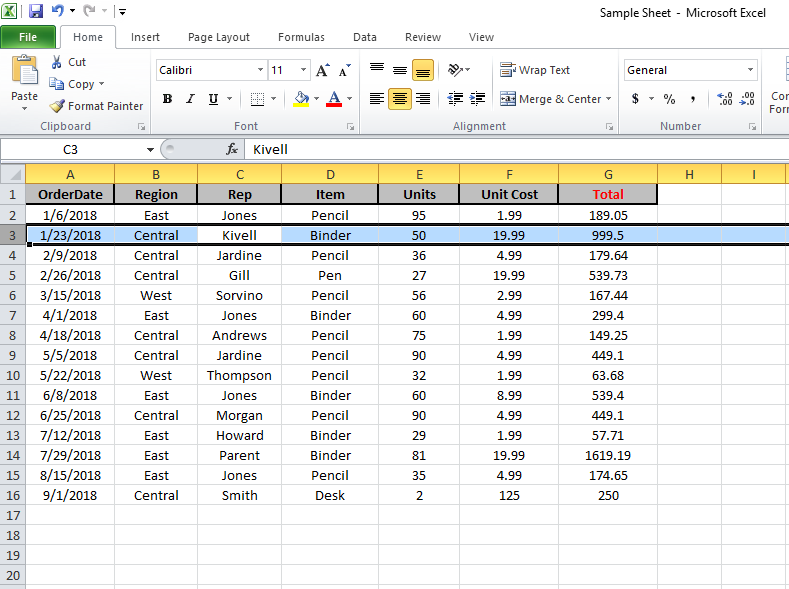
Selecting the Entire Row
If you want to select the entire row, select any cell in the row that you want to be selected and then use the below keyboard shortcut
SHIFT + SPACE
Hold the Shift key and then press the Spacebar key.
You will again see that it gets selected and highlighted in gray.

In case you want to select multiple contiguous rows, select multiple adjacent cells in the same column and then use the keyboard shortcut.
Also read: Select Every Other Row in Excel
Select Entire Column (or Multiple Columns) Using Mouse
I have a feeling you may already know this method, but let me cover it anyway (it will be short).
Select One Column (or Row)
If you want to select an entire column (say column D), hover the cursor over the column headers (where it says D). You will notice that the cursor changes to a black downward-pointing arrow.
Now, click the left mouse key.
Doing this will select the entire column D.

Similarly, if you want to select the entire row, click on the row number (in the row header on the left)
Select Multiple Contiguous Columns (or Rows)
Suppose you want to select multiple columns that are next to each other (say column D, E, and F)
Follow the below steps to do this:
- Place the cursor on the left most column header of column D
- Press the left mouse key and keep it pressed
- With the left key pressed, drag the mouse to also cover column E and F
The above steps would automatically select all the columns in between the first and the last selected column.

And the same way, you can also select multiple contiguous rows.
Select Multiple Non-Contiguous Columns (or Rows)
This is the most common scenario where you need to select multiple columns that are not next to each other (say column D, and F).
Below are the steps to do this:
- Place the cursor at the column heading of one of the columns (say column D in this case)
- Click the mouse left key to select the column
- Press and hold the Control key
- With the Control key pressed, select all the other columns you want to select

You can do the same with rows as well.
Select Entire Column (or Multiple Columns) Using Name Box
Use this method when you want to:
- Select a far-off row or column
- Select multiple contiguous or non-contiguos rows/columns
Name box is a small box that is left of the formula bar.

While the main purpose of the Name Box is to quickly name a cell or range of cells, you can also use it to quickly select any column (or row).
For example, if you want to select the entire column D, enter the following in the name box and hit enter:
D:D
Similarly, if you want to select multiple columns (say D, E, and F), enter the following in the name box:
D:F
And that’s not it!
If you want to select multiple columns that are not adjacent, say D, H, and I, you can enter the below:
D:D,H:H,I:I
When I used to work as a financial analyst years ago, I found this trick extremely useful. It allowed me to quickly select columns and format them at once, or delete/hide these columns in one go.
The Named Range Trick
Let me also show you another wonderful trick.
Suppose you’re working in a workbook where you may often have a need to select far-off columns (say column B, D, and G).
Instead of doing it one by one or entering it manually in the Name Box, here is what you can do – create a named range that refers to the columns you want to select.
Once created, you can simply enter the named range name in the Name box (or select it from the drop-down)
Below are the steps to create a named range for specific columns:
- Select the columns for which you want to create the named range (hold the Control key and then select the columns one-by-one)
- Enter the name you want to give to the selection in the Name Box (no spaces allowed in the name). In this example, I will use the name SalesData

- Hit Enter
Once this is done, you have created a named range in Excel that now refers to the columns you selected (B, D, and G in my example).
And now it’s time for magic.
If you want to quickly select the columns B, D, and G, just enter the name in the Name box and hit enter (or click on the small drop-down icon at the end of the name box and select the name from the list).

Voila, all the columns would be selected.

This technique is useful if you may have a need to select the same columns multiple times in the same sheet.
You can use this technique to select rows as well as different ranges. For example, if you want to select two separate ranges in Excel, just follow the same steps (instead of selected columns, select the ranges and give them a name).
Select Column in an Excel Table
When working with Excel Tables, you may sometimes have a need to select an entire row or column in the table.
This means that you don’t want to select the entire column in the worksheet, but the entire column of the table.
Here is the trick to do this:
- Place the cursor on the header of the Excel table (note this is the header of the column in the Excel table, not the one that displays the column letter)
- You will notice that the cursor would chnage into a downward pointing black arrow

- Click the left mouse key
The above steps would select the entire column in the Excel Table (and not the full column).
And if you want to select multiple columns, hold the Control key and repeat the process for all the columns you want to select.
Also read: AutoSum in Excel (Shortcut)
Select Column in an Pivot Table
Just like the Excel table, you can also quickly select an entire row or column in a Pivot Table.
Suppose you have a Pivot Table as shown below and you want to select the Sales columns,
Below are the steps to do this:
- Place the cursor on the header of the Pivot table header that you want to select
- You will notice that the cursor would chnage into a downward pointing black arrow

- Click the left mouse key
These steps would select the Sales column. Similarly, if you want to select multiple columns, hold the Control key and then make the selection.
So these are some of the common ways you can use to select an entire column or an entire row in Excel.
I hope you found this tutorial useful!
Other Excel tutorials you may also like:
- Flip Data in Excel | Reverse Order of Data in Column/Row
- How to Lock Row Height & Column Width in Excel (Easy Trick)
- How to Delete All Hidden Rows and Columns in Excel
- 7 Easy Ways to Select Multiple Cells in Excel
- How to Insert Multiple Rows in Excel
- How to Copy and Paste Column in Excel? 3 Easy Ways!
- How to Multiply a Column by a Number in Excel
- Select Till End of Data in a Column in Excel (Shortcuts)
- How to Group Columns in Excel?
Select cell contents in Excel
In Excel, you can select cell contents of one or more cells, rows and columns.
Note: If a worksheet has been protected, you might not be able to select cells or their contents on a worksheet.
Select one or more cells
-
Click on a cell to select it. Or use the keyboard to navigate to it and select it.
-
To select a range, select a cell, then with the left mouse button pressed, drag over the other cells.
Or use the Shift + arrow keys to select the range.
-
To select non-adjacent cells and cell ranges, hold Ctrl and select the cells.
Select one or more rows and columns
-
Select the letter at the top to select the entire column. Or click on any cell in the column and then press Ctrl + Space.
-
Select the row number to select the entire row. Or click on any cell in the row and then press Shift + Space.
-
To select non-adjacent rows or columns, hold Ctrl and select the row or column numbers.
Select table, list or worksheet
-
To select a list or table, select a cell in the list or table and press Ctrl + A.
-
To select the entire worksheet, click the Select All button at the top left corner.
Note: In some cases, selecting a cell may result in the selection of multiple adjacent cells as well. For tips on how to resolve this issue, see this post How do I stop Excel from highlighting two cells at once? in the community.
|
To select |
Do this |
|---|---|
|
A single cell |
Click the cell, or press the arrow keys to move to the cell. |
|
A range of cells |
Click the first cell in the range, and then drag to the last cell, or hold down SHIFT while you press the arrow keys to extend the selection. You can also select the first cell in the range, and then press F8 to extend the selection by using the arrow keys. To stop extending the selection, press F8 again. |
|
A large range of cells |
Click the first cell in the range, and then hold down SHIFT while you click the last cell in the range. You can scroll to make the last cell visible. |
|
All cells on a worksheet |
Click the Select All button.
To select the entire worksheet, you can also press CTRL+A. Note: If the worksheet contains data, CTRL+A selects the current region. Pressing CTRL+A a second time selects the entire worksheet. |
|
Nonadjacent cells or cell ranges |
Select the first cell or range of cells, and then hold down CTRL while you select the other cells or ranges. You can also select the first cell or range of cells, and then press SHIFT+F8 to add another nonadjacent cell or range to the selection. To stop adding cells or ranges to the selection, press SHIFT+F8 again. Note: You cannot cancel the selection of a cell or range of cells in a nonadjacent selection without canceling the entire selection. |
|
An entire row or column |
Click the row or column heading.
1. Row heading 2. Column heading You can also select cells in a row or column by selecting the first cell and then pressing CTRL+SHIFT+ARROW key (RIGHT ARROW or LEFT ARROW for rows, UP ARROW or DOWN ARROW for columns). Note: If the row or column contains data, CTRL+SHIFT+ARROW key selects the row or column to the last used cell. Pressing CTRL+SHIFT+ARROW key a second time selects the entire row or column. |
|
Adjacent rows or columns |
Drag across the row or column headings. Or select the first row or column; then hold down SHIFT while you select the last row or column. |
|
Nonadjacent rows or columns |
Click the column or row heading of the first row or column in your selection; then hold down CTRL while you click the column or row headings of other rows or columns that you want to add to the selection. |
|
The first or last cell in a row or column |
Select a cell in the row or column, and then press CTRL+ARROW key (RIGHT ARROW or LEFT ARROW for rows, UP ARROW or DOWN ARROW for columns). |
|
The first or last cell on a worksheet or in a Microsoft Office Excel table |
Press CTRL+HOME to select the first cell on the worksheet or in an Excel list. Press CTRL+END to select the last cell on the worksheet or in an Excel list that contains data or formatting. |
|
Cells to the last used cell on the worksheet (lower-right corner) |
Select the first cell, and then press CTRL+SHIFT+END to extend the selection of cells to the last used cell on the worksheet (lower-right corner). |
|
Cells to the beginning of the worksheet |
Select the first cell, and then press CTRL+SHIFT+HOME to extend the selection of cells to the beginning of the worksheet. |
|
More or fewer cells than the active selection |
Hold down SHIFT while you click the last cell that you want to include in the new selection. The rectangular range between the active cell and the cell that you click becomes the new selection. |
Need more help?
You can always ask an expert in the Excel Tech Community or get support in the Answers community.
See Also
Select specific cells or ranges
Add or remove table rows and columns in an Excel table
Move or copy rows and columns
Transpose (rotate) data from rows to columns or vice versa
Freeze panes to lock rows and columns
Lock or unlock specific areas of a protected worksheet
Need more help?
Author: Oscar Cronquist Article last updated on March 06, 2023
I will in this article demonstrate several techniques that extract or filter records based on two conditions applied to a single column in your dataset. For example, if you use the array formula then the result will refresh instantly when you enter new start and end values.
The remaining built-in techniques need a little more manual work in order to apply new conditions, however, they are fast. The downside with the array formula is that it may become slow if you are working with huge amounts of data.
I have also written an article in case you need to find records that match one condition in one column and another condition in another column. The following article shows you how to build a formula that uses an arbitrary number of conditions: Extract records where all criteria match if not empty
This article Extract records between two dates is very similar to the current one you are reading right now, Excel dates are actually numbers formatted as dates in Excel. If you want to search for a text string within a given date range then read this article: Filter records based on a date range and a text string
I must recommend this article if you want to do a wildcard search across all columns in a data set, it also returns all matching records. If you want to extract records based on criteria and not a numerical range then read this part of this article.
What is on this page?
- Extract all rows from a range based on range criteria (Array formula)
- Video
- How to enter an array formula
- Explaining array formula
- Extract all rows from a range based on range criteria — Excel 365
- Explaining formula
- Extract all rows from a range based on multiple conditions (Array formula)
- Explaining array formula
- Extract all rows from a range based on multiple conditions — Excel 365
- Explaining formula
- Extract all rows from a range based on range critera
[Excel defined Table] - Extract all rows from a range based on range critera
[AutoFilter] - Extract all rows from a range based on range criteria
[Advanced Filter] - Get Excel file
1. Extract all rows from a range based on range criteria
[Array formula]
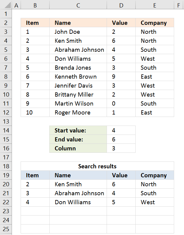
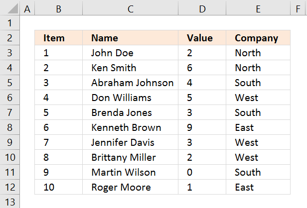
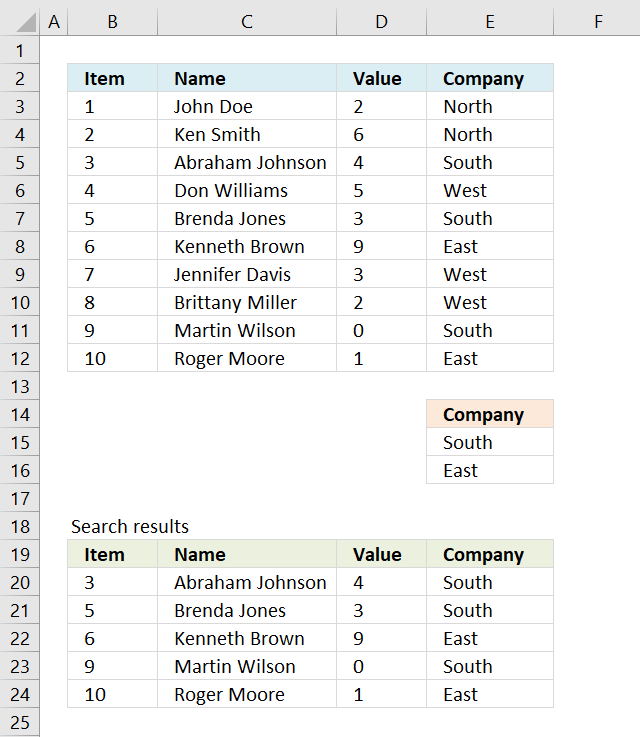
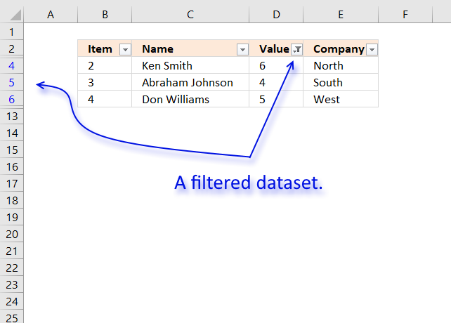
The picture above shows you a dataset in cell range B3:E12, the search parameters are in D14:D16. The search results are in B20:E22.
Cells D14 allows you to specify the start number, and cell D15 is the end number of the range. Cell D16 determines which column to use in cell range B3:E12.
The result is presented in cells B20:E20 and cells below. The example above shows a start value of 4 and an end value of 6, the column is three meaning the third column in cell range B3:E12.
All records that match range 4 to 6 in cell range D3:D12 are extracted, D3:D12 is the third column in B3:E12.
Update 20 Sep 2017, a smaller formula in cell A20.
Array formula in cell A20:
=INDEX($B$3:$E$12, SMALL(IF((INDEX($B$3:$E$12, , $D$16)< =$D$15)*(INDEX($B$3:$E$12, , $D$16)> =$D$14), MATCH(ROW($B$3:$E$12), ROW($B$3:$E$12)), «»), ROWS(B20:$B$20)), COLUMNS($A$1:A1))
Back to top
1.1 Video
See this video to learn more about the formula:
Back to top
1.2 How to enter this array formula
- Select cell A20
- Paste above formula to cell or formula bar
- Press and hold CTRL + SHIFT simultaneously
- Press Enter once
- Release all keys
The formula bar now shows the formula with a beginning and ending curly bracket, that is if you did the above steps correctly. Like this:
{=array_formula}
Don’t enter these characters yourself, they appear automatically.
Now copy cell A20 and paste to cell range A20:E22.
Back to top
1.3 Explaining array formula in cell A20
You can follow along if you select cell A19, go to tab «Formulas» on the ribbon and press with left mouse button on the «Evaluate Formula» button.
Step 1 — Filter a specific column in cell range B3:E12
The INDEX function is mostly used for getting a single value from a given cell range, however, it can also return an entire column or row from a cell range.
This is exactly what I am doing here, the column number specified in cell D16 determines which column to extract.
INDEX($B$3:$E$12, , $D$16, 1)
becomes
INDEX($B$3:$E$12, , 3, 1)
and returns C3:C12.
Recommended articles
Step 2 — Check which values are smaller or equal to the condition
The smaller than and equal sign are logical operators that let you compare value to value, in this case, if a number is smaller than or equal to another number.
The output is a boolean value, True och False. Their positions in the array correspond to the positions in the cell range.
INDEX($B$3:$E$12, , $D$16, 1)< =$D$15
becomes
C3:C12< =$D$15
becomes
{2; 6; 4; 5; 3; 9; 3; 2; 0; 1}<=6
and returns
{TRUE; TRUE; TRUE; TRUE; TRUE; FALSE; TRUE; TRUE; TRUE; TRUE}.
Step 3 — Multiply arrays — AND logic
There is a second condition we need to evaluate before we know which records are in range.
(INDEX($B$3:$E$12, , $D$16, 1)< =$D$15)*(INDEX($B$3:$E$12, , $D$16, 1)> =$D$14)
becomes
({2; 6; 4; 5; 3; 9; 3; 2; 0; 1}< =$C$14)*({2; 6; 4; 5; 3; 9; 3; 2; 0; 1}> =$C$13)
becomes
({2; 6; 4; 5; 3; 9; 3; 2; 0; 1}< =3)*({2; 6; 4; 5; 3; 9; 3; 2; 0; 1}> =0)
becomes
{TRUE; FALSE; FALSE; FALSE; TRUE; FALSE; TRUE; TRUE; TRUE; TRUE}*{TRUE; TRUE; TRUE; TRUE; TRUE; TRUE; TRUE; TRUE; TRUE; TRUE}
Both conditions must be met, the asterisk lets us multiple the arrays meaning AND logic.
TRUE * TRUE equals FALSE, all other combinations return False. TRUE * FALSE equals FALSE and so on.
{TRUE; FALSE; FALSE; FALSE; TRUE; FALSE; TRUE; TRUE; TRUE; TRUE} * {TRUE; TRUE; TRUE; TRUE; TRUE; TRUE; TRUE; TRUE; TRUE; TRUE}
returns
{1; 0; 0; 0; 1; 0; 1; 1; 1; 1}.
Boolean values have numerical equivalents, TRUE = 1 and FALSE equals 0 (zero). They are converted when you perform an arithmetic operation in a formula.
Step 4 — Create number sequence
The ROW function calculates the row number of a cell reference.
ROW(reference)
ROW($B$3:$E$12)
returns
{3; 4; 5; 6; 7; 8; 9; 10; 11; 12}.
Step 5 — Create a number sequence from 1 to n
The MATCH function returns the relative position of an item in an array or cell reference that matches a specified value in a specific order.
MATCH(ROW($B$3:$E$12), ROW($B$3:$E$12))
becomes
MATCH({3; 4; 5; 6; 7; 8; 9; 10; 11; 12}, {3; 4; 5; 6; 7; 8; 9; 10; 11; 12})
and returns
{1; 2; 3; 4; 5; 6; 7; 8; 9; 10}.
Step 6 — Return the corresponding row number
The IF function returns one value if the logical test is TRUE and another value if the logical test is FALSE.
IF(logical_test, [value_if_true], [value_if_false])
IF((INDEX($B$3:$E$12, , $D$16)< =$D$15)*(INDEX($B$3:$E$12, , $D$16)> =$D$14), MATCH(ROW($B$3:$E$12), ROW($B$3:$E$12)), «»)
becomes
IF({1; 0; 0; 0; 1; 0; 1; 1; 1; 1}, MATCH(ROW($B$3:$E$12), ROW($B$3:$E$12)), «»)
becomes
IF({1; 0; 0; 0; 1; 0; 1; 1; 1; 1}, {1; 2; 3; 4; 5; 6; 7; 8; 9; 10}, «»)
and returns
{1; «»; «»; «»; 5; «»; 7; 8; 9; 10}.
Step 7 — Extract k-th smallest row number
The SMALL function returns the k-th smallest value from a group of numbers.
SMALL(array, k)
SMALL(IF((INDEX($B$3:$E$12, , $D$16)< =$D$15)*(INDEX($B$3:$E$12, , $D$16)> =$D$14), MATCH(ROW($B$3:$E$12), ROW($B$3:$E$12)), «»), ROWS(B20:$B$20))
becomes
SMALL({1; «»; «»; «»; 5; «»; 7; 8; 9; 10}, ROWS(B20:$B$20))
becomes
SMALL({1; «»; «»; «»; 5; «»; 7; 8; 9; 10}, 1)
and returns 1.
Step 8 — Return the entire row record from the cell range
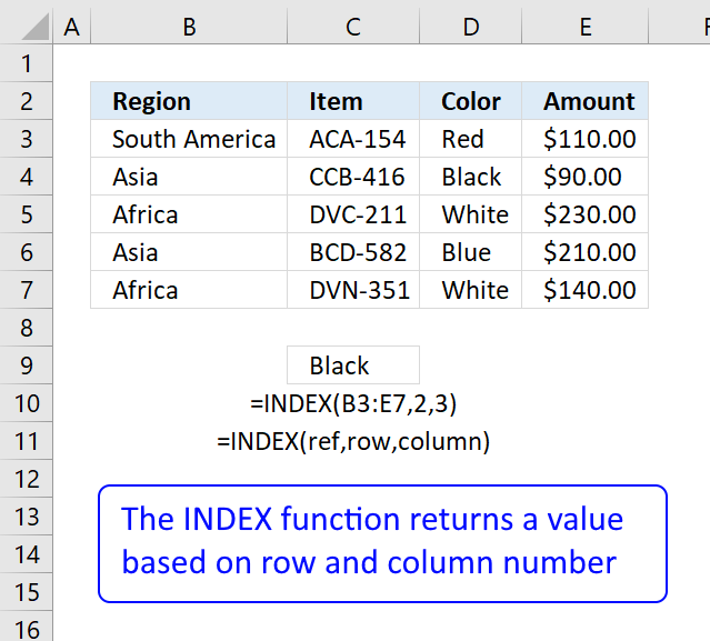
The INDEX function returns a value from a cell range, you specify which value based on a row and column number.
INDEX(array, [row_num], [column_num])
INDEX($B$3:$E$12, SMALL(IF((INDEX($B$3:$E$12, , $D$16)< =$D$15)*(INDEX($B$3:$E$12, , $D$16)> =$D$14), MATCH(ROW($B$3:$E$12), ROW($B$3:$E$12)), «»), ROWS(B20:$B$20)), COLUMNS($A$1:A1))
becomes
INDEX($B$3:$E$12, 1, , 1)
and returns {2, «Ken Smith», 6, «North»}.
Back to top
Recommended articles
Back to top
2. Extract all rows from a range based on range criteria — Excel 365
Update 17 December 2020, the new FILTER function is now available for Excel 365 users.
Excel 365 dynamic array formula in cell B20:
=FILTER($B$3:$E$12, (D3:D12<=D15)*(D3:D12>=D14))
It is a regular formula, however, it returns an array of values and extends automatically to cells below and to the right. Microsoft calls this a dynamic array and spilled array.
The array formula below is for earlier Excel versions, it searches for values that meet a range criterion (cell D14 and D15), the formula lets you change the column to search in with cell D16.
This formula can be used with whatever dataset size and shape. To search the first column, type 1 in cell D16. This is a great improvement in both formula size and how easy it is to enter the formula, compared to the array formula in section 1.
Back to top
2.1 Explaining array formula
Step 1 — First condition
The less than character and the equal sign are both logical operators meaning they are able to compare value to value, the output is a boolean value.
In this case, the logical expression evaluates if numbers in D3:D12 are smaller than or equal to the condition specified in cell D15.
D3:D12<=D15
becomes
{2;6;4;5;3;9;3;2;0;1}<=6
and returns
{TRUE; TRUE; TRUE; TRUE; TRUE; FALSE; TRUE; TRUE; TRUE; TRUE}.
Step 2 — Second condition
The second condition checks if the number in D3:D12 are larger than or equal to the condition specified in cell D14.
D3:D12>=D14
becomes
{2;6;4;5;3;9;3;2;0;1}>=4
and returns
{FALSE; TRUE; TRUE; TRUE; FALSE; TRUE; FALSE; FALSE; FALSE; FALSE}.
Step 3 — Multiply arrays — AND logic
The asterisk lets you multiply a number to a number, in this case, array to array. Both arrays must be of the exact same size.
The parentheses let you control the order of operation, we want to evaluate the comparisons first before we multiply the arrays.
(D3:D12<=D15)*(D3:D12>=D14)
becomes
{TRUE; TRUE; TRUE; TRUE; TRUE; FALSE; TRUE; TRUE; TRUE; TRUE}*{FALSE; TRUE; TRUE; TRUE; FALSE; TRUE; FALSE; FALSE; FALSE; FALSE}
and returns
{0; 1; 1; 1; 0; 0; 0; 0; 0; 0}.
AND logic works like this:
TRUE * TRUE = TRUE (1)
TRUE * FALSE = FALSE (0)
FALSE * TRUE = FALSE (0)
FALSE * FALSE = FALSE (0)
Note that multiplying boolean values returns their numerical equivalents.
TRUE = 1 and FALSE = 0 (zero).
Step 4 — Filter values based on the array
The FILTER function lets you extract values/rows based on a condition or criteria.
FILTER(array, include, [if_empty])
FILTER($B$3:$E$12, (D3:D12<=D15)*(D3:D12>=D14))
becomes
FILTER({1, «John Doe», 2, «North»; 2, «Ken Smith», 6, «North»; 3, «Abraham Johnson», 4, «South»; 4, «Don Williams», 5, «West»; 5, «Brenda Jones», 3, «South»; 6, «Kenneth Brown», 9, «East»; 7, «Jennifer Davis», 3, «West»; 8, «Brittany Miller», 2, «West»; 9, «Martin Wilson», 0, «South»; 10, «Roger Moore», 1, «East»}, (D3:D12<=D15)*(D3:D12>=D14))
becomes
FILTER({1, «John Doe», 2, «North»; 2, «Ken Smith», 6, «North»; 3, «Abraham Johnson», 4, «South»; 4, «Don Williams», 5, «West»; 5, «Brenda Jones», 3, «South»; 6, «Kenneth Brown», 9, «East»; 7, «Jennifer Davis», 3, «West»; 8, «Brittany Miller», 2, «West»; 9, «Martin Wilson», 0, «South»; 10, «Roger Moore», 1, «East»}, {0; 1; 1; 1; 0; 0; 0; 0; 0; 0})
and returns
{2, «Ken Smith», 6, «North»; 3, «Abraham Johnson», 4, «South»; 4, «Don Williams», 5, «West»}.
Back to top
3. Extract all rows from a range that meet the criteria in one column [Array formula]
The array formula in cell B20 extracts records where column E equals either «South» or «East». You can use as many conditions as you like as long as you adjust the cell reference $E$15:$E$16 accordingly in the formula below.
The following array formula in cell B20 is for earlier Excel versions than Excel 365:
=INDEX($B$3:$E$12, SMALL(IF(COUNTIF($E$15:$E$16,$E$3:$E$12), MATCH(ROW($B$3:$E$12), ROW($B$3:$E$12)), «»), ROWS(B20:$B$20)), COLUMNS($B$2:B2))
To enter an array formula, type the formula in a cell then press and hold CTRL + SHIFT simultaneously, now press Enter once. Release all keys.
The formula bar now shows the formula with a beginning and ending curly bracket telling you that you entered the formula successfully. Don’t enter the curly brackets yourself.
Back to top
3.1 Explaining formula in cell B20
Step 1 — Filter a specific column in cell range $A$2:$D$11
The COUNTIF function allows you to identify cells in range $E$3:$E$12 that equals $E$15:$E$16.
COUNTIF($E$15:$E$16,$E$3:$E$12)
becomes
COUNTIF({«South»; «East»},{«North»; «North»; «South»; «West»; «South»; «East»; «West»; «West»; «South»; «East»})
and returns
{0;0;1;0;1;1;0;0;1;1}.
Step 2 — Return corresponding row number
The IF function has three arguments, the first one must be a logical expression. If the expression evaluates to TRUE then one thing happens (argument 2) and if FALSE another thing happens (argument 3).
The logical expression was calculated in step 1 , TRUE equals 1 and FALSE equals 0 (zero).
IF(COUNTIF($E$15:$E$16,$E$3:$E$12), MATCH(ROW($B$3:$E$12), ROW($B$3:$E$12)), «»)
becomes
IF({0; 0; 1; 0; 1; 1; 0; 0; 1; 1}, MATCH(ROW($B$3:$E$12), ROW($B$3:$E$12)), «»)
becomes
IF({0; 0; 1; 0; 1; 1; 0; 0; 1; 1}, {1; 2; 3; 4; 5; 6; 7; 8; 9; 10}, «»)
and returns
{«»; «»; 3; «»; 5; 6; «»; «»; 9; 10}.
Step 3 — Find k-th smallest row number
SMALL(IF(COUNTIF($E$15:$E$16,$E$3:$E$12), MATCH(ROW($B$3:$E$12), ROW($B$3:$E$12)), «»), ROWS(B20:$B$20))
becomes
SMALL({«»; «»; 3; «»; 5; 6; «»; «»; 9; 10}, ROWS(B20:$B$20))
becomes
SMALL({«»; «»; 3; «»; 5; 6; «»; «»; 9; 10}, 1)
and returns 3.
Step 4 — Return value based on row and column number
The INDEX function returns a value based on a cell reference and column/row numbers.
INDEX($B$3:$E$12, SMALL(IF(COUNTIF($E$15:$E$16,$E$3:$E$12), MATCH(ROW($B$3:$E$12), ROW($B$3:$E$12)), «»), ROWS(B20:$B$20)), COLUMNS($B$2:B2))
becomes
INDEX($B$3:$E$12, 3, COLUMNS($B$2:B2))
becomes
INDEX($B$3:$E$12, 3, 1)
and returns 3 in cell B20.
Back to top
Recommended articles
Back to top
4. Extract all rows from a range based on multiple conditions — Excel 365
Update 17 December 2020, the new FILTER function is now available for Excel 365 users.
Excel 365 dynamic array formula in cell B20:
=FILTER($B$3:$E$12, COUNTIF(E15:E16, E3:E12))
It is a regular formula, however, it returns an array of values. Read here how it works: Filter values based on criteria
The formula extends automatically to cells below and to the right. Microsoft calls this a dynamic array and spilled array.
Back to top
4.1 Explaining array formula
Step 1 — Check if values equal criteria
The COUNTIF function calculates the number of cells that meet a given condition.
COUNTIF(range, criteria)
COUNTIF($E$15:$E$16,$E$3:$E$12)
becomes
COUNTIF({«South»; «East»},{«North»; «North»; «South»; «West»; «South»; «East»; «West»; «West»; «South»; «East»})
and returns
{0; 0; 1; 0; 1; 1; 0; 0; 1; 1}.
Step 2 — Filter records based on array
The FILTER function lets you extract values/rows based on a condition or criteria.
FILTER(array, include, [if_empty])
FILTER($B$3:$E$12, COUNTIF(E15:E16, E3:E12))
becomes
FILTER($B$3:$E$12, {0; 0; 1; 0; 1; 1; 0; 0; 1; 1})
and returns
{3, «Abraham Johnson», 4, «South»; 5, «Brenda Jones», 3, «South»; 6, «Kenneth Brown», 9, «East»; 9, «Martin Wilson», 0, «South»; 10, «Roger Moore», 1, «East»}.
Back to top
5. Extract all rows from a range that meet the criteria in one column [Excel defined Table]
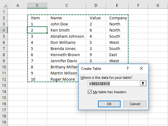
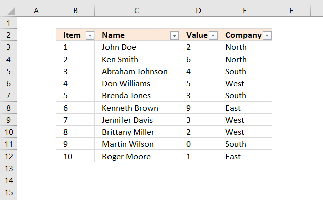
The image above shows a dataset converted to an Excel defined Table, a number filter has been applied to the third column in the table.
Here are the instructions to create an Excel Table and filter values in column 3.
- Select a cell in the dataset.
- Press CTRL + T

- Press with left mouse button on check box «My table has headers».
- Press with left mouse button on OK button.

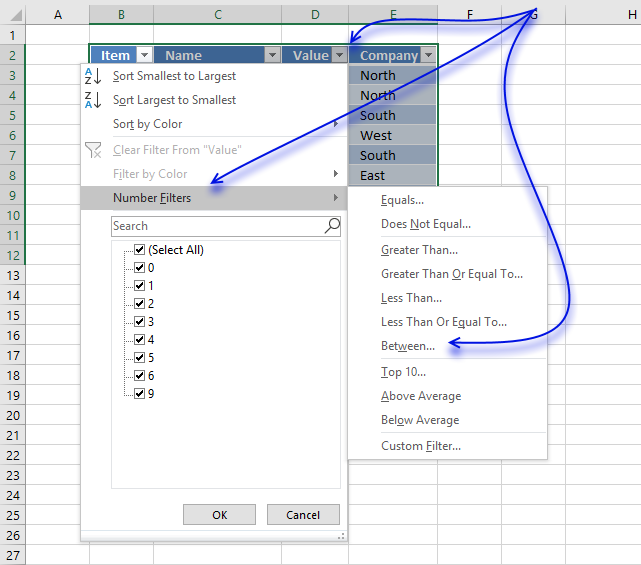
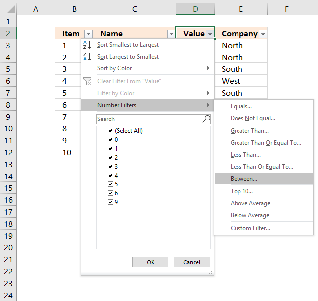
The image above shows the Excel defined Table, here is how to filter D between 4 and 6:
- Press with left mouse button on black arrow next to header.
- Press with left mouse button on «Number Filters».
- Press with left mouse button on «Between…».

- Type 4 and 6.

- Press with left mouse button on OK button.

Back to top
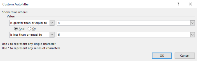
6. Extract all rows from a range that meet the criteria in one column [AutoFilter]
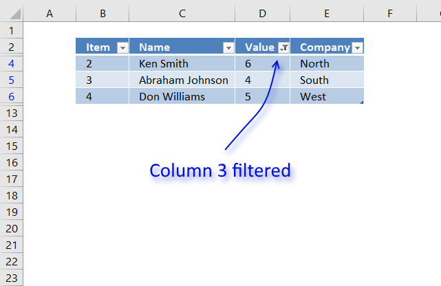
The image above shows filtered records based on two conditions, values in column D are larger or equal to 4 or smaller or equal to 6.
Here is how to apply Filter arrows to a dataset.
- Select any cell within the dataset range.
- Go to tab «Data» on the ribbon.
- Press with left mouse button on «Filter button».

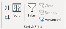
Black arrows appear next to each header.
Lets filter records based on conditions applied to column D.
- Press with left mouse button on the black arrow next to the header in Column D, see the image below.
- Press with left mouse button on «Number Filters».
- Press with left mouse button on «Between».

- Type 4 and 6 in the dialog box shown below.
- Press with left mouse button on OK button.
Back to top
7. Extract all rows from a range that meet the criteria in one column
[Advanced Filter]
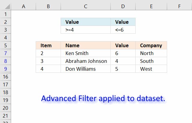
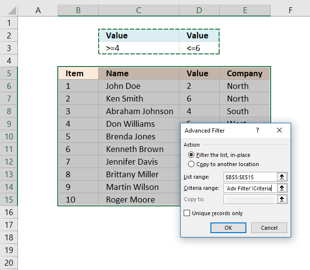
The image above shows a filtered dataset in cell range B5:E15 using Advanced Filter which is a powerful feature in Excel.
Here is how to apply a filter:
- Create headers for the column you want to filter, preferably above or below your data set.
Your filters will possibly disappear if placed next to the data set because rows may become hidden when the filter is applied. - Select the entire dataset including headers.
- Go to tab «Data» on the ribbon.
- Press with left mouse button on the «Advanced» button.

- A dialog box appears.

- Select the criteria range C2:D3, shown ithe n above image.
- Press with left mouse button on OK button.
Back to top
Recommended articles
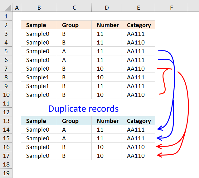
Extract duplicate records
This article describes how to filter duplicate rows with the use of a formula. It is, in fact, an array […]
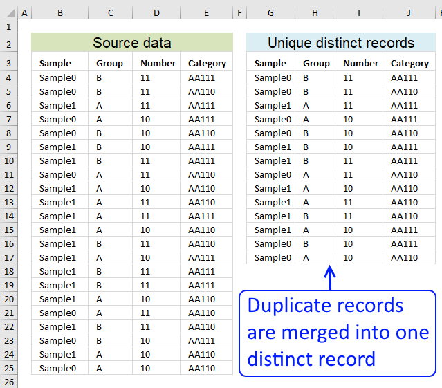
Filter unique distinct records
Table of contents Filter unique distinct row records Filter unique distinct row records but not blanks Filter unique distinct row […]
Back to top
8. Excel file
Back to top
In this article, we will learn how to select an entire column in excel and how to select whole row or a table using keyboard shortcut keys. While preparing reports and dashboard in Excel, it’s time-consuming to select an entire column using the mouse. These excel shortcuts are useful to save time and help you do your work faster using the keyboard shortcut keys. How to select row with the Excel shortcut?
Selecting cells is a very common function in Excel. It performs many tasks like addition, deletion and width adjustment of multiple rows and columns while applying the formula on data in Excel. Shortcut keys to select all rows and columns can provide an easier and quicker method of using MS Excel 2016. We have a data set here, let’s understand with the example.
How to Select Column in Excel Using Keyboard Shortcuts (CTRL+SPACE)
While navigating on an excel sheet with large data, excel column selection is very basic yet important task. Let’s see how easy is selecting columns in excel.
- Select any cell in any column.
- Press Ctrl + Space shortcut keys on the keyboard. The whole column will be highlighted in excel to show the selected column, as shown below in the picture. You can also say that this is a shortcut to highlight column in excel.
If you wish to select the adjacent columns with the selected column, use Shift + Left/Right arrow key(s) to select entire columns left or right of that column. You can go either way but can’t select both sides of column.
Let’s Select Entire Columns C to E
- To Select Column C:E, Select any cell of the 3rd column.
- Use Ctrl + Space shortcut keys from your keyboard to select column E (Leave the keys if the column is selected).
- Now use Shift + Right (twice) arrow keys to select columns D and E, simultaneously.
- You can select columns C:A by using shortcut Shift + Left (twice) arrow keys.
- You can select columns to the end of sheet using Ctrl+Shift + Left shortcut.
- To select to end of column from a cell, use excel shortcut Ctrl+Shift + Down arrow.
You can’t select columns A:E if you start from any column in between. I am repeating, you can only select entire columns in Excel from left or right of initial column.
How to Select Entire Row Using Keyboard Shortcuts in Excel (SHIFT+SPACE)
This command is used for selecting rows in excel. This is also a shortcut to highlight a row in excel.
- Select the cell in the row you wish to select.
- Press Shift+ Space key to select the row on the selected cell (release the keys, if the row is selected).
- If you wish to select the adjacent rows with the selected row, press Shift+ Up/down arrow key(s) to select the UP or DOWN to that row. You can go either way but can’t access both sides of it.
Selecting 3rd to 5th whole rows of the sheet can be done in two ways:
- Select any cell of the 3rd row, press Shift + Space key to select the row.
- Now use Shift + Down(twice) arrow key to select the 4th and the 5th row.
- Or you could go another way from 5th to 3rd row but you won’t be able to select 3rd and 5th row both, starting from the 4th row.

Select multiple rows and columns of a table with shortcut keys and perform your tasks efficiently.
Frequently Asked Question:
How to apply formula to entire column?
Easy, write a formula in the first cell of column and press CTRL + SPACE to select entire column and then CTRL+D to apply formula to entire column.
How to select all in excel?
To select all data press CTRL+A.
How to highlight a row in excel?
Just select any cell in the row you want to highlight and Press Shift+ Space.
How to select multiple cells in Excel mac?
Hold down the command key and scroll over the cells to select. If the cells are not adjacent then click on the cells while holding the command key.
Hope you understood how to select columns and rows with shortcuts in Excel. You can perform these tasks in 2013 and 2010. Explore more links on shortcut keys here. If you have any query, please mention in the comment box below. We will help you.
If you liked our blogs, share it with your friends on Facebook. And also you can follow us on Twitter and Facebook.
We would love to hear from you, do let us know how we can improve, complement or innovate our work and make it better for you. Write us at info@exceltip.com