
Содержание
- How to Find Blank / Empty Cells in Excel & Google Sheets
- Find & Select Empty Cells
- Find Blank Cells in Google Sheets
- How to find blank cells in Excel using the Go To feature
- How to Find Blank Cells in Excel using Go To
- How to select and highlight blank cells in Excel
- Select and highlight empty cells with Go To Special
- Filter and highlight blanks in a specific column
- How to highlight blank cells in Excel with conditional formatting
- Example 1. Highlight all blank cells in a range
- Example 2. Highlight rows that have blanks in a specific column
- Highlight if blank with VBA
- Macro 1: Color blank cells
- Macro 2: Color blanks and empty strings
- How to insert and run macro
- Excel VBA, find the next empty cell
- 2 Answers 2
- How to fill empty cells with 0, with value above/below in Excel
- How to select empty cells in Excel worksheets
- Excel formula to fill in blank cells with value above / below
- Use the Fill Blank Cells add-in by Ablebits
- Fill empty cells with 0 or another specific value
- Method 1
- Method 2
How to Find Blank / Empty Cells in Excel & Google Sheets
In this tutorial, you will learn how to find blank cells in Excel and Google Sheets.
![]()
Find & Select Empty Cells
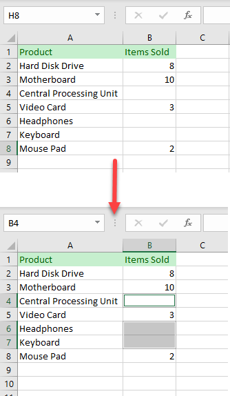
There is an easy way to select all the blank cells in any selected range in Excel. Although this method won’t show you the number of blank cells, it will highlight all of them so you can easily locate them in a spreadsheet.
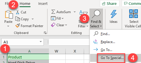
1. First, select the entire data range. Then in the Ribbon, go to Home > Find & Select > Go To Special.
![]()
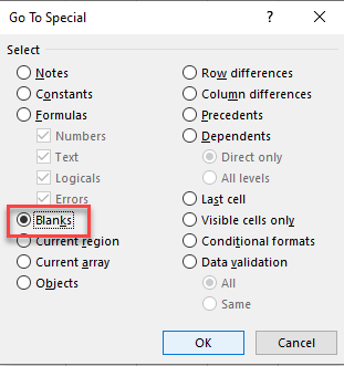
2. In Go To Special dialog window click on Blanks and when done press OK.
![]()
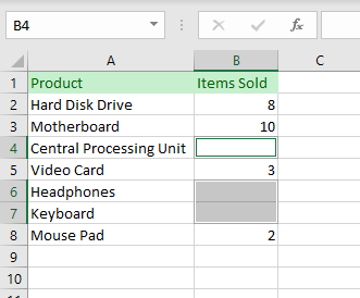
As a result, all blank cells are selected.
![]()
With this method, you won’t find pseudo-blank cells (cells with formulas that return blanks and cells containing only spaces).
Other ways to identify blanks:
Find Blank Cells in Google Sheets
Unlike Excel, Google Sheets doesn’t have a Go To Special feature. But you can identify blank cells and select them one-by-one, highlight them, or replace them.
Источник
How to find blank cells in Excel using the Go To feature
![]()
In Excel, a blank cell doesn’t always mean a cell with an empty string («»). An example to this is invisible characters like a new line character which can be entered by pressing the Alt + Enter key combination when you’re in a cell. You can detect the cells that are actually blank by using Excel’s Go To feature. In this article, we’re going to show you how to find blank cells in Excel using the Go To feature.
![]()
How to Find Blank Cells in Excel using Go To
- Begin by selecting your data including the blank rows
- Open the Go To Special dialog by following HOME > Find & Select > Go To Special in the ribbon
- Select the Blanks option
- Click OK to apply your selection
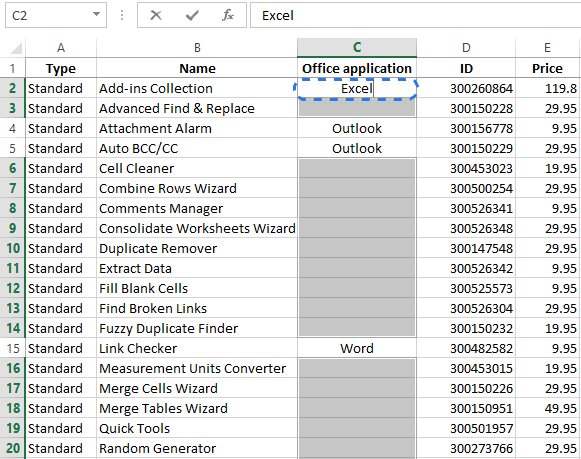
In our example, you can see that Excel selects only two cells, D6 and C7, even though the cells F6 and F7 look empty as well. This is not an error, but an example of «actually not blank cells». The cells like F6 and F7 will also affect results of the COUNTA function, which also counts these types of cells. For example, the =COUNTA(B3:F8) formula returns 28 as it ignores only cells D6 and C7.
You might want to be extra careful when removing blank rows using the Go To feature, because it selects individual blank cells in rows that have values. Removing them will cause data loss, even though you can revert your actions with Undo.
Источник
How to select and highlight blank cells in Excel
 by Svetlana Cheusheva, updated on March 14, 2023
The article shows how to find and highlight blanks in Excel with the help of conditional formatting and VBA. Depending on your needs, you can color only truly blank cells or those that contain zero-length strings as well.
When you receive an Excel file from someone or import it from an external database, it’s always a good idea to check the data to make sure there are no gaps or missing data points. In a small dataset, you can easily spot all the blanks with your own eyes. But if you have a huge file containing hundreds or even thousands of rows, pinpointing empty cells manually is next to impossible.
This tutorial will teach you 4 quick and easy ways to highlight blank cells in Excel so that you can visually identify them. Which method is the best? Well, that depends on the data structure, your goals and your definition of «blanks».
Select and highlight empty cells with Go To Special
This simple method selects all blank cells in a given range, which you can then fill with any color of your choosing.
To select blank cells in Excel, this is what you need to do:
- Select the range where you want to highlight blank. To select all cells with data, click the upper-left cell and press Ctrl + Shift + End to extend the selection to the last used cell.
- On the Home tab, in the Editing group, click Find & Select >Go to Special. Or press F5 and click Special… .

- In the Go To Special dialog box, select Blanks and click OK. This will select all empty cells in the range.
- With the blank cells selected, click the Fill Color icon on the Home tab, in the Font group, and pick the desired color. Done!

- The Go To Special feature only selects truly blank cells, i.e. cells that contain absolutely nothing. Cells containing empty string, spaces, carriage returns, non-printing characters, etc. are not considered blank and are not selected. To highlight cells with formulas that return an empty string («») as the result, use either Conditional Formatting or VBA macro.
- This method is static and is best to be used as a one-time solution. Changes that you make later won’t be reflected automatically: new blanks won’t be highlighted and former blanks that you fill with values will stay colored. If you are looking for a dynamic solution, you’d better use the Conditional Formatting approach.
Filter and highlight blanks in a specific column
If you do not care about empty cells anywhere in the table but rather want to find and highlight cells or the entire rows that have blanks in a certain column, Excel Filter can be the right solution.
To have it done, carry out these steps:
- Select any cell within your dataset and click Sort & Filter >Filter on the Home tab. Or press the CTRL + Shift + L shortcut to turn on auto-filters.
- Click the drop-down arrow for the target column and filter blank values. For this, clear the Select All box, and then select (Blanks).
- Select the filtered cells in the key column or entire rows and choose the Fill color that you want to apply.
In our sample table, this is how we can filter, and then highlight the rows where the SKU cells are empty:
![]()
- Unlike the previous method, this approach regards formulas that return empty strings («») as blank cells.
- This solution is not suitable for frequently changed data because you would have to clean up and highlight again with each change.
How to highlight blank cells in Excel with conditional formatting
Both techniques discussed earlier are straightforward and concise, but they do have a significant drawback — neither method reacts to changes made to the dataset. Unlike them, Conditional Formatting is a dynamic solution, meaning you need to set up the rule just once. As soon as an empty cell is populated with any value, the color will immediately go away. And conversely, once a new blank appears, it will get highlighted automatically.
Example 1. Highlight all blank cells in a range
To highlight all empty cells in a given range, configure the Excel conditional formatting rule in this way:
- Select the range in which you want to highlight blank cells (A2:E6 in our case).
- On the Home tab, in the Styles group, click New Rule >Use a formula to determine which cells to format.
- In the Format values where this formula is true box, enter one of the below formulas, where A2 is the upper-left cell of the selected range:
To highlight absolutely blank cells that contain nothing:
To also highlight seemingly blank cells that contain zero-length strings («») returned by your formulas:
=A2=»»
Example 2. Highlight rows that have blanks in a specific column
In situation when you want to highlight the entire rows that have empty cells in a particular column, just make a small change in the formulas discussed above so that they refer to the cell in that specific column, and be sure to lock the column coordinate with the $ sign.
For example, to highlight rows with blanks in column B, select the whole table without column headers (A2:E6 in this example) and create a rule with one of these formulas:
To highlight absolutely blank cells:
To highlight blanks and cells containing empty strings:
As the result, only the rows where an SKU cell is empty are highlighted:
![]()
Highlight if blank with VBA
If you are fond of automating things, you may find useful the following VBA codes to color empty cells in Excel.
Macro 1: Color blank cells
This macro can help you highlight truly blank cells that contain absolutely nothing.
To color all empty cells in a selected range, you need just a single line of code:
To highlight blanks in a predefined worksheet and range (range A2:E6 on Sheet 1 in the below example), this is the code to use:
Instead of an RGB color, you can apply one of the 8 main base colors by typing «vb» before the color name, for example:
Or you can specify the color index such as:
Macro 2: Color blanks and empty strings
To recognize visually blank cells containing formulas that return empty strings as blanks, check if the Text property of each cell in the selected range = «», and if TRUE, then apply the color.
Here’s the code to highlight all blanks and empty strings in a selected range:
How to insert and run macro
To add a macro to your workbook, carry out these steps:
- Press Alt + F11 to open the Visual Basic Editor.
- In the Project Explorer on the left, right-click the target workbook, and then click Insert >Module.
- In the Code window on the right, paste the VBA code.
To run the macro, this is what you need to do:
- Select the range in your worksheet.
- Press Alt + F8 to open the Macro dialog.
- Chose the macro and click Run.
For the detailed step-by-step instructions, please see:
That’s how to find, select and highlight blank cells in Excel. I thank you for reading and hope to see you on our blog next week!
Источник
Excel VBA, find the next empty cell
What I am trying to do should be easy but the noob in me is showing. I am creating a database in excel using a dataentry form in another worksheet. When the “enter” button is clicked, it runs a macro that places the info from the dataentry sheet to an Excel database. The problem is, of course, that the next record overwrites the previous record. What I want to do is copy the data from a field in the dataentry form, then go to the database and find the next empty row and paste the info there. Ideally, the procedure would continue and copy the next field in the dataentry form, find the empty cell to the right of the data previously pasted and then repeat until all 6 fields have been copied and pasted to the excel database. I want to do this all in excel rather than into an access database. Any ideas?

2 Answers 2

This will find the very last cell (last column & last row) used in the workbook & sheet provided. Adapt to taste (e.g you don’t need targetwkb if you only work with one workbook). In case you don’t need to find the last column, or just want the specific last row of a given column, you could just define different the «With» part (w.e. «With Worksheets(targetSheet).Range(«A:A») or something similar:
The above is a better approach overall because it searches from the last cell to the top. The otherway around, if you have an empty cell then Excel will stop searching, and you could overwrite all the data that follows just because a blank cell was left somewhere.
If you have lots of data (like 10s of thousands) you may want to change integer for long, so you don’t bump on the integer limit. It also doesn’t need to be a function, could be a sub but doesn’t matter much.
Источник
How to fill empty cells with 0, with value above/below in Excel
 by Ekaterina Bespalaya, updated on February 7, 2023
In this article you’ll learn a trick to select all empty cells in an Excel spreadsheet at once and fill in blanks with value above / below, with zero or any other value.
To fill or not to fill? This question often touches blank cells in Excel tables. On the one hand, your table looks neater and more readable when you don’t clutter it up with repeating values. On the other hand, Excel empty cells can get you into trouble when you sort, filter the data or create a pivot table. In this case you need to fill in all the blanks. There are different methods to solve this problem. I will show you one quick and one VERY quick way to fill empty cells with different values in Excel.
Thus my answer is «To Fill». And now let’s see how to do it.
How to select empty cells in Excel worksheets
Before filling in blanks in Excel, you need to select them. If you have a large table with dozens of blank blocks scattered throughout the table, it will take you ages to do it manually. Here is a quick trick for selecting empty cells.
- Pick the columns or rows where you want to fill in blanks.
- Press Ctrl + G or F5 to display the Go To dialog box.
- Click on the Special button.

Note. If you happen to forget the keyboard shortcuts, go to the Editing group on the HOME tab and choose the Go To Special command from the Find & Select drop-down menu. The same dialog window will appear on the screen.

The Go To Special command allows you to select certain types of cells such as ones containing formulas, comments, constants, blanks and so on.
Now only the empty cells from the selected range are highlighted and ready for the next step. ![]()
Excel formula to fill in blank cells with value above / below
After you select the empty cells in your table, you can fill them with the value from the cell above or below or insert specific content.
If you’re going to fill blanks with the value from the first populated cell above or below, you need to enter a very simple formula into one of the empty cells. Then just copy it across all other blank cells. Go ahead and read below how to do it.
- Leave all the unfilled cells selected.
- Press F2 or just place the cursor in the Formula bar to start entering the formula in the active cell.
As you can see in the screenshot above, the active cell is C4.
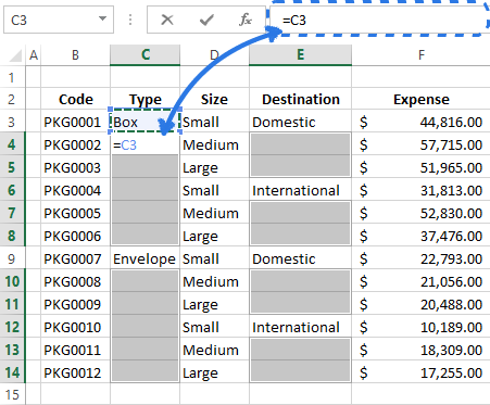
The formula (=C3) shows that cell C4 will get the value from cell C3.
Here you are! Now each selected cell has a reference to the cell over it.
Note. You should remember that all cells that used to be blank contain formulas now. And if you want to keep your table in order, it’s better to change these formulas to values. Otherwise, you’ll end up with a mess while sorting or updating the table. Read our previous blog post and find out two fastest ways to replace formulas in Excel cells with their values.
Use the Fill Blank Cells add-in by Ablebits
If you don’t want to deal with formulas every time you fill in blanks with cell above or below, you can use a very helpful add-in for Excel created by Ablebits developers. The Fill Blank Cells utility automatically copies the value from the first populated cell downwards or upwards. Keep on reading and find out how it works.
- Download the add-in and install it on your computer.
After the installation the new Ablebits Utilities tab appears in your Excel.
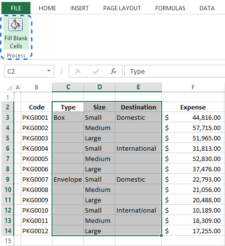
The add-in window displays on the screen with all the selected columns checked. ![]()
If you want to fill the blanks with the value from the cell above, choose the Fill cells downwards option. If you want to copy the content from the cell below, then select Fill cells upwards.

Done! 🙂 ![]()
Besides filling empty cells, this tool will also split merged cells if there are any in your worksheet and indicate table headers.
Check it out! Download the fully-functional trial version of the Fill Blank Cells add-in and see how it can save you much time and effort.
Fill empty cells with 0 or another specific value
What if you need to fill all the blanks in your table with zero, or any other number or a specific text? Here are two ways to solve this problem.
Method 1
- Select the empty cells.
- Press F2 to enter a value in the active cell.
- Type in the number or text you want.
- Press Ctrl + Enter .

A few seconds and you have all the empty cells filled with the value you entered.
Method 2
- Select the range with empty cells.
- Press Ctrl + H to display the Find & Replace dialog box.
- Move to the Replace tab in the dialog.
- Leave the Find what field blank and enter the necessary value in the Replace with text box.
- Click Replace All.


It will automatically fill in the blank cells with the value you entered in the Replace with text box.
Whichever way you choose, it will take you a minute to complete your Excel table.
Now you know the tricks for filling in blanks with different values in Excel 2013. I am sure it will be no sweat for you to do it using a simple formula, Excel’s Find & Replace feature or user-friendly Ablebits add-in.
Источник
See all How-To Articles
In this tutorial, you will learn how to find blank cells in Excel and Google Sheets.
Find & Select Empty Cells
There is an easy way to select all the blank cells in any selected range in Excel. Although this method won’t show you the number of blank cells, it will highlight all of them so you can easily locate them in a spreadsheet.
1. First, select the entire data range. Then in the Ribbon, go to Home > Find & Select > Go To Special.
2. In Go To Special dialog window click on Blanks and when done press OK.
As a result, all blank cells are selected.
With this method, you won’t find pseudo-blank cells (cells with formulas that return blanks and cells containing only spaces).
Other ways to identify blanks:
- IsEmpty Function in VBA
- How to use the ISBLANK Function
Find Blank Cells in Google Sheets
Unlike Excel, Google Sheets doesn’t have a Go To Special feature. But you can identify blank cells and select them one-by-one, highlight them, or replace them.
Skip to content
![]()
 When you work with data, you often want to select certain cells, for example all blank cells. You might want to fill them or just mark them. In this article we’ll learn how to select all empty cells.
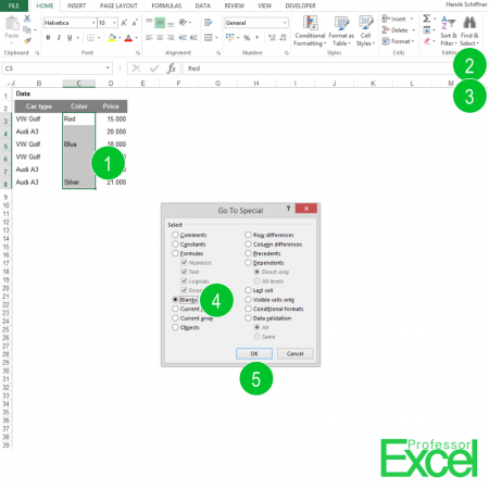
Using “Go To Special” could be helpful:
- Select the range of cells you want to work with, also cells with content.
- Go to “Find & Select” in the Home ribbon.
- Click on “Go To Special”.
- Select “Blanks”.
- Click “OK”.
Now, you can work with all the empty cells at the same time as they are marked. If you want to fill them with text – let’s say “Empty Cell”, type “Empty Cell”. Instead of just pressing Enter, press “Ctrl + Enter”. Now all previously empty cells show the text “Empty Cell”.
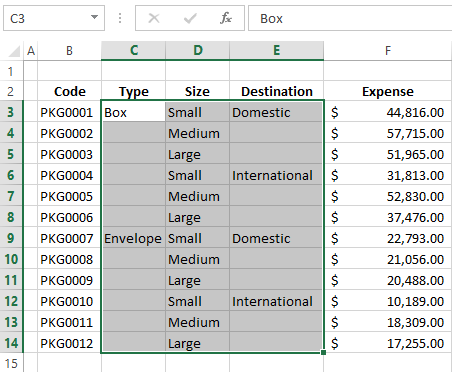
Example: How to fill each empty cell with the content from the next not blank cell above
Let’s have a look at an example: Oftentimes, you got a column of data as shown in the picture above. In column C you can see the color of cars. Now we want to copy the color from the next filled cell above to each blank cell below so that it says ‘Red’ in cell C4; C5 should stay with blue whereas C6 and C7 should say Blue as well.
- First, we need some preparation: Write this formula in cell E2: ‘=E1’ and copy it. You can do this with any cell but it should link to the cell above.
- Follow the steps 1-5 as described. Make sure that cell E2 is still copied.
- After you are done with steps 1-5, cells C4 and C6:C7 should be selected.
- Press paste (Ctrl + v).

Henrik Schiffner is a freelance business consultant and software developer. He lives and works in Hamburg, Germany. Besides being an Excel enthusiast he loves photography and sports.
We use cookies on our website to give you the most relevant experience by remembering your preferences and repeat visits. By clicking “Accept”, you consent to the use of ALL the cookies.
.
In an Excel worksheet, if data is entered in nonadjacent cells, you may discover it a bit troublesome to select and copy the data in non-blank cells. Now, in this post, we will introduce 2 ways to quickly select all non-blank cells.
Excel users are frequently required to copy and paste data. However, sometimes, there may be some troubles. For example, there are multiple discontinuous blank cells in an Excel worksheet. In this case, it is a bit hard to select all the cells which have content. But, don’t worry. Here we will share you 2 approaches to select all non-blank cells in an Excel sheet.
Method 1: Select via “Go To Special”
- At the outset, open the Excel worksheet.
- Then, press “F5” to trigger “Go To” dialog box.

- In the “Go To” dialog, click “Special” button.
- Next, check the “Constants” option and then “Numbers”, “Text”, “Logicals” and “Errors” options.

- Finally, click “OK”.
- When dialog box closes, as you see, all non-blank cells have been selected.


Method 2: Select with Excel VBA
- First off, get access to Excel VBA editor with reference to “How to Run VBA Code in Your Excel“.
- Then, put the following code into an unused module.
Sub SelectAllNonBlankCells()
    Dim objUsedRange As Range
    Dim objRange As Range
    Dim objNonblankRange As Range

    Set objUsedRange = Application.ActiveSheet.UsedRange

    For Each objRange In objUsedRange
        If Not (objRange.Value = "") Then
           If objNonblankRange Is Nothing Then
              Set objNonblankRange = objRange
           Else
              Set objNonblankRange = Application.Union(objNonblankRange, objRange)
           End If
        End If
    Next

    If Not (objNonblankRange Is Nothing) Then
       objNonblankRange.Select
    End If
End Sub

- After that, exit the VBA editor and add this macro to Quick Access Toolbar.
- Now, open your desired worksheet and click the macro button.
- At once, all non-blank cells will be selected, as shown in the following image.


Comparison
| Advantages | Disadvantages | |
| Method 1 | Easy to operate | Users have to manually open “Go To” dialog box and check options every time when they need to select non-blank cells |
| Method 2 | Easy and convenient for reuse | Arise the dangers of external malicious macros |
Repair Annoying Excel Troubles
Excel file is prone to errors and corruption. For instance, if MS Excel is frequently closed improperly, the file can get damaged with ease. Hence, users have to make some precautions, including backing up the files on a periodical basis. In addition, a proficient, robust and reliable xlsx fix tool, like DataNumen Excel Repair, is a matter of necessity.
Author Introduction:
Shirley Zhang is a data recovery expert in DataNumen, Inc., which is the world leader in data recovery technologies, including SQL Server recovery and outlook repair software products. For more information visit www.datanumen.com
A lot of times I work with data that has blank cells in it. If not handled, this could create havoc when these blank cells are referenced in formulas. I usually fill these blank cells with 0 or NA (Not Available).
In huge data sets, it is practically impossible (or highly inefficient) to do this manually. Thankfully, there is a way to select blank cells in Excel in one go.
Select Blank Cells in Excel
Here is how you can Select blank cells in Excel:
- Select the entire data set (including blank cells)
- Press F5 (this opens the Go To dialogue box)
- Click the Special.. button (this opens the Go To special dialogue box)

- Select Blanks and click Ok (this selects all the blank cells in your dataset)

- Type 0 or NA (or whatever you want to type in all the blank cell)
- Press Control + Enter (keep the Control key pressed and then hit Enter)
- Pat your back. It’s done 🙂
You May Also Like the Following Excel Tutorials:
- Select Visible Cells in Excel
- How to Select Non-adjacent cells in Excel?
- How to Deselect Cells in Excel
- How to Move Rows and Columns in Excel.
- How to Select Every Third Row in Excel (or select every Nth Row).
- How to Select 500 cells/rows in Excel (with a single click)
- Fill Down Blank Cells Until the Next Value in Excel (Formula, VBA, Power Query)
- How to Select Entire Column in Excel
- Select Every Other Row in Excel