
Содержание
- Select data for a chart
- Arrange data for charts
- See Also
- Arrange data for charts
- Need more help?
- Quickest Way to Select and Align Charts for an Excel Dashboard
- The Breakdown
- Step-by-Step
- 1) Select Multiple Charts
- 2) Size Multiple Charts
- 3) Select Top Row and Align Top
- 4) Select Edge Charts and Align Left
- Video Demonstration
- Sample File Download
- Create a chart from start to finish
- Create a chart
- Add a trendline
- See also
- Create a chart
- Available chart types
- Add or edit a chart title
- Add axis titles to improve chart readability
- Change the axis labels
- Remove the axis labels
- Need more help?
Select data for a chart
To create a chart, you need to select at least one cell in a range of data (a set of cells). Do one of the following:
If your chart data is in a continuous range of cells, select any cell in that range. Your chart will include all the data in the range.
If your data isn’t in a continuous range, select nonadjacent cells or ranges. Just make sure your selection forms a rectangle.
Tip: If you don’t want to include specific rows or columns of data in a chart, you can simply hide them on the worksheet, or you can apply chart filters to show the data points you want after you create the chart.
Arrange data for charts
Excel can recommend charts for you. The charts it suggests depend on how you’ve arranged the data in your worksheet. You also may have your own charts in mind. Either way, this table lists the best ways to arrange your data for a given chart.
Arrange the data
Column, bar, line, area, surface, or radar chart
Learn more abut
In columns or rows.
This chart uses one set of values (called a data series).
Learn more about
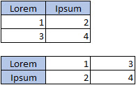
In one column or row, and one column or row of labels.
This chart can use one or more data series.
Learn more about
In one or multiple columns or rows of data, and one column or row of labels.
XY (scatter) or bubble chart
Learn more about
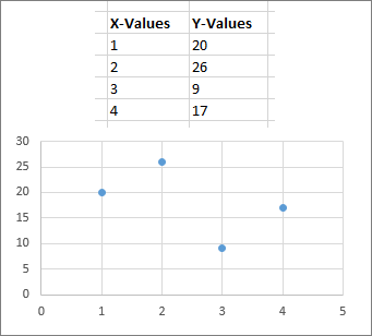
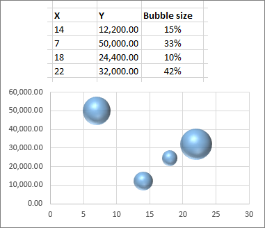
In columns, placing your x values in the first column and your y values in the next column.
For bubble charts, add a third column to specify the size of the bubbles it shows, to represent the data points in the data series.
Learn more about
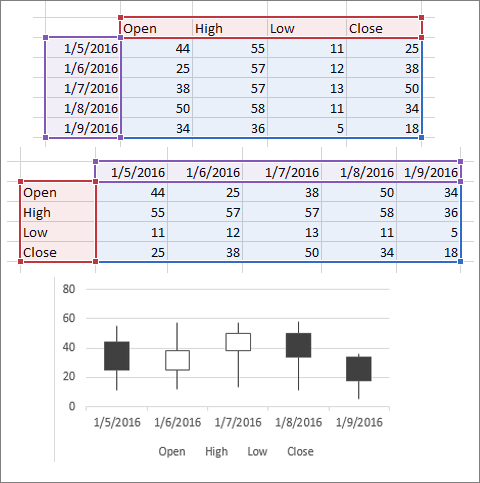
In columns or rows, using a combination of opening, high, low, and closing values, plus names or dates as labels in the right order.
See Also
To create a chart in Excel for the web, you need to select at least one cell in a range of data (a set of cells). Your chart will include all data in that range.
Arrange data for charts
This table lists the best ways to arrange your data for a given chart.
Arrange the data
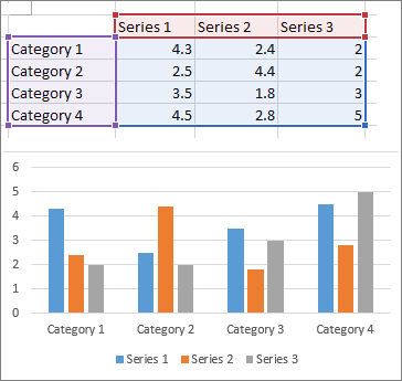
Column, bar, line, area, or radar chart
In columns or rows, like this:
This chart uses one set of values (called a data series).
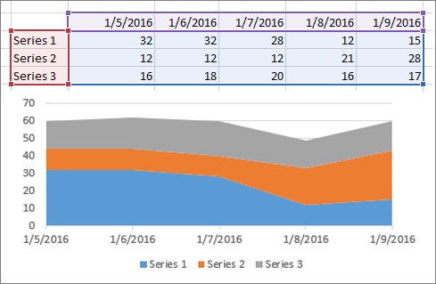
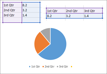
In one column or row, and one column or row of labels, like this:
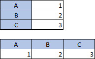
This chart can use one or more data series
In multiple columns or rows of data, and one column or row of labels, like this:
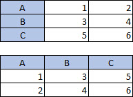
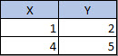
In columns, placing your x values in the first column and your y values in the next column, like this:
For more information about any of these charts, see Available chart types.
Need more help?
You can always ask an expert in the Excel Tech Community or get support in the Answers community.
Источник
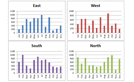
Quickest Way to Select and Align Charts for an Excel Dashboard
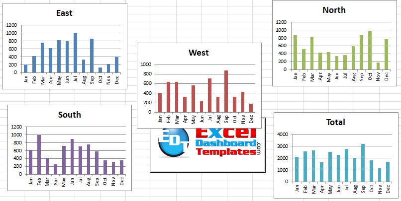
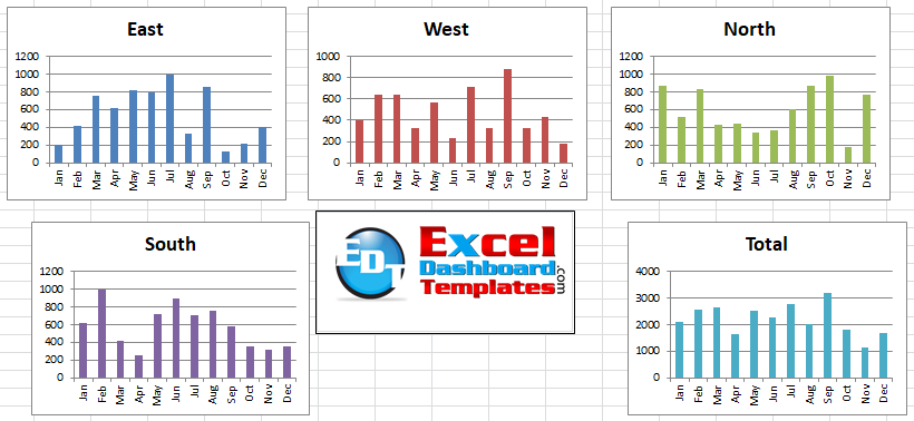
Creating dashboards can take a lot of time.В With this simple technique that I just learned, you can quickly select and align charts for your final Excel Dashboard presentation.
 Quickest Way to Select and Align Charts for an Excel Dashboard Featured Image
The Breakdown
1) Select Multiple Charts
2) Size Multiple Charts
3) Select Top Row and Align Top
4) Select Edge Charts and Align Left
Step-by-Step
1) Select Multiple Charts
Did you know that you can select all of your charts with a Keyboard Shortcut?В This step combined with Step 2 is what will save you all the time in creating your Excel dashboard.
Why is this important? Because you can quickly select all of your charts and then resize them to create a sharp looking presentation.
So tell me the keyboard shortcut already!
First, you must select a chart, any chart, in the Chart Area.В This is typically found in the white space of the chart.В Don’t select any data series, any axis, the title or legend of the chart as this will stop the technique from working.
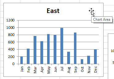 Select Chart Area
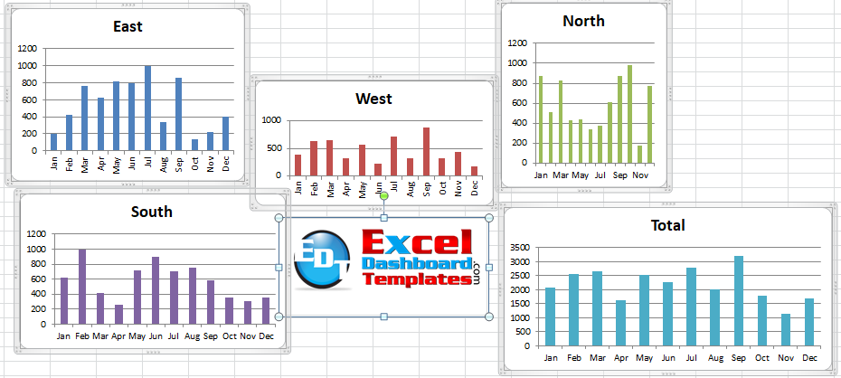
Second, press CTRL+A to select all to select all of your charts on the active worksheet.
 CTRL + A to Select All Charts
NOTE: This will not only select every chart, it will also select every picture on your worksheet.
Finally, if you have selected any chart or picture that do not want to have in the selection, simply hold down either the SHIFT or CTRL key and left click on the chart or picture you want to remove from the mass selection.В For instance, I had an image on my worksheet that was selected, so I can keep the rest selected and un-select the image as you see here:
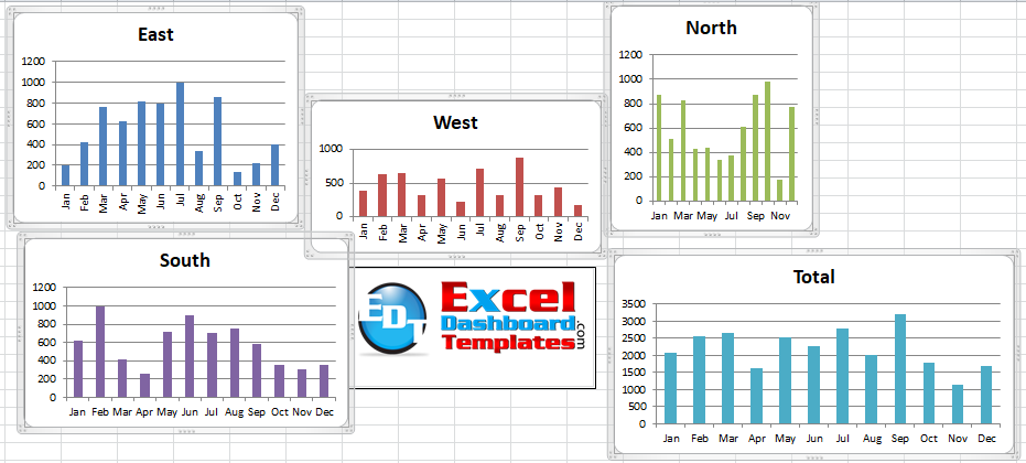 Hold Shift or CTRL and Left click on Object to Un-Select
2) Size Multiple Charts
Now that the dashboard charts are selected on the worksheet, we need to get them all to look the same.
In order to do this, we can use the Ribbon and Size controls.
You will find these controls in the Drawing Tools > Format Ribbon.
NOTE: You will ONLY see these controls when you have at least one chart selected.
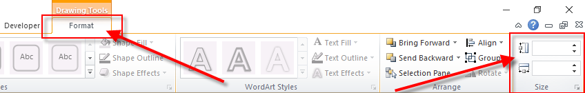 Format Ribbon – Size Controls
Just fill in the Height and press enter in the upper size control and then fill in the Width and press enter.В For my sample chart, I am using 2.25 and3.25
Your charts should now look like this:
 Resized Charts to Same Size
3) Select Top Row and Align Top
Now that the charts are all the same size, we need to get them into the right position.В To do this, first, unselect the charts by clicking anywhere in the worksheet.В Then select the charts you want on the top of the dashboard by holding down either the Shift or CTRL key and then use your mouse to left click on each graph.
Now that you have the charts selected, click on the Drawing Tools > Format Ribbon and then click on the Align button.
Format Ribbon – Align Button
Complete the action by choosing Align Top from the Align Drop Down Menu.
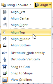 Align Top Menu Selection
Your Excel dashboard chars should now look like this:
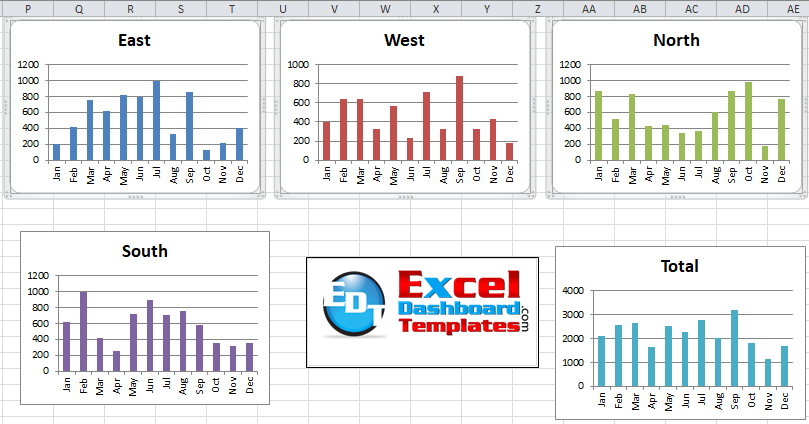 Excel Dashboard Top Alignment
Final action would be with the charts selected to move them to the final location you want.В I want my Excel Dashboard charts positioned around the logo, so it may look a little strange at this stage.
 Excel Dashboard Top Alignment Re-positioned
Repeat these same steps of selecting the bottom charts and Align Top.В However, when I re-position the lower charts, I will put them slightly left of the upper row alignment.В That way I can get these charts aligned properly with the next step.В My Dashboard now looks like this:
 Excel Dashboard Bottom Row Top Alignment Re-positioned
4) Select Edge Charts and Align Left
This step is very similar to the previous one, but it only deals with the edges.В So for thisВ example, I mean aligning the 2 left charts and then the 2 rightmost charts.
For either the left of the right sides, first, select the charts using your left mouse button while holding down the SHIFT or CTRL button.
ThenВ click on the Drawing Tools > Format Ribbon and then click on the Align button.
Format Ribbon – Align Button
Complete the action by choosing Align Left from the Align Drop Down Menu.
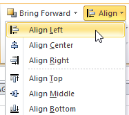 Align Left Menu
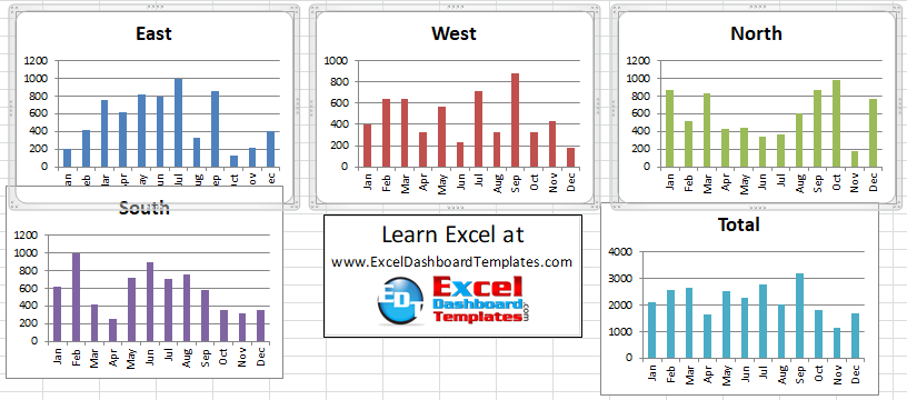
After doing the same action for both charts on the sides, your final Excel Dashboard Layout will look like this:
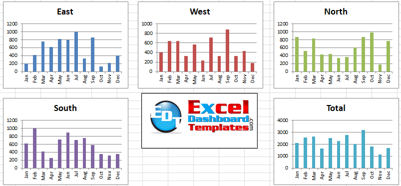 Excel Dashboard Final Size and Alignment
I feel that spending time on the dashboard aesthetics will help your readers focus on the charts and the data versus being distracted by improper sizes and alignments.В If you learn these Excel Dashboard tips and tricks, you will not only save time, you will look like a rockstar to your executives.
Video Demonstration
Check out this Video tutorial on the techniques presented above.
Sample File Download
Did you know about CTRL+A selecting charts only before?В I hadn’t thought about it till just recently.В What is your favorite keyboard shortcut or chart tip/trick?В Let me know in the comments below!
Источник
Create a chart from start to finish
Charts help you visualize your data in a way that creates maximum impact on your audience. Learn to create a chart and add a trendline. You can start your document from a recommended chart or choose one from our collection of pre-built chart templates.

Create a chart
Select data for the chart.
Select Insert > Recommended Charts.
Select a chart on the Recommended Charts tab, to preview the chart.
Note: You can select the data you want in the chart and press ALT + F1 to create a chart immediately, but it might not be the best chart for the data. If you don’t see a chart you like, select the All Charts tab to see all chart types.
Add a trendline
Select Design > Add Chart Element.
Select Trendline and then select the type of trendline you want, such as Linear, Exponential, Linear Forecast, or Moving Average.
Note: Some of the content in this topic may not be applicable to some languages.
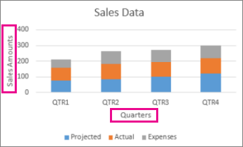
Charts display data in a graphical format that can help you and your audience visualize relationships between data. When you create a chart, you can select from many chart types (for example, a stacked column chart or a 3-D exploded pie chart). After you create a chart, you can customize it by applying chart quick layouts or styles.
Charts contain several elements, such as a title, axis labels, a legend, and gridlines. You can hide or display these elements, and you can also change their location and formatting.
 Chart title
 Plot area
 Legend
 Axis titles
 Axis labels
 Tick marks
 Gridlines
You can create a chart in Excel, Word, and PowerPoint. However, the chart data is entered and saved in an Excel worksheet. If you insert a chart in Word or PowerPoint, a new sheet is opened in Excel. When you save a Word document or PowerPoint presentation that contains a chart, the chart’s underlying Excel data is automatically saved within the Word document or PowerPoint presentation.
Note: The Excel Workbook Gallery replaces the former Chart Wizard. By default, the Excel Workbook Gallery opens when you open Excel. From the gallery, you can browse templates and create a new workbook based on one of them. If you don’t see the Excel Workbook Gallery, on the File menu, click New from Template.
On the View menu, click Print Layout.
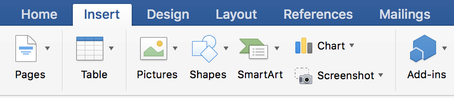
Click the Insert tab, and then click the arrow next to Chart.
Click a chart type, and then double-click the chart you want to add.
When you insert a chart into Word or PowerPoint, an Excel worksheet opens that contains a table of sample data.
In Excel, replace the sample data with the data that you want to plot in the chart. If you already have your data in another table, you can copy the data from that table and then paste it over the sample data. See the following table for guidelines for how to arrange the data to fit your chart type.
For this chart type
Arrange the data
Area, bar, column, doughnut, line, radar, or surface chart
In columns or rows, as in the following examples:
In columns, putting x values in the first column and corresponding y values and bubble size values in adjacent columns, as in the following examples:
In one column or row of data and one column or row of data labels, as in the following examples:
In columns or rows in the following order, using names or dates as labels, as in the following examples:
X Y (scatter) chart
In columns, putting x values in the first column and corresponding y values in adjacent columns, as in the following examples:
To change the number of rows and columns included in the chart, rest the pointer on the lower-right corner of the selected data, and then drag to select additional data. In the following example, the table is expanded to include additional categories and data series.
To see the results of your changes, switch back to Word or PowerPoint.
Note: When you close the Word document or the PowerPoint presentation that contains the chart, the chart’s Excel data table closes automatically.
After you create a chart, you might want to change the way that table rows and columns are plotted in the chart. For example, your first version of a chart might plot the rows of data from the table on the chart’s vertical (value) axis, and the columns of data on the horizontal (category) axis. In the following example, the chart emphasizes sales by instrument.
However, if you want the chart to emphasize the sales by month, you can reverse the way the chart is plotted.
On the View menu, click Print Layout.
Click the chart.
Click the Chart Design tab, and then click Switch Row/Column.
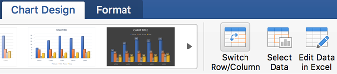
If Switch Row/Column is not available
Switch Row/Column is available only when the chart’s Excel data table is open and only for certain chart types. You can also edit the data by clicking the chart, and then editing the worksheet in Excel.
On the View menu, click Print Layout.
Click the chart.
Click the Chart Design tab, and then click Quick Layout.
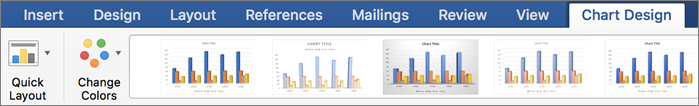
Click the layout you want.
To immediately undo a quick layout that you applied, press  + Z .
+ Z .
Chart styles are a set of complementary colors and effects that you can apply to your chart. When you select a chart style, your changes affect the whole chart.
On the View menu, click Print Layout.
Click the chart.
Click the Chart Design tab, and then click the style you want.
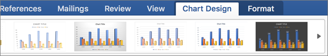
To see more styles, point to a style, and then click  .
.
To immediately undo a style that you applied, press + Z .
On the View menu, click Print Layout.
Click the chart, and then click the Chart Design tab.
Click Add Chart Element.
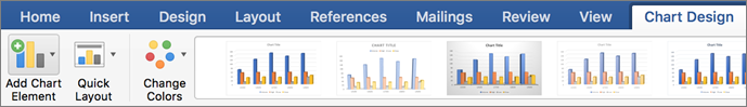
Click Chart Title to choose title format options, and then return to the chart to type a title in the Chart Title box.
See also
Create a chart
You can create a chart for your data in Excel for the web. Depending on the data you have, you can create a column, line, pie, bar, area, scatter, or radar chart.
Click anywhere in the data for which you want to create a chart.
To plot specific data into a chart, you can also select the data.
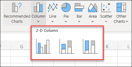
Select Insert > Charts > and the chart type you want.

On the menu that opens, select the option you want. Hover over a chart to learn more about it.
Tip: Your choice isn’t applied until you pick an option from a Charts command menu. Consider reviewing several chart types: as you point to menu items, summaries appear next to them to help you decide.
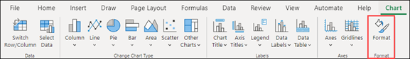
To edit the chart (titles, legends, data labels), select the Chart tab and then select Format.
In the Chart pane, adjust the setting as needed. You can customize settings for the chart’s title, legend, axis titles, series titles, and more.

Available chart types
It’s a good idea to review your data and decide what type of chart would work best. The available types are listed below.
Data that’s arranged in columns or rows on a worksheet can be plotted in a column chart. A column chart typically displays categories along the horizontal axis and values along the vertical axis, like shown in this chart:

Types of column charts
Clustered column A clustered column chart shows values in 2-D columns. Use this chart when you have categories that represent:
Ranges of values (for example, item counts).
Specific scale arrangements (for example, a Likert scale with entries, like strongly agree, agree, neutral, disagree, strongly disagree).
Names that are not in any specific order (for example, item names, geographic names, or the names of people).
Stacked column A stacked column chart shows values in 2-D stacked columns. Use this chart when you have multiple data series and you want to emphasize the total.
100% stacked column A 100% stacked column chart shows values in 2-D columns that are stacked to represent 100%. Use this chart when you have two or more data series and you want to emphasize the contributions to the whole, especially if the total is the same for each category.
Data that is arranged in columns or rows on a worksheet can be plotted in a line chart. In a line chart, category data is distributed evenly along the horizontal axis, and all value data is distributed evenly along the vertical axis. Line charts can show continuous data over time on an evenly scaled axis, and are therefore ideal for showing trends in data at equal intervals, like months, quarters, or fiscal years.

Types of line charts
Line and line with markers Shown with or without markers to indicate individual data values, line charts can show trends over time or evenly spaced categories, especially when you have many data points and the order in which they are presented is important. If there are many categories or the values are approximate, use a line chart without markers.
Stacked line and stacked line with markers Shown with or without markers to indicate individual data values, stacked line charts can show the trend of the contribution of each value over time or evenly spaced categories.
100% stacked line and 100% stacked line with markers Shown with or without markers to indicate individual data values, 100% stacked line charts can show the trend of the percentage each value contributes over time or evenly spaced categories. If there are many categories or the values are approximate, use a 100% stacked line chart without markers.
Line charts work best when you have multiple data series in your chart—if you only have one data series, consider using a scatter chart instead.
Stacked line charts add the data, which might not be the result you want. It might not be easy to see that the lines are stacked, so consider using a different line chart type or a stacked area chart instead.
Data that is arranged in one column or row on a worksheet can be plotted in a pie chart. Pie charts show the size of items in one data series, proportional to the sum of the items. The data points in a pie chart are shown as a percentage of the whole pie.

Consider using a pie chart when:
You have only one data series.
None of the values in your data are negative.
Almost none of the values in your data are zero values.
You have no more than seven categories, all of which represent parts of the whole pie.
Data that is arranged in columns or rows only on a worksheet can be plotted in a doughnut chart. Like a pie chart, a doughnut chart shows the relationship of parts to a whole, but it can contain more than one data series.

Tip: Doughnut charts are not easy to read. You may want to use a stacked column or stacked bar chart instead.
Data that is arranged in columns or rows on a worksheet can be plotted in a bar chart. Bar charts illustrate comparisons among individual items. In a bar chart, the categories are typically organized along the vertical axis, and the values along the horizontal axis.

Consider using a bar chart when:
The axis labels are long.
The values that are shown are durations.
Types of bar charts
Clustered A clustered bar chart shows bars in 2-D format.
Stacked bar Stacked bar charts show the relationship of individual items to the whole in 2-D bars
100% stacked A 100% stacked bar shows 2-D bars that compare the percentage that each value contributes to a total across categories.
Data that is arranged in columns or rows on a worksheet can be plotted in an area chart. Area charts can be used to plot change over time and draw attention to the total value across a trend. By showing the sum of the plotted values, an area chart also shows the relationship of parts to a whole.

Types of area charts
Area Shown in 2-D format, area charts show the trend of values over time or other category data. As a rule, consider using a line chart instead of a non-stacked area chart, because data from one series can be hidden behind data from another series.
Stacked area Stacked area charts show the trend of the contribution of each value over time or other category data in 2-D format.
100% stacked 100% stacked area charts show the trend of the percentage that each value contributes over time or other category data.
Data that is arranged in columns and rows on a worksheet can be plotted in an scatter chart. Place the x values in one row or column, and then enter the corresponding y values in the adjacent rows or columns.
A scatter chart has two value axes: a horizontal (x) and a vertical (y) value axis. It combines x and y values into single data points and shows them in irregular intervals, or clusters. Scatter charts are typically used for showing and comparing numeric values, like scientific, statistical, and engineering data.

Consider using a scatter chart when:
You want to change the scale of the horizontal axis.
You want to make that axis a logarithmic scale.
Values for horizontal axis are not evenly spaced.
There are many data points on the horizontal axis.
You want to adjust the independent axis scales of a scatter chart to reveal more information about data that includes pairs or grouped sets of values.
You want to show similarities between large sets of data instead of differences between data points.
You want to compare many data points without regard to time — the more data that you include in a scatter chart, the better the comparisons you can make.
Types of scatter charts
Scatter This chart shows data points without connecting lines to compare pairs of values.
Scatter with smooth lines and markers and scatter with smooth lines This chart shows a smooth curve that connects the data points. Smooth lines can be shown with or without markers. Use a smooth line without markers if there are many data points.
Scatter with straight lines and markers and scatter with straight lines This chart shows straight connecting lines between data points. Straight lines can be shown with or without markers.
Data that is arranged in columns or rows on a worksheet can be plotted in a radar chart. Radar charts compare the aggregate values of several data series.

Type of radar charts
Radar and radar with markers With or without markers for individual data points, radar charts show changes in values relative to a center point.
Filled radar In a filled radar chart, the area covered by a data series is filled with a color.
Add or edit a chart title
You can add or edit a chart title, customize its look, and include it on the chart.
Click anywhere in the chart to show the Chart tab on the ribbon.
Click Format to open the chart formatting options.
In the Chart pane, expand the Chart Title section.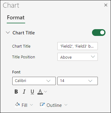
Add or edit the Chart Title to meet your needs.
Use the switch to hide the title if you don’t want your chart to show a title.
Add axis titles to improve chart readability
Adding titles to the horizontal and vertical axes in charts that have axes can make them easier to read. You can’t add axis titles to charts that don’t have axes, such as pie and doughnut charts.
Much like chart titles, axis titles help the people who view the chart understand what the data is about.
Click anywhere in the chart to show the Chart tab on the ribbon.
Click Format to open the chart formatting options.
In the Chart pane, expand the Horizontal Axis or Vertical Axis section.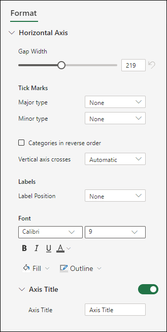
Add or edit the Horizontal Axis or Vertical Axis options to meet your needs.
Expand the Axis Title.
Change the Axis Title and modify the formatting.
Use the switch to show or hide the title.
Change the axis labels
Axis labels are shown below the horizontal axis and next to the vertical axis. Your chart uses text in the source data for these axis labels.

To change the text of the category labels on the horizontal or vertical axis:
Click the cell which has the label text you want to change.
Type the text you want and press Enter.
The axis labels in the chart are automatically updated with the new text.
Tip: Axis labels are different from axis titles you can add to describe what is shown on the axes. Axis titles aren’t automatically shown in a chart.
Remove the axis labels
To remove labels on the horizontal or vertical axis:
Click anywhere in the chart to show the Chart tab on the ribbon.
Click Format to open the chart formatting options.
In the Chart pane, expand the Horizontal Axis or Vertical Axis section.
From the dropdown box for Label Position, select None to prevent the labels from showing on the chart.
Need more help?
You can always ask an expert in the Excel Tech Community or get support in the Answers community.
Источник
If you need to select all objects embedded into the worksheet, e.g., select all charts to adjust their size,
press Ctrl+G and click the Special button or use Ctrl to select objects individually.
On the Home tab, in the Editing group, click Find & Select, and then
click Go To (or press Ctrl+G):

In the Go To dialog box, click the Special button:

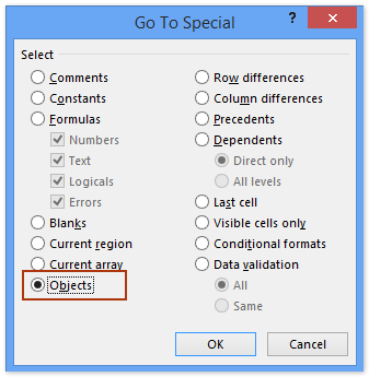
In the Go To Special dialog box, select Objects:

Excel will select all objects on the sheet, not just the charts.
Another option is to select each chart individually. Hold down the Ctrl key and then click all of
your charts to select them. This may be easier if you set the Zoom percent to a small number.
See also this tip in French:
Comment sélectionner tous les graphiques incorporés sur la feuille de calcul.
Please, disable AdBlock and reload the page to continue
Today, 30% of our visitors use Ad-Block to block ads.We understand your pain with ads, but without ads, we won’t be able to provide you with free content soon. If you need our content for work or study, please support our efforts and disable AdBlock for our site. As you will see, we have a lot of helpful information to share.
How do you select all objects, such as all pictures, and all charts? This article is going to introduce tricky ways to select all objects, to select all pictures, and to select all charts easily in active worksheet in Excel.
- Select all objects in active worksheet
- Select all pictures in active worksheet
- Select all charts in active worksheet
- Delete all objects/ pictures/ charts/ shapes in active/selected/all worksheets
Select all objects in active worksheet
You can apply the Go To command to select all objects easily. You can do it with following steps:
Step 1: Press the F5 key to open the Go To dialog box.
Step 2: Click the Special button at the bottom to open the Go To Special dialog box.
Step 3: In the Go To Special dialog box, check the Objects option.

Step 4: Click OK. Then it selects all kinds of objects in active worksheet, including all pictures, all charts, all shapes, and so on.
Easily insert multiple pictures/images into cells in Excel
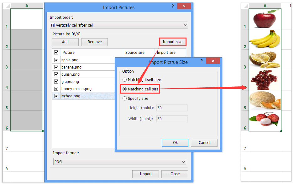
Normally pictures are inserted above cells in Excel. But Kutools for Excel’s Import Pictures utility can help Excel users batch insert each picture/image into a single cell as below screenshot shown.
Kutools for Excel — Includes more than 300 handy tools for Excel. Full feature free trial 30-day, no credit card required! Get It Now
Select all pictures in active worksheet
It seems no easy way to select all pictures except manually selecting each one. Actually, VB macro can help you to select all pictures in active worksheet quickly.
Step 1: Hold down the ALT + F11 keys, and it opens the Microsoft Visual Basic for Applications window.
Step 2: Click Insert > Module, and paste the following macro in the Module Window.
VBA: Select all pictures in active worksheet
Public Sub SelectAllPics()
ActiveSheet.Pictures.Select
End Sub
Step 3: Press the F5 key to run this macro. Then it selects all pictures in active worksheet immediately.
Select all charts in active worksheet
VB macro can also help you to select all charts in active worksheet too.
Step 1: Hold down the ALT + F11 keys, and it opens the Microsoft Visual Basic for Applications window.
Step 2: Click Insert > Module, and paste the following macro in the Module Window.
VBA: Select all charts in active worksheet
Public Sub SelectAllCharts()
ActiveSheet.ChartObjects.Select
End Sub
Step 3: Press the F5 key to run this macro. This macro will select all kinds of charts in active worksheet in a blink of eyes.
Quickly delete all objects/ pictures/ charts/ shapes in active/selected/all worksheets
Sometimes, you may need to delete all pictures, charts, or shapes from current worksheet, current workbook or specified worksheets. You can apply Kutools for Excel’s Delete Illustrations & Objects utility to archive it easily.
Kutools for Excel — Includes more than 300 handy tools for Excel. Full feature free trial 30-day, no credit card required! Get It Now
1. Click Kutools > Delete > Delete Illustrations & Objects.

2. In the opening dialog box, you need to:
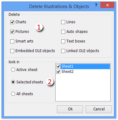
(1) In the Delete section, please specify the types of objects you want to delete.
In our case, we want to remove charts and pictures, therefore we check the Charts option and Pictures option.
(2) In the Look in section, specify the deleting scope.
In our case, we want to remove charts and pictures from several specified sheets, therefore we check the Selected Sheets option, and then check the specified worksheet in the right box. See left screenshot:
Kutools for Excel — Includes more than 300 handy tools for Excel. Full feature free trial 30-day, no credit card required! Get It Now
3. Click the Ok button.
Then all charts and pictures are removed from the specified worksheets.
Demo: delete all objects (pictures and charts) easily in Excel
Kutools for Excel includes more than 300 handy tools for Excel, free to try without limitation in 30 days. Download and Free Trial Now!
Related Articles
The Best Office Productivity Tools
Kutools for Excel Solves Most of Your Problems, and Increases Your Productivity by 80%
- Reuse: Quickly insert complex formulas, charts and anything that you have used before; Encrypt Cells with password; Create Mailing List and send emails…
- Super Formula Bar (easily edit multiple lines of text and formula); Reading Layout (easily read and edit large numbers of cells); Paste to Filtered Range…
- Merge Cells/Rows/Columns without losing Data; Split Cells Content; Combine Duplicate Rows/Columns… Prevent Duplicate Cells; Compare Ranges…
- Select Duplicate or Unique Rows; Select Blank Rows (all cells are empty); Super Find and Fuzzy Find in Many Workbooks; Random Select…
- Exact Copy Multiple Cells without changing formula reference; Auto Create References to Multiple Sheets; Insert Bullets, Check Boxes and more…
- Extract Text, Add Text, Remove by Position, Remove Space; Create and Print Paging Subtotals; Convert Between Cells Content and Comments…
- Super Filter (save and apply filter schemes to other sheets); Advanced Sort by month/week/day, frequency and more; Special Filter by bold, italic…
- Combine Workbooks and WorkSheets; Merge Tables based on key columns; Split Data into Multiple Sheets; Batch Convert xls, xlsx and PDF…
- More than 300 powerful features. Supports Office / Excel 2007-2021 and 365. Supports all languages. Easy deploying in your enterprise or organization. Full features 30-day free trial. 60-day money back guarantee.
")
Office Tab Brings Tabbed interface to Office, and Make Your Work Much Easier
- Enable tabbed editing and reading in Word, Excel, PowerPoint, Publisher, Access, Visio and Project.
- Open and create multiple documents in new tabs of the same window, rather than in new windows.
- Increases your productivity by 50%, and reduces hundreds of mouse clicks for you every day!
")
Comments (16)
Rated 5 out of 5
·
1 ratings
How to select all objects (pictures and charts) easily in Excel?
How do you select all objects, such as all pictures, and all charts? This article is going to introduce tricky ways to select all objects, to select all pictures, and to select all charts easily in active worksheet in Excel.
Select all objects in active worksheet
Select all pictures in active worksheet
Select all charts in active worksheet
Delete all objects/ pictures/ charts/ shapes in active/selected/all worksheets
Easily insert multiple pictures/images into cells in Excel
Normally pictures are inserted above cells in Excel. But Kutools for Excel’s Import Pictures utility can help Excel users batch insert each picture/image into a single cell as below screenshot shown:
Go to Download Free Trial 60 daysPurchasePayPal / MyCommerce

Recommended Productivity Software
Office Tab: Use tabbed interface in Office as the use of web browser Chrome, Firefox and Internet Explorer.Kutools for Excel: Adds 120 powerful new features to Excel. Increase your productivity in 5 minutes. Save two hours every day!Classic Menu for Office: Brings back your familiar menus to Office 2007, 2010, 2013 and 2016 (includes Office 365).
 Select all objects in active worksheet

Amazing! Using Tabs in Excel like Firefox, Chrome, Internet Explore 10!
How to be more efficient and save time when using Excel?
You can apply the Go To command to select all objects easily. You can do it with following steps:
Step 1: Press the F5 key to open the Go To dialog box.
Step 2: Click the Special button at the bottom to open the Go To Special dialog box.
Step 3: In the Go To Special dialog box, check the Objects option.
Step 4: Click OK. Then it selects all kinds of objects in active worksheet, including all pictures, all charts, all shapes, and so on.
Select all pictures in active worksheet
It seems no easy way to select all pictures except manually selecting each one. Actually, VB macro can help you to select all pictures in active worksheet quickly.
Step 1: Hold down the ALT + F11 keys, and it opens the Microsoft Visual Basic for Applications window.
Step 2: Click Insert > Module, and paste the following macro in the Module Window.
VBA: Select all pictures in active worksheet
1
2
3
Public Sub SelectAllPics()
ActiveSheet.Pictures.Select
End Sub
Step 3: Press the F5 key to run this macro. Then it selects all pictures in active worksheet immediately.
Select all charts in active worksheet
VB macro can also help you to select all charts in active worksheet too.
Step 1: Hold down the ALT + F11 keys, and it opens the Microsoft Visual Basic for Applications window.
Step 2: Click Insert > Module, and paste the following macro in the Module Window.
VBA: Select all charts in active worksheet
1
2
3
Public Sub SelectAllCharts()
ActiveSheet.ChartObjects.Select
End Sub
Step 3: Press the F5 key to run this macro. This macro will select all kinds of charts in active worksheet in a blink of eyes.
 Quickly delete all objects/ pictures/ charts/ shapes in active/selected/all worksheets
Sometimes, you may need to delete all pictures, charts, or shapes from current worksheet, current workbook or specified worksheets. You can apply Kutools for Excel’s Delete Illustrations & Objects utility to archive it easily.
Kutools for Excel — Combines More Than 120 Advanced Functions and Tools for Microsoft Excel
Go to DownloadFree Trial 60 daysPurchasePayPal / MyCommerce
1. Click Kutools > Delete > Delete Illustrations & Objects.
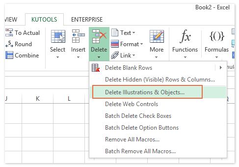
2. In the opening dialog box, you need to:

(1) In the Delete section, please specify the types of objects you want to delete.
In our case, we want to remove charts and pictures, therefore we check the Charts option and Pictures option.
(2) In the Look in section, specify the deleting scope.
In our case, we want to remove charts and pictures from several specified sheets, therefore we check the Selected Sheets option, and then check the specified worksheet in the right box. See left screenshot:
Free Download Kutools for Excel Now
3. Click the Ok button.
Then all charts and pictures are removed from the specified worksheets.
Related Articles
Delete all Pictures easily
Delete all charts Workbooks
Delete all Auto Shapes quickly
Delete all Text Boxes quickly
Is your problem solved?
Yes, I want to be more efficiency and save time when using Excel No, the problem persists and I need further support
Recommended Productivity Tools
The following tools will greatly save your time and effort, which one do you prefer?Office Tab: Using handy tabs in your Office, as the way of Chrome, Firefox and New Internet Explorer.Kutools for Excel: 120 powerful new functions for Excel, Increase your productivity in 5 minutes. Save two hours every day!Classic Menu for Office: Bring back familiar menus to Office 2007, 2010, 2013 and 365, as if it were Office 2000 and 2003.
Kutools for Excel
 Amazing! Increase your productivity in 5 minutes. Don’t need any special skills, save two hours every day!
More than 120 powerful advanced functions which designed for Excel:
- Merge Cell/Rows/Columns without Losing Data.
- Combine and Consolidate Multiple Sheets and Workbooks.
- Compare Ranges, Copy Multiple Ranges, Convert Text to Date, Unit and Currency Conversion.
- Count by Colors, Paging Subtotals, Advanced Sort and Super Filter,
- More Select/Insert/Delete/Text/Format/Link/Comment/Workbooks/Worksheets Tools…

![]()
![]()
![]()
To create a chart, you need to select at least one cell in a range of data (a set of cells). Do one of the following:
-
If your chart data is in a continuous range of cells, select any cell in that range. Your chart will include all the data in the range.
-
If your data isn’t in a continuous range, select nonadjacent cells or ranges. Just make sure your selection forms a rectangle.
Tip: If you don’t want to include specific rows or columns of data in a chart, you can simply hide them on the worksheet, or you can apply chart filters to show the data points you want after you create the chart.
Arrange data for charts
Excel can recommend charts for you. The charts it suggests depend on how you’ve arranged the data in your worksheet. You also may have your own charts in mind. Either way, this table lists the best ways to arrange your data for a given chart.
|
For this chart |
Arrange the data |
|---|---|
|
Column, bar, line, area, surface, or radar chart Learn more abut column, bar, line, area, surface, and radar charts. |
In columns or rows.
|
|
Pie chart This chart uses one set of values (called a data series). Learn more about pie charts. |
In one column or row, and one column or row of labels.
|
|
Doughnut chart This chart can use one or more data series. Learn more about doughnut charts. |
In one or multiple columns or rows of data, and one column or row of labels.
|
|
XY (scatter) or bubble chart Learn more about XY (scatter) charts and bubble charts. |
In columns, placing your x values in the first column and your y values in the next column.
For bubble charts, add a third column to specify the size of the bubbles it shows, to represent the data points in the data series.
|
|
Stock chart Learn more about stock charts. |
In columns or rows, using a combination of opening, high, low, and closing values, plus names or dates as labels in the right order.
|
See Also
Create a chart
Available chart types
Add a data series to your chart
Add or remove a secondary axis in a chart in Excel
Change the data series in a chart
To create a chart in Excel for the web, you need to select at least one cell in a range of data (a set of cells). Your chart will include all data in that range.
Arrange data for charts
This table lists the best ways to arrange your data for a given chart.
|
For this chart |
Arrange the data |
|---|---|
|
Column, bar, line, area, or radar chart |
In columns or rows, like this:
|
|
Pie chart This chart uses one set of values (called a data series). |
In one column or row, and one column or row of labels, like this:
|
|
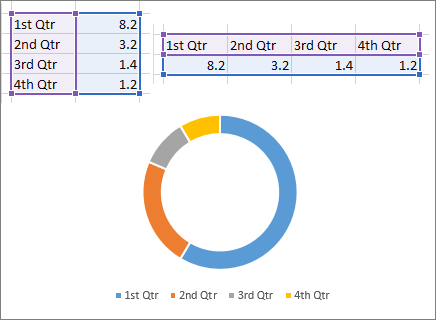
Doughnut chart This chart can use one or more data series |
In multiple columns or rows of data, and one column or row of labels, like this:
|
|
Scatter chart |
In columns, placing your x values in the first column and your y values in the next column, like this:
|
For more information about any of these charts, see Available chart types.