Scroll rows in excel

Bottom Line:  Learn about a new feature update in Excel called Smooth Scrolling which improves the worksheet navigation experience.  I also explain some tips for scrolling and resizing rows and columns on older versions of Excel.

Skill Level: Beginner

Watch the Tutorial

A Welcome Update

Excel just fixed an issue that has been an annoyance to users for more than 35 years! They’ve just rolled out Smooth Scrolling.

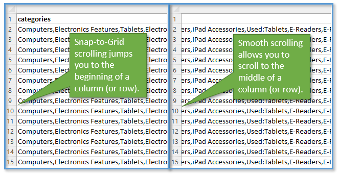
Up until now, when you would scroll either vertically or horizontally, the scrolling would have a snap-to-grid behavior. That means it would always jump to the beginning of a column or row.

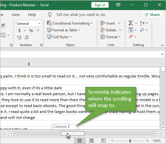
Let’s say you had a column that was extremely wide—wider than the width of your screen. If you were to use the scroll bar at the bottom of the page to move right, you wouldn’t see the scrolling on your screen as you moved along the scroll bar. Instead, there is a screentip telling you where the grid will snap to when you release your mouse.

But with Smooth Scrolling, you can now scroll to any portion of the large column (or row) and the screen will move as you scroll. Then it will remain there when you stop scrolling.

So What’s the Big Deal?

You might be thinking, “Why is this important? Does it really matter?”

It may be a small change, but it alleviates a good amount of frustration. For example, there are times when you might want to compare information in adjacent columns or rows but you simply aren’t able to view both of them at the same time because of their size. Excel will snap you to a place you don’t want to be because of the layout of the grid.

But with Smooth Scrolling, you can drag along the scrollbar with your mouse to exactly what you want to see, and when you take you finger off the mouse button, the screen will remain right where you want it.

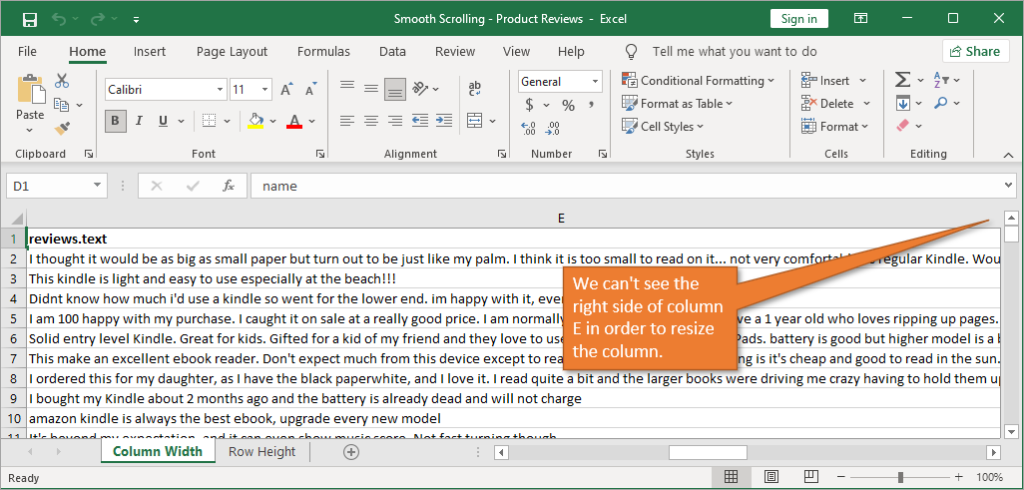
Another annoyance that Smooth Scrolling resolves is in regard to resizing. If a column is larger than my screen width and I want to reduce the size by dragging the right side of the header to the left, I can’t even see the right side of the column when the scrolling snaps me to the left side.

With Smooth Scrolling, that’s not an issue anymore.

Smooth Scrolling is currently only available on the Beta channel for Microsoft 365, and will be released to additional channels in the future. So if you are working an older version of Excel, there are a couple of ways to resize your large columns or rows so that they are more manageable to work with.

Workarounds for Older Versions of Excel

It can be frustrating to not necessarily be able to see the portion of the column that you want to see. It’s even more frustrating on smaller monitors or in smaller windows. The best way to deal with this is to resize the column width (or row height if you are dealing with a row that is too tall).

Here are a couple of ways to do that.

1. Right-click Menu

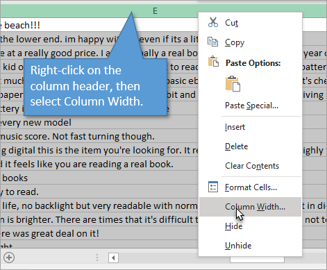
If you right-click on the column header, you will get a menu where you can select Column Width.

This brings up the Column Width window with the current size of the column. You can adjust that number to something smaller. That will resize your column so that the right edge is now visible on your screen.

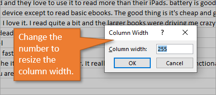
Trivia Fact: 255 is the maximum cell width in Excel.

2. The Zoom Controls

Another option is to use the zoom feature. To zoom in and out, you can hold down the Ctrl key and scroll on your mouse. Or, you can use the zoom controls, found in the bottom-right corner of Excel.

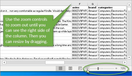
Once you have zoomed out enough, you can resize the column like you normally would, and then you can zoom back in.

Either of these options to resize column widths would also apply to adjusting row heights as well.

A Quick Note

You can also press and release the scroll button on your mouse to create smooth scrolling to the right and left.

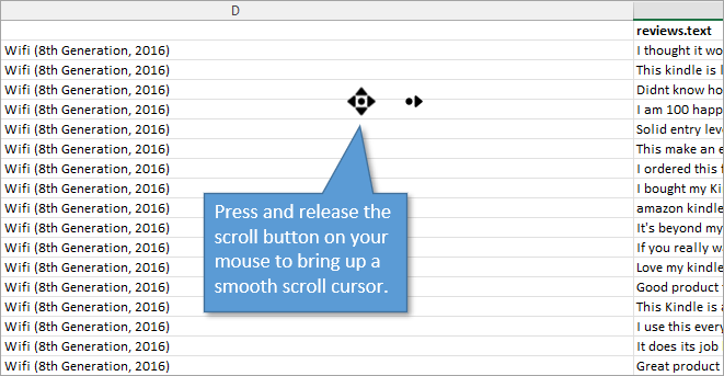
The issue is that when you click the button again, it snaps back to the grid. This is not a method I use very often, but I wanted to make mention of it.

Can I Still Snap to Grid?

The snap-to-grid behavior does still exist in the new version of Excel. You just have to use the arrow buttons instead of dragging the scroll bar.

Conclusion

I’m really happy about this small improvement, and I wonder if you are too. I hope this post is also helpful for anyone who is having trouble resizing their columns or rows in older Excel versions.

Let me know what you think about this updated feature in the comments below!

Press SCROLL LOCK, and then simultaneously hold down CTRL and an arrow key to quickly move through large areas of your worksheet. Note: When SCROLL LOCK is on, Scroll Lock is displayed on the status bar in Excel. Pressing an arrow key while SCROLL LOCK is on will scroll one row up or down or one column left or right.

Why is my Excel sheet not scrolling?

Re: My excel spreadsheet won’t scroll down
You can normally toggle Scroll Lock off and on by hitting the Scroll Lock key on your keyboard. If you don’t have a scroll lock key on your keyboard do this…That should bring up the on-screen keyboard, click on the “scroll lock” key to toggle off that option.

How do I scroll part of an Excel spreadsheet?

Click the View tab on the Ribbon. Select the Freeze Panes command, then choose Freeze Panes from the drop-down menu. The column will be frozen in place, as indicated by the gray line. You can scroll across the worksheet while continuing to view the frozen column on the left.

How do I scroll text in an Excel cell?

On the main worksheet, click-drag the area where you want to place the text box. Ensure Design Mode is enabled and click Properties. Set EnterKeyBehavior, MultiLine, and WordWrap to True. Set ScrollBars to 2 – fmScrollBarsVertical.

How do I unlock scrolling in Excel?

To turn off scroll lock, execute the following step(s).

1. Press the Scroll Lock key (Scroll Lock or ScrLk) on your keyboard.
2. Click Start > Settings > Ease of Access > Keyboard > Use the On-Screen Keyboard (or press the Windows logo key + CTRL + O).
3. Click the ScrLk button.

What key is Scroll Lock?

The Scroll Lock key on a laptop is often a secondary function of another key, located near the Backspace key. If a laptop uses two keys as one key, you must press the Fn key with the second key you want to use. On a laptop, the Scr Lk, Pause, and Break functions are usually part of another key and are in blue text.

Why is Excel scrolling with arrow keys?

When the scroll lock feature is turned on, pressing an arrow key causes Microsoft Excel to move the entire spreadsheet, instead of moving to the next cell. Although helpful for a user viewing a large worksheet, it’s also quite annoying for those who have mistakenly enabled this feature.

How do I unlock Scroll Lock?

Turn off Scroll Lock

1. If your keyboard does not have a Scroll Lock key, on your computer, click Start > Settings > Ease of Access > Keyboard.
2. Click the On Screen Keyboard button to turn it on.
3. When the on-screen keyboard appears on your screen, click the ScrLk button.

How do you scroll with the keyboard?

How to Scroll With a Laptop Keyboard

1. Use the arrow up and arrow down keys. In the lower right side of your keyboard (usually between the letter keys and number keypad) is a set of four arrow keys.
2. Use the page up and page down keys.
3. Use the home and end keys.
4. Scroll numerically.

How do you scroll down on a laptop?

Click the left button under your touch pad. It will click the arrow and make the page move down. Alternatively, you can grab the scroll bar (the gray bar between arrows) by clicking the left button, holding it, then dragging the bar up and down the page.

How do you scroll in Excel without jumping?

Pressing an arrow key while SCROLL LOCK is on will scroll one row up or down or one column left or right. To use the arrow keys to move between cells, you must turn SCROLL LOCK off. To do that, press the Scroll Lock key (labeled as ScrLk) on your keyboard.

How do I scroll using Windows keyboard?

keyboard-scroll

1. alt-up / alt-down to scroll up or down.
2. alt-ctrl-up / alt-ctrl-down to additionally move the cursor.

How do I scroll up?

Here’s how:

1. Using your mouse or laptop track pad, move your cursor to the scroll bar.
2. Then click and hold your mouse; you can now move the scroll bar up and down.
3. Release the mouse button once you reach the place on your screen you would like to go.

What is scroll key in keyboard?

Scroll Lock is a toggling lock key on the keyboard, just like the CAPS LOCK key. Once pressed, Scroll Lock is enabled. To turn it off, simply press the Scroll Lock key again.If Scroll Lock appears, then it’s turned on. To turn it off, just press the Scroll Lock key, which sometimes appears as ScrLk on the keyboard.

How do you scroll down with two fingers?

Enable two-finger scroll via Settings in Windows 10

1. Step 1: Navigate to Settings > Devices > Touchpad.
2. Step 2: In the Scroll and zoom section, select the Drag two fingers to scroll option to turn on the two-finger scroll feature.

How do I scroll down on Windows 10?

How to reverse touchpad scrolling direction on Windows 10

1. Open Settings.
2. Click on Devices.
3. Click on Touchpad. Important: The reverse scrolling option is only available for devices with a precision touchpad.
4. Under the “Scroll and zoom” section, use the drop-down menu to select the Down motion scrolls down option.

How do you scroll in Excel without moving the top row?

Select the cell in the upper-left corner of the range you want to remain scrollable.
To freeze the top row or first column:

1. From the View tab, Windows Group, click the Freeze Panes drop down arrow.
2. Select either Freeze Top Row or Freeze First Column.
3. Excel inserts a thin line to show you where the frozen pane begins.

Can Excel scroll without snapping to cell?

Increase the height on some rows in your spreadsheet and scroll using your mouse wheel or touch pad to see that you can stop partway through a row, and avoid snapping to the top. Drag the scroll bar to see that you can scroll with precision and you can stop anywhere you like.

Watch Video – Creating a Scroll Bar in Excel

A Scroll Bar in Excel is what you need when you have a huge dataset and you don’t want it to hijack your entire screen’s real estate.

It’s a great tool to use in an Excel Dashboard where you have to show a lot of data in a limited space.

In this step-by-step tutorial, I will show you how to create a scroll bar in excel.  You will also learn how to link a dataset to this dynamic scroll bar, such that when a user changes the scroll bar, the data accordingly changes.

Creating a Scroll Bar in Excel

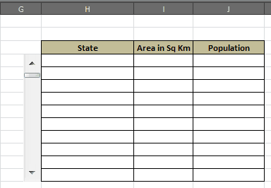
For the purpose of this tutorial, I have taken the data for 28 states in India, along with each state’s area and population (census 2001). Now, I want to create a data set that displays only 10 states at a time, and when the user changes the scroll bar, the data dynamically changes.

Something like this shown below:

Click here to download the example file

Steps to Create a Scroll Bar in Excel

1. The first step is to get your data in place. For the purpose of this post, I have used census 2001 data of 28 Indian States with its Area and Population.
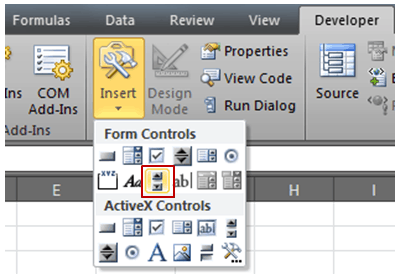
2. Go to Developer Tab –> Insert –> Scroll Bar (Form Control).If you can’t find the developer tab in the ribbon, it is because it has not been enabled. By default, it’s hidden in Excel. You first need to add the developer tab in the ribbon.
3. Click on Scroll Bar (Form Control) button and click anywhere on your worksheet. This will insert a Scroll Bar in the excel worksheet.
4. Right-click on the Scroll Bar and click on ‘Format Control’. This will open a Format Control dialog box.
5. In the Format Control dialogue box go to the ‘Control’ tab, and make the following changes:
   • Current Value: 1
   • Minimum Value: 1
   • Maximum Value: 19 (it is 19 here as we display 10 rows at a time. So when the user makes the scroll bar value 19, it displays rows 19-28)
   • Incremental Change: 1
   • Page Change: 5
   • Cell Link: $L$3
     $L$3 is the cell that is linked to the scroll bar in Excel. Its value varies from 1 to 19. This is the cell value that we use to make the scrollable list. Don’t worry if it doesn’t make sense as of now. Just keep reading and it will become clear!!
6. Resize the Scroll Bar so that it fits the length of the 10 columns (this is just to give it a good look, as shown in the pic below).
7. Now enter the following formula in the first cell (H4) and then copy it to fill all the other cells:
   =OFFSET(C3,$L$3,0)

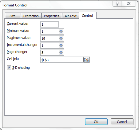
Note that this OFFSET formula is dependent on cell L3, which is linked to the scroll bar.

Now you are all set with a Scroll Bar in Excel.

How does this work?

The OFFSET formula uses cell C3 as the reference cell and offsets it by the values specified by cell L3. Since L3 is linked to scroll bar value, when the scrollbar value becomes 1, the formula refers to the first state name. When it becomes 2, it refers to the second state.

Also, since C3 cell has not been locked, in the second row, the formula becomes =OFFSET(C4,$L$3,0) and works the same way.

Try it yourself.. Download the file

You May Also Like the Following Excel Tutorials:

• Create Dynamic Labels in Scroll Bar in Excel.
• How to Turn OFF Scroll Lock in Excel?
• Adjust Scroll Bar Maximum Value based on a Cell Value in Excel.
• How to Insert and Use a CheckBox in Excel.
• How to Insert and Use Checkmark and Crossmark symbols in Excel.
• How to Insert & Use a Radio Button in Excel.
• Creating Dynamic Filter in Excel.