Save formatting in excel

Home / Advanced Excel / Auto Format Option

Formatting is a tedious task. It’s really hard to format your data whenever you present it to someone. But, this is the only thing that makes your data more meaning full, and easy to consume.

It would be great if you have an option that you can use to format your data without spending much time. So, when it comes to Excel, you have an amazing option that can help you to format your data in no time.

Its name is AUTO FORMAT. In auto-format, you have several pre-designed formats which you can apply to your data instantly.

All you have to do just select a format and click OK to apply. It’s simple and easy. In all the pre-designed formats you have all the important components of formatting, like:

• Number Formatting
• Borders
• Fonts Style
• Patterns and Background Color
• Text Alignment
• Column and Row size

In this post, you will learn about this amazing option that can help you to save a ton of time in the coming days.

Quick Note: It’s one of those Excel Tricks that can help to get better at Basic Excel Skills. So, let’s get started…

Where to Find AUTO FORMAT Option?

If you check Excel 2003 version, the auto- format option is there on the menu. But, with the release of 2007 with ribbon this option is not available in any of the tabs.

That doesn’t mean you can’t use it in earlier versions. It’s still there, but hidden. So, to use it in Excel versions like 2007, 2010, 2013, and 2016 you need to add it to your Excel’s quick access toolbar. It’s a one-time setup so you don’t have to do it again and again.

Add Auto Format on Quick Access Toolbar

To add the auto format to your quick access toolbar please follow these steps.

• First of all, go to your quick access toolbar and click on the small down arrow from the endpoint of the toolbar.

• And, when you click on it, you will get a drop-down menu.

• From this menu, click on “More Commands”.

• Once you click on it, it will open “Customize the Quick Access Toolbar” in the excel options.
• From here, click on the “Choose commands from” drop-down and select “Commands Not in the Ribbon”.

• After that, come to the list of commands you have right below this drop-down.
• And, select the “Auto Format” option and add it to the quick access toolbar.

• Click OK.

Now, you have the auto-format icon in your quick access toolbar.

How to use Auto Format?

Applying formats with an auto-format option is super simple. Let’s say you want to format below data table.

Download this file from here to follow along and follow the below steps to format the table.

• Select any of the cells from your data.

• Go to the quick access toolbar and click on the auto-format button.

• Now, you have a window, where you have different data formats.
• Select one of them and click OK.

• Once you click OK, it will instantly apply your chosen format to the data.

How to Modify a Format in Auto Format

As I mentioned above, all the formats in the auto format are a combination of 6 different components. And you can also add or remove these components from each format before applying them.

Let’s say, you want to add formatting to the below data table but without changing its font style and column width. You need to apply formatting using the below steps.

• Select your data and click on the auto-format button.
• Select a format to apply and click on the “Options” button.
• From options, un-tick “Font” and “Width/Height”.

• And, click OK.

Now, both of the components are not there in your formatting.

Removing Formatting

Well, to remove formatting from data the best way is to use a shortcut key Alt + H + E + F. But you can also use the auto format option to remove formatting from your data.

• Select your entire data and open auto format.
• Go to the last in the format list where you have a “None” format.

• Select it and click OK.

Important Points

1. The auto-format is not able to recognize if you already have some formatting on your data. It will ignore and apply new formatting as per the format you have selected.
2. You need at least 2 cells to apply formatting with the auto-format option.

No one can afford the loss of formatting changes done in the Excel worksheet. But sometimes the situation may arise where Excel won’t save formatting changes and due to this whole data formatting goes off after reopening of the Excel worksheet.

Do you have any idea how to deal with this particular Excel not saving formatting changes issue?

No need to get tensed; as our today’s blog is specifically about this particular issue. So just go through all the fixes to resolve Excel not saving formatting changes issues and also know how to recover lost formatting in Excel.

Reason 1# Restricted File Permissions

When an Excel file is saved, it’s compulsory to have folder access permission in which it is been saved.

• Write permission
• Delete permission
• Modify permission
• Read permission

Reason 2# Third Party Add-Ins

If you are unable to save formatting changes done in Excel then the problem is accused by the third-party add-in. Some third-party software add-ins work smoothly with the existing Excel file. Whereas some start causing issues in saving the Excel file and its formatting changes.

Reason 3# Disk Space

Another reason behind the Excel file won’t save changes issue can be the lack of storage space. So make sure that your disk has enough free space to save the file.

Otherwise, you will receive “disk is full” or Excel file won’t save formatting changes like errors.

Reason 4# File Naming

If you are trying to open or save such a file whose path length is more than 218 characters along with the file name then you may get the following error message:

Filename is not valid

As a result of this, you will also start encountering Excel not saving formatting changes like issues.

Reason 5# Antivirus Software

When you install any antivirus software, it scans the entire file stored on the PC. This scanning process sometimes hinders Excel saving tasks correctly.

In order to make a cross-check whether the anti-virus is conflicting with the Excel program. You need to temporarily deactivate the anti-virus software and then try saving up your Excel file.

Reason 6# File-Sharing

If multiple users work concurrently on the shared workbook then this also generates formatting changes won’t saved in Excel.

You will get this problem because Excel can’t save changes of multiple instances in a single piece of time.

Reason 7# Cannot Access Excel Read-only Document 

Excel 2016 not saving formatting changes error also encounters in Excel read-only file.

It’s all because the reason that owner or administrator of the file hasn’t allowed permission for making any changes in the file. Following reasons are highly responsible for this:

• You open such a file and try saving it.
• Trying to save the file on the network or external drive and all of a sudden connection fails.

How To Fix Excel Not Saving Formatting Changes?

Use the following to resolve Excel won’t save formatting changes. These fixes are really very helpful for format retention mainly when you are trying to keep up the original file formatting.

Fix 1# Date Format Issue In Excel

Your assigned dates are changed to text, number, another date format like MM/DD/YYYY is changed to DD/MM/YYYY or to any other format which Excel fails to recognize.

Here is an example of Excel Date won’t save formatting changes:

Suppose you have entered a date September 6 in your Excel cell and after pressing the enter key, the assigned cell value is been converted to ‘Number.’

This shows that the number format of the cell is not properly synchronized with what users trying to get. The cell is already set with a number format that changes your input data to some numerical value.

How To Fix it?

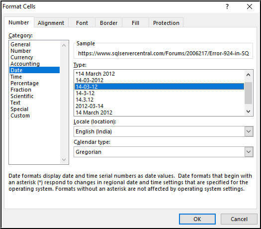
• Make a right-click on the cell having the date; now from the appearing list of options choose Format Cells.
• Go to the “number” tab, after that from the category list choose the “date” and then from the type box choose the date format as per your choice.

Fix 2# Number Format Issue

Excel won’t save formatting changes also arise when Excel number is changed to Date, Text, or any other format which is not well supported.

How To Fix?

 To fix such issues, users need to use the fixes like Paste Special or Error Checking.

• Hit the cell and go to the Home tab from the Excel ribbon. After that click the down-arrow sign present in the number section.
• Here you will see the number format list along with the data present for each of the formats.

Fix 3# Clear Conditional Formatting

Many a time it happens that Excel freezes while working and doesn’t allow you to save your work in that case clearing the conditional formatting is the best option. Below are the steps that are given to perform conditional formatting:

• Open Excel workbook.
• Click on Home>conditional formatting>clear rules>clear rules from an entire sheet

• At the bottom of the Excel sheet select any extra tab and redo the first step.
• Now, select file>save as.
• Make a copy of that spreadsheet in new.

If still, Excel won’t allow you to save formatting changes then apply the conditional formatting again.

Fix 4# Make A Fresh Start

Usually, these kinds of issues are generated when the user tries to open Excel file of one system onto another. Or, when the new PC executes the older version of the Excel application.

How To Fix?

In that case, you need to save your Excel files in widely accepted or native format but not in the older format. Well, you can easily do this by using the ‘Save As’ feature for saving up the Excel file.

Apart from this, Excel won’t save formatting changes can also be fixed by transferring data from the current workbook to the new workbook.

Fix 5# Excel XLS or XLSX file corruption

Chances are also high that just because of the xls/xlsx file corruption your Excel won’t save formatting changes.

To repair corrupt Excel file, you can either use the inbuilt ‘Open or Repair’ tool or you can go with the Excel repair software.

This software repair very efficiently repairs the damaged Excel file in just 3 simple steps, i.e Select, Scan, and Save. Just save the repaired file either on the desired or default location.

* Free version of the product only previews recoverable data.

Using this advanced Excel repair tool you can fix the corruption issue and recover lost formatting in Excel. With this tool, you can easily recover conditional formatting, Chart, table formatting, and all your data formatting completely intact meanwhile Excel file restoring.

Fix 6# Shift Original Worksheets To New One

• Just add a filler worksheet in your Excel workbook. For this, you need to press Shift+F11 from your keyboard.

Note

Well, this sheet is compulsory to have because hen all the relevant data sheets are removed then this sheet will remain.

• Now you need to group all the worksheets excluding the filler one. For this, choose the first datasheet, and press the shift key. After that choose the very ending datasheet.
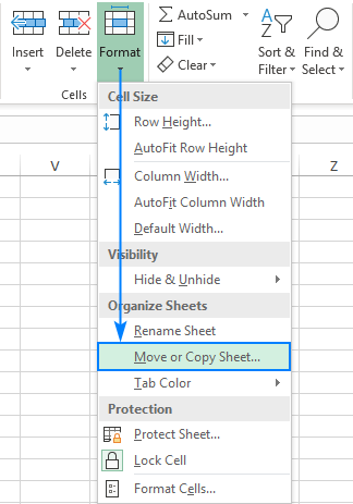
• Make a right-click over the grouped sheets and choose the option “Move or copy”.

• From the To Book list, choose the (New Book).
• Hit the OK button.

 Note:

This step will move your grouped or active worksheets to the new ones.

If your Excel workbook is having VBA macros then you need to manually copy the modules from the old to a new workbook.

Fix 7# Save The File As A Different Excel File Type

• Go to the File menu and choose Save As option.

• From the Save as Type list, choose the file format instead of the current file format.

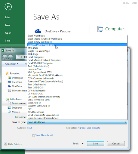
If you are running Excel 2007 or a later version then save the Excel file in .xlsm or .xlsx format rather than .xls.

Fix 8# Save The Workbook To Another Location

Sometimes location at which you are saving the file also leads to generate Excel file won’t save changes like issues.

 So try to save your Excel file in another location like a network drive, removable drive, or local hard disk.

Fix 9# Save New Workbook In The Original Location

If you need to save a new Excel file to the original location then follow down these steps:

• Make an Excel workbook.
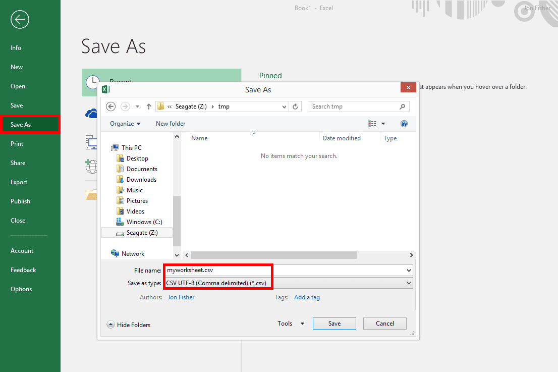
• Go to the File menu and choose the Save As option.

• This will open the Save As dialog box, where you need to perform the following steps.
• Under this Save in the dialog box, choose the location where the original Excel workbook been saved.
• In the box of “File name” assign the name for your new file.
• Hit the Save button.

Fix 10# Save Workbook In Safe Mode

Run your Windows in the safe mode and after that save the Excel workbook on the local hard drive.

If you are using a network location for saving up the Excel workbook, then restart the Windows PC in safe mode along with the network support.  After that try saving the Excel workbook.

Wrap Up:

Hopefully, you have found this article informative and from now onwards you don’t need to deal with this Excel 2016 not saving formatting changes issue.

Apart from this if you have any further queries to ask then let me know by commenting on this post.

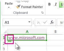
Sometimes when you’re entering information into a worksheet, Excel automatically formats it in a way you didn’t intend. For example, if you type a web address, Excel will turn it into a hyperlink. This can be really helpful, but there might be times when that’s not what you want. In that case, you can turn off automatic formatting for one cell or your whole workbook.

1. Move your mouse pointer over the text that was just automatically formatted, and then click the AutoCorrect Options button that appears. This button is tiny, so look closely as you move the mouse pointer.

1. To remove the formatting for just the text you’ve selected, click Undo. For example, if Excel automatically created a hyperlink and you want to remove it, click Undo Hyperlink.

2. To tell Excel to stop applying this particular type of formatting to your workbook, click Stop. For example, if Excel automatically created a hyperlink and you want to prevent Excel from doing that for the rest of the worksheet, click Stop Automatically Creating Hyperlinks.

Set all automatic formatting options at once

If you want to review and change automatic formatting options all at once, you can do that in the AutoCorrect dialog box.

1. Click File > Options.

2. In the Excel Options box, click Proofing > AutoCorrect Options.

3. On the AutoFormat As You Type tab, check the boxes for the auto formatting you want to use.

   • 
     Internet and network paths with hyperlinks
        : Replaces typed URLs, network paths, and email addresses with hyperlinks.

   • 
     Include new rows and columns in table
        : When you enter data below or next to an Excel table, it expands the table to include the new data. For example, if you have a table in columns A and B, and you enter data in column C, Excel will automatically format column C as part of your table.

   • 
     Fill formulas in tables to create calculated columns
        : Applies one formula to all cells in an Excel table column.

Note: If you want to set how numbers and dates appear, you do that on the Home tab in the Number group. It isn’t part of automatic formatting.

This feature is not available in Excel for the web.

If you have the Excel desktop application, you can use the Open in Excel button to open the workbook and undo automatic formatting.

When working with data in Excel, you will often format data (such as color the cells or make them bold or give a border), to make these stand out.

And if you have to do this for many cells or range of cells, instead of doing it manually, you can do it once and then copy and paste the formatting.

In this tutorial, I will show you how to copy formatting in Excel. You can easily do it by using the Format painter option, using the Fill handle, or Paste special.

Copy the Formatting to a Single Cell

We’ll first see how to copy a formatting to a single cell in Excel. Let’s say that you have cell A2 formatted as an accounting number, with red background and white font color. 

In Cell C2 we have the plain number without any format.

1. Select a formatted cell that has the formatting that you want to copy (A2 in our example)
2. Click on Format Painter in the Home tab. This will change the cursor into a paintbrush with a plus icon

1. Click on a cell where you want to copy a format (C2)

Whenever you select a cell and choose Format Painter in the toolbar, the mouse cursor turns into a white cross with a brush.

This is how you know that the formatting is copied to the clipboard and you can paste it where you want.

Just the way we copied the formatting from one to another in the same sheet. you can also copy formatting to another sheet or another workbook. Simply select the cell from where you want to copy the formatting, enable format painter, select the sheet/workbook where you want to paste it, and select the cells in the destination sheet.

With Format Painter, you can easily copy the following formatting:

• Cell background-color
• Font size and color
• Font (including number format)
• Font characteristics (bold, italics, underline)
• Text alignment and orientation
• Cell borders (type, size, color)
• Custom Number Formatting
• Conditional Formatting

Personally. I find it a huge time saver to copy conditional formatting from one cell to another in the same sheet or other sheets. Excel is smart enough to adjust the rules in conditional formatting in case you’re using custom formulas.

Copy the Formatting to a Range of Cells

Just like you can copy the formatting from one cell to another cell, you can also copy it to a range of cells.

In this case, you need to select a range of cells on which you want to apply the format painter.

Suppose you have a dataset as shown below where you want to copy the formatting from cell A2 to the range of cells in C2:C7

1. Select a formatted cell (A2)
2. Click on Format Painter in the Home tab
3. Select a range of cells where you want to copy a format (C2:C7)

As a result, the format from A2 is copied to the selected range.

PRO TIP: When you click on the Format Paint icon, it allows you to format a cell or range of cells only once. Once you’re done, it’s disabled. So if you want to copy formatting to two ranges of cells, you will have to enable format painter twice. Alternatively, when you double-click on the Format Paint icon, it remains enabled and you can copy formatting to multiple cells or ranges.

Copy the Formatting Using Paste Special

When you copy and paste cells in Excel, you noticed that there are usually multiple paste options, such as: Paste text, Paste values, etc. 

One of these options is Paste formatting. 

This allows you to copy only the formatting from cells to cells.

1. Select and right-click a cell from which you want to copy the formatting (A2)
2. Click Copy (or use the keyboard shortcut CTRL+C).

1. Select a range of cells to which you want to copy the formatting (C2:C7);
2. Right-click anywhere in the selected range;
3. Click the arrow next to Paste Special;
4. Choose the icon for formatting.

The result is the same as using the Format painter.

You can also notice that all formatting that you copied by Format painter is also copied using the Paste special option.

Just like format painter, you can also use the Paste Special technique to paste formatting on the cells or range of cells in the same sheet or other sheet/workbook.

Pro Tip: If you have to copy the formatting from a cell to multiple cells that are scattered through the worksheet, you can use the paste special technique to copy formatting to one cell, and then repeat the process by using the F4 key. So copy the formatting once, then select another cell and press F4, and it will repeat your last action (which was to paste the formatting).

Also read: How to Copy and Paste in Excel Without Changing the Format?

Copy the Formatting Using the Fill Handle

As you probably already know, the fill handle is the little black cross that appears when you position a cursor in the right bottom corner of the cell (as shown below).

This cursor allows you to copy a cell (or range of cells) down the rows.

Apart from copying the cell values, the fill handle also allows you to copy the formatting.

Let’s say that you have a list of numbers in column A, where the first value in the list (A2) is formatted, while other values (A3:A7) are not formatted at all.

What I want is to copy the formatting from cell A2 to all the cells below it.

Below are the steps to do this:

1. Position the cursor in the right bottom corner of a cell from which you want to copy the formatting (A2) until the black cross (fill handle) appears;

1. Drag the fill handle down to the end of the range which we want to format (A7). If you want to copy the cell to the end of the range (until the first blank cell in the range), just double-click the fill handle.

1. When you drop the cursor, by default both value and formatting will be copied to the range. Now, you need to click on the AutoFill Options icon next to the end of the range and choose Fill Formatting Only.

Now, you can see that values are not changed, while the formatting is copied to the whole range.

While I have shown how to use the Fill Handle to copy formatting for one column only, you can use it the same way for the data in a row of data that spans across multiple rows and columns.

One drawback of using the fill handle is that your data needs to be in the same column or row where you have the cell from which you are copying the formatting.  This also means that you cannot use this method to copy the formatting to cells or range of cells that are in another sheet or workbook.

So these are some of the methods you can use to copy formatting from one cell to another cell or range of cells in Excel.

I hope you found this tutorial useful!

Other Excel tutorials you may also like:

• Using Conditional Formatting with OR Criteria in Excel
• How to Format Phone Numbers in Excel
• How to Highlight Every Other Row in Excel (Conditional Formatting & VBA)
• How to Copy Multiple Sheets to a New Workbook in Excel
• How to Create Barcodes in Excel
• How to Autofill Dates in Excel (Autofill Months/Years)
• How to Bold Text using VBA in Excel
• Shortcut to Paste without Formatting in Excel
• How to Change Theme Colors in Excel?
• How to Remove Conditional Formatting in Excel? (5 Easy Ways)
• How to Remove Table Formatting in Excel?
• Copy and Paste shortcuts in Excel

What happens when you copy-paste, let’s say a column of information, in Excel? You get the values and the font and cell formatting; an exact duplicate. Today’s tutorial is about copying the format of one or more cells to other cells in the same worksheet, workbook, or even to other workbooks.

That brings us to the next question. What happens when you copy-paste a format in Excel? Let’s start with a single cell.

Focus on cell C5. Before copying the format:

After copying the format from cell C4:

What format gets copied? All formatting including font size and style, borders, color, etc will be copied to other cells.

What can you copy? You can copy formats of one cell to another cell, one cell to multiple cells, and multiple cells to multiple cells. If the selection you are pasting to, is larger than the copied selection, the format will keep pasting repetitively in a loop.

Where can you paste the format to? The format can be pasted to the same worksheet, other worksheets in the same workbook, and other workbooks. Let’s see an example to show you a situation where you will need to copy the format.

Example

This is the example we will be using for this guide to show you how to copy the format from one column to another. Copying the format of a single cell works the same way.

See the example below:

What we have here is the data entered first in column D looking, yes, a little out of place. In this case, you will need to copy the format from column C and paste it to column D so the values in the column are not overwritten. Let’s get format-copying!

Copy Formats Using Format Painter

The Format Painter can be used to apply the format of a cell to another cell or group of cells. The Format Painter is like the copy-and-pasting tool for formats and the steps are the same too; select cells, copy, select cells, paste. Below we show you how to use the Format Painter to copy a format.

• Select the cells from which you want to copy the format.

• Click on the Format Painter which is a little paintbrush icon in the Home tab, in the Clipboard. The cursor will change to a white cross with a little paintbrush, indicating that the format is ready to paste.

• Select the area that you want to paste the format to by clicking and dragging. When you release the mouse button, the format will have pasted and the cursor will return to normal.

Using Format Painter Multiple Times

Like mentioned earlier, the cursor reverts after the format has been pasted once. To continue pasting the format multiple times, all you have to do is double click the Format Painter button and you can continue to paste the format to multiple points. See how below:

• Select the cells for format copying.

• Double-click the Format Painter button in the Clipboard section in the Home tab. You know the format is ready to copy when the cursor changes to a white cross with a small paintbrush.

• Paste the format to the intended group of cells by click and drag.

• You will note that the cursor hasn’t changed back after using the Format Painter once. Continue to paste the format to other ranges.

• When done, press the Esc key or double-click the Format Painter button to exit Format Painter

The format has been pasted to multiple points:

Copy Formats Using Paste Special

While the Format Painter is a format copy-pasting tool, Paste Special literally copy-pastes formats. Pasting formats is one of the Paste Special options. The very job of Paste Special is to paste a certain feature of the copied object instead of pasting the object as is. Here we’ll show you how to use Paste Special for copying formats:

• Select the group of cells intended for format copying and press Ctrl + C to copy them.
• Right-click on the first cell of the range that you want to copy the format to.
• Go to the Paste Special options and select the Formatting option which is the first icon in Other Paste Options.

• Alternatively, you can use the keyboard shortcut Alt, E, S, T, Enter in sequence.
  • When you press Alt, E, S, the Paste Special dialog box opens.
  • The T key selects the Formats radio button in the dialog box.
  • The Enter key selects the OK command. This will close the dialog box and paste the copied format.

• Whichever method you choose for Paste Special; the right-click context menu or the keyboard shortcut, the format will be copied to the new range.
• Note that the marching ants line is still active, which means that the format can be copied to multiple points in the same way with Paste Special.

• Continue to paste the format to different ranges using Paste Special or by pressing F4.
• The F4 key repeats the last action which in this case is pasting the copied format.

Copy Formats Using Fill Handle

The Fill Handle is that tiny square at the bottom-right of every cell. Excel is quick to pick up what kind of data you’re working with and readies some of its features accordingly. Dragging the Fill Handle can help fill so many types of data and for now, we will use it to fill out formats.

The only requisite for using the Fill Handle to copy formats is that the data has to be in the adjacent rows or columns as the fill handle will ‘stretch’ the format onwards. Let’s see how that works:

• Select the range for copying its format.
• Hover the cursor to the Fill Handle of the selection (the Fill Handle shows on the last cell of the selection). When the cursor changes to a black cross, click and drag the Fill Handle to the range where you want the format copied. For our case, we will drag the Fill Handle rightward to copy the format to the next column.

• The column will have copy-pasted itself values included. That’s why we need to access the AutoFill options to only accept the pasting of the format of the selection.
• Click on the Auto Fill Options icon which is a little box on the bottom-right of the AutoFilled cells and select Fill Formatting Only from the options.

This option will revert the cells to their original values and only paste the formatting.

You may now have understood why the format needs to be copied to a successive range as the Fill Handle can only be dragged to the adjacent columns or rows to paste the format. If your dataset isn’t aligned together, you always have the other two options for copying formats.

And so we have copy-formatted our way to the end of the guide. We showed you some quick and easy options on copying formats in Excel without having to use the old copy-pasting, overwriting values. While you sync the formats on your sheets, we’re cracking on to bring more from Excel-dom and its Highness your way.

I want to make some rules that I can haves saved that I can easily apply to new workbooks as needed. It’s a pain doing it how I currently do where I’m always having to go back through and recreate these conditional format rules. If this is unclear please let me know and I’ll try explaining better.

My apologies… so here is a better description of the issue.

I have values that I want to color code that come up all the time in documents I create. For instance, I might have a sample document like the following:

Jane       2.1
Steve      4.5
Caleb      4.4

I want to have the cells with the numbers formatted a certain way based on the numbers falling within a certain range. So each time this comes up in a document I end up created 7+ conditional rules for the 7 or more number ranges. These rules never change except for every 3 years or so. It would be nice to be able to have them save and then I can just use format painter or something to apply them to certain columns when creating a new document.

Hope this helps explain the situation!

Watch Video – Using Format Painter to Copy Formatting in Excel

If your work involves applying the same type of formatting to data sets, using Format Painter in Excel will save you a lot of time.

What is Excel Format Painter?

Excel Format Painter is a nifty tool that allows you to copy formatting from a range of cells and paste it somewhere else in the worksheet (or other worksheets/workbooks).

Imagine this!

You get plain ugly data from a colleague, and you spend the next few minutes applying some formatting to make it beautiful. This may include applying borders, formatting the headers, adjusting column widths, removing gridlines, etc.

And while you’re patting your back for turning ugly data into a beautiful one, you get another file that needs to be formatted the same way.

This is where Excel Format Painter comes into the picture and saves you a lot of time.

You can now quickly copy the formatting you had already done, and paste it into the new dataset.

And woosh.. it will get transformed into the same formatted data where you did everything manually.

Let’s understand Format Painter in Excel using a simple example.

Suppose I have a cell (B2 as shown below) and I want to copy the formatting from it to cell D2.

Here are the steps to copy formatting using Format Painter in Excel:

• Select the cell(s) from which you want to copy the formatting.
• Go to the Home Tab –> Clipboard –> Format Painter.
• Select the cell where you want to copy the formatting.

Instantly, the formatting from cell B2 would be copied to cell D2 (as shown below).

Note that when you click on the Format Painter icon in the ribbon, the cursor changes and you can see a brush in it. This indicates that the format painter is active.

Here is what all is copied by format painter in this above example:

• Cell Color
• Number formatting (note the $ sign and the two decimals).
• Border.

Format Painter only copies the formatting and not the value in the cell.

You can use format painter in Excel to:

• Copy formatting from the same worksheet.
• Copy formatting to some other worksheet in the same workbook.
• Copy formatting to some other workbook.

Using Format Painter in Excel – Examples

Let’s dive in to see some examples of using Format Painter in Excel.

Example 1 – Adding formatting for an Extended Dataset

Suppose you have a dataset with existing formatting and you add a new column to this data set.

You can use format painter to instantly apply the same formatting that is used in the existing data set (as shown below).

Example 2 – Copying Conditional Formatting using Format Painter

One of my favorite uses of Format Painter is to copy conditional formatting.

Since conditional formatting allows you to specify multiple rules on the same data set, doing it again for different data sets could be time-consuming.

For example, suppose you have a dataset as shown below, where student’s marks are highlighted in red if it is less than 35 and in green if more than 80.

Now, if I add a new column with marks in a new subject (Physics), instead of applying the conditional formatting again, I can simply use the Format Painter to copy the cell formatting as well as conditional formatting rules.

Example 3 – Copying Shape Formatting

Using Format Painter, you can also quickly copy formatting from shapes and paste it to other shapes.

Here are the steps to copy formatting from the shape and paste it to another using format painter in Excel:

1. Select the shape from which you want to copy the formatting.
2. Go to the Home tab and within the Clipboard group, click on Format Painter.
3. Click on the shape where you want to copy the formatting.

Keeping the Format Painter Active (to reuse it multiple times)

In some cases, you may want to copy the formatting from a range of cells and paste it to a non-contiguous range of cells. These could be on the same worksheet or different worksheets/workbooks.

When you click on the Format Painter icon in the Home tab, it allows you to copy and paste the formatting only once.

To copy and paste the formatting multiple times, you need to double-click on the Format Painter icon. This will allow you to copy from a range of cells and paste that formatting multiple times (until you disable the Format Painter).

To disable it, simply click on the Format Painter icon again or hit the Escape key.

You May Also Like the Following Excel Tutorials:

• Using Conditional Formatting in Excel (The Ultimate Guide + Examples).
• Excel AutoFormat
• How to Remove Cell Formatting in Excel
• [Quick Tip] How to Apply Superscript and Subscript Format in Excel.
• How to Calculate and Format Percentages in Excel.
• How to Quickly Transpose Data in Excel.
• 100+ Excel Interview Questions + Answers.
• How to Remove Dotted Lines in Excel
• Best Shortcuts to Fill Color in Excel

Всем, кто работает с Excel, периодически приходится переносить данные из одной таблицы в другую, а зачастую и просто копировать массивы в разные файлы. При этом необходимо сохранять исходные форматы ячеек, формулы, что в них находятся, и прочие переменные, которые могут потеряться при неправильном переносе.

Давайте разберёмся с тем, как переносить таблицу удобнее всего и рассмотрим несколько способов. Вам останется лишь выбрать тот, что наилучшим образом подходит к конкретной задачи, благо Microsoft побеспокоилась об удобстве своих пользователей в любой ситуации.

Копирование таблицы с сохранением структуры

Если у вас есть одна или несколько таблиц, форматирование которых необходимо сохранять при переносе, то обычный метод Ctrl+C – Ctrl+V не даст нужного результата.

В результате мы получим сжатые или растянутые ячейки, которые придётся вновь выравнивать по длине, чтобы они не перекрывали информацию.

Расширять вручную таблицы размером в 20-30 ячеек, тем более, когда у вас их несколько, не самая увлекательная задача. Однако существует несколько способов значительно упростить и оптимизировать весь процесс переноса при помощи инструментов, уже заложенных в программу.

Способ 1: Специальная вставка

Этот способ подойдёт в том случае, если из форматирования вам достаточно сохранить ширину столбцов и подтягивать дополнительные данные или формулы из другого файла/листа нет нужды.

1. Выделите исходные таблицы и проведите обычный перенос комбинацией клавиш Ctrl+C – Ctrl+V.
2. Как мы помним из предыдущего примера, ячейки получаются стандартного размера. Чтобы исправить это, выделите скопированный массив данных и кликните правой кнопкой по нему. В контекстном меню выберите пункт «Специальная вставка».

Нам потребуется «Ширины столбцов», поэтому выбираем соответствующий пункт и принимаем изменения.

В результате у вас получится таблица идентичная той, что была в первом файле. Это удобно в том случае, если у вас десятки столбцов и выравнивать каждый, стандартными инструментами, нет времени/желания. Однако в этом методе есть недостаток — вам все равно придётся потратить немного времени, ведь изначально скопированная таблица не отвечает нашим запросам. Если это для вас неприемлемо, существует другой способ, при котором форматирование сохранится сразу при переносе.

Способ 2: Выделение столбцов перед копированием

В этом случае вы сразу получите нужный формат, достаточно выделить столбцы или строки, в зависимости от ситуации, вместе с заголовками. Таким образом, изначальная длина и ширина сохранятся в буфере обмена и на выходе вы получите нужный формат ячеек. Чтобы добиться такого результата, необходимо:

1. Выделить столбцы или строки с исходными данными.
2. Просто скопировать и вставить, получившаяся таблица сохранит изначальный вид.

В каждом отдельном случае рациональней использовать свой способ. Однако он будет оптимален для небольших таблиц, где выделение области копирования не займёт у вас более двух минут. Соответственно, его удобно применять в большинстве случаев, так как в специальной вставке, рассмотренной выше, невозможно сохранить высоту строк. Если вам необходимо выровнять строки заранее – это лучший выбор. Но зачастую помимо самой таблицы необходимо перенести и формулы, что в ней хранятся. В этом случае подойдёт следующий метод.

Способ 3: Вставка формул с сохранением формата

Специальную вставку можно использовать, в том числе, и для переноса значений формул с сохранением форматов ячеек. Это наиболее простой и при этом быстрый способ произвести подобную операцию. Может быть удобно при формировании таблиц на распечатку или отчётностей, где лишний вес файла влияет на скорость его загрузки и обработки.

Чтобы выполнить операцию, сделайте следующее:

1. Выделите и скопируйте исходник.
2. В контекстном меню вставки просто выберите «Значения» и подтвердите действие.

Как и в первом способе, после копирования, повторно вызовите специальную вставку и выберите нужный формат. Благодаря тому, что диапазон всё ещё сохраняется в буфере обмена, вы быстро перекинете значения и при этом сохраните исходное форматирование таблицы, избавившись от ненужных функций.

Вместо третьего действия можно использовать формат по образцу. Подойдёт, если копирование происходит в пределах одного файла, но на разные листы. В простонародье этот инструмент ещё именуют «метёлочкой».

Перенос таблицы из одного файла в другой не должен занять у вас более пары минут, какое бы количество данных не находилось в исходнике. Достаточно выбрать один из описанных выше способов в зависимости от задачи, которая перед вами стоит. Умелое комбинирование методов транспортировки таблиц позволит сохранить много нервов и времени, особенно при составлении квартальных сводок и прочей отчётности. Однако не забывайте, что сбои могут проходить в любой программе, поэтому перепроверяйте данные, прежде чем отправить их на утверждение.

Как скопировать таблицу в Excel

Пользователям, работающим с офисным пакетом MS Excel, требуется создавать дубликаты таблиц. Поэт.

Пользователям, работающим с офисным пакетом MS Excel, требуется создавать дубликаты таблиц. Поэтому важно знать, как скопировать таблицу из Excel в Excel. Если пользователь не знает нюансов, то в результате получит таблицу с измененными внешними и параметрическими данными.

В вопросе, как скопировать таблицу Эксель в Эксель, необходимо воспользоваться одним из способов:

• копировать объект по умолчанию;
• копировать значения;
• копировать таблицу с сохранением ширины столбца;
• копировать лист.

Подсказка: для первых трех способов при вставке таблицы на новом листе появляется вспомогательное окно. При раскрытии пиктограммы пользователь выбирает необходимую опцию. Единственное, что влияет на результат,– копирование с формулами или отображение результата вычислений.

Копирование по умолчанию

Указанная опция создает дубликат объекта с сохранением формул и форматирования. Чтобы воспользоваться этим способом, нужно знать, как скопировать таблицу в Экселе. Для этого нужно:

• Выделить диапазон, необходимый для копирования.
• Скопировать область понравившимся способом: кликнуть правой кнопкой мыши (ПКМ) по выделенной области и выбрать опцию «Копировать» или нажать CTRL+C, или активировать пиктограмму на панели инструментов в блоке «Буфер обмена» (вкладка «Главная»).

• Открыть другой лист или ту область, где будет размещаться дубликат.
• Активировать клетку, которая станет верхней левой ячейкой новой таблицы.
• Вставить объект одним из способов: через контекстное меню (ПКМ – Вставить) или CTRL+V, или нажатием на пиктограмму «Вставить» на панели инструментов на вкладке «Главная».

Представленный алгоритм отвечает на вопрос, как скопировать таблицу в Эксель без изменений, с сохранением функций и форматирования.

Копирование значений

Способ, как скопировать таблицу с Эксель в Эксель, необходим для вставки объекта с сохранением значений, но не формул. Чтобы воспользоваться предложенным алгоритмом, необходимо:

1. Выделить диапазон, необходимый для копирования.
2. Скопировать область удобным способом.
3. Открыть другой лист или ту область, где будет размещаться дубликат.
4. Активировать клетку, которая станет верхней левой ячейкой новой таблицы.
5. Вставить объект удобным способом.
6. Раскрыть пиктограмму «Вставить».
7. Установить переключатель на опцию «Только значения».

Примечание:

• Вставленный объект лишается исходных форматов, т.е. на экране отображаются только значения. Если пользователю необходимо сохранить исходное форматирование и указать значения, то нужно активировать опцию «Значение и форматы оригинала».

• Подобные опции отображаются в контекстном меню, пункте «Специальная вставка».
• Если необходимо вставить только значения и сохранить форматирование числовых данных, то пользователь выбирает опцию «Значения и форматы чисел». В таком случае форматирование таблицы не сохраняется. На экране отображается значения и формат числовой информации.

Создание копии с сохранением ширины столбцов

При изучении вопроса, как копировать из Эксель в Эксель, пользователей интересует и то, как сохранить ширину столбцов. Чтобы скопировать и вставить объект с сохранением заданной ширины столбца, необходимо:

1. Выполнить пункты 1-6 из алгоритма «Копирование значений».
2. При раскрытии пиктограммы вставки выбрать опцию «Сохранить ширину столбцов».

Ширина столбца по умолчанию составляет 8,43 единицы. При вставке таблицы на новый лист или в новую книгу ширина столбцов принимает значения по умолчанию. Поэтому необходимо активировать соответствующую опцию в контекстном меню. В таком случае объект сохраняет не только исходное форматирование, но и формулы, и установленную ширину колонок.

Копирование листа

Если пользователю нужно перенести электронную таблицу на другой лист, то можно воспользоваться копированием листа. Этот способ подходит, если нужно дублировать все, что располагается на странице. Для этого необходимо:

• Выбрать любой метод выделения содержимого на листе: нажать CTRL+A или кликнуть на прямоугольник, расположенный на пересечении вертикальной и горизонтальной панели координат.

• Скопировать диапазон нажатием CTRL+С.
• Перейти на другой лист или открыть новую книгу.
• Выделить таблицу любым способом из пункта 1.
• Нажать CTRL+V.

После выполнения алгоритма на новом листе появляется идентичная таблица, сохранившая формулы, форматирование и ширину столбцов.

Вставка в виде изображения

Случается, что нужно вставить электронную таблицу как рисунок. Чтобы достичь поставленной цели, необходимо:

1. Выполнить пункты 1-4 из алгоритма «Копирование значений».
2. Перейти на вкладку «Главная».
3. В блоке «Буфер обмена» раскрыть пиктограмму «Вставить».
4. Выбрать пункт «Как рисунок».
5. Активировать опцию «Вставить как рисунок».

После выполнения алгоритма пользователь заметит, что объект вставлен в виде изображения. Ситуация осложняется тем, что границы объекта не совпадают с разметкой листа. Чтобы избежать подобного расположения вещей, необходимо:

1. Перейти в меню «Вид».
2. Снять переключатель на опции «Сетка».

Сетка исчезла. Изображение корректно отображается. Если кликнуть ПКМ по вставленной таблице, то пользователь заметит, что таблица отображается в виде рисунка. Соответственно, отредактировать объект в качестве таблицы не получится, только как рисунок с помощью контекстного меню или вкладки «Формат».

Инструментарий MS Excel расширяет функциональность пользователя по автоматизации действий и копированию и вставке объектов.

Jennifer is in an office with ten people, all using Excel 2007. Several of them have intermittent problems with losing formatting. The formatting includes fonts, colors, shading, borders, number formats, and so on. They save and close the workbook; the next time they open it, the formatting is gone. They can’t find a pattern, and were wondering if this is a known problem.

There is no acknowledgement from Microsoft that it is a known problem (at least, as far as we can find), but it apparently is a problem shared by many people. As far as we can tell, the problem could be due to two different potential causes.

First, you should make sure that your workbook is being saved in native Excel 2007/2010 format. If you are saving it in the older Excel 97-2003 format, then it is possible that the losses you are seeing are due to the formatting not being supported in the older format. This is particularly true with colors and conditional formatting.

The other possible cause is that the workbook file is corrupted in some manner. The solution is to transfer your data from the current workbook to a new workbook and then see if the problem occurs in the new one.

Author Bio

With more than 50 non-fiction books and numerous magazine articles to his credit, Allen Wyatt is an internationally recognized author. He is president of Sharon Parq Associates, a computer and publishing services company. Learn more about Allen…