
В бизнесе сложно добиться системного роста, если регулярно не отслеживать ключевые показатели, которые влияют на прибыльность компании. Для этого лучше всего подходят дашборды, в которых данные представлены в понятном виде, что существенно облегчает принятие решений.
Пошагово рассмотрим, как построить дашборд по продажам в Excel. Статья будет полезна всем, кто начинает знакомство с этим мощным инструментом аналитики данных.
Дашборд ― динамический отчёт, который состоит из структурированного набора данных и их визуализации на основе диаграмм, графиков и таблиц.
Основные задачи дашборда:
- представить набор данных максимально наглядным и понятным;
- держать под контролем ключевые бизнес―показатели;
- находить взаимосвязи, выявлять негативные и положительные тенденции, находить слабые места в организации рабочих процессов;
- давать оперативную сводку в режиме реального времени.
Построение дашбордов ― такой же hard skill, как владение формулами в Excel. По статистике, пользователь Excel среднего уровня может освоить этот навык за 20 часов обучения и практики.
Для специалистов, которые работают с отчётами, навык построения дашбордов стал необходимостью, а не дополнительным преимуществом.
Чаще всего созданием дашборда занимается аналитик — он обрабатывает огромные массивы данных, оформляет их в красивый и понятный дашборд и передаёт заказчику задачи. Это могут быть руководители, менеджеры по продажам, HR-специалисты, бухгалтеры, маркетологи.
Менеджерам по продажам дашборд помогает управлять продажами. HR-специалистам ― отслеживать основные метрики, связанные с трудовыми ресурсами. Для бухгалтера будет полезен дашборд о движении средств, который отражает финансовое состояние организации. Маркетологи анализируют рекламные кампании и оценивают их эффективность. Руководителю дашборд позволит быстро оценивать состояние ключевых показателей и принимать управленческие решения.
Существует большое количество сервисов для бизнес―аналитики, такие как Tableau, Power BI, Qlik, DataLens, Google Data Studio. Самым доступным можно назвать Excel.
Главное и самое интересное в дашборде ― интерактивность.
Настроить интерактивность можно с помощью следующих приёмов:
- срезы и временные шкалы в сводных таблицах ― эти инструменты упрощают фильтрацию данных и позволяют управлять дашбордом: например, можно более детально посмотреть данные по конкретному менеджеру или заказчику за определённый период времени или в разрезе каналов продаж.
- выпадающие списки, формулы и условное форматирование — использование таких приёмов удобно, когда много разных таблиц и построить сводные таблицы невозможно;
- спарклайны, мини-диаграммы в ячейках, тепловые карты в аналитических таблицах — такой способ чаще всего подходит для тактических целей специалистов или аналитиков, а не для стратегических целей руководителя.
Для этого выбираем наиболее популярный способ с помощью сводных таблиц.
Советуем проделать все шаги вместе с нами. Как говорит гуру мотивации Наполеон Хилл, «мастерство приходит только с практикой и не может появиться лишь в ходе чтения инструкций». Файл с данными для тренировки можно скачать здесь.
Построение любого дашборда начинается со сбора данных. На этом этапе важно привести таблицы в плоский вид, чтобы в дальнейшем на их основе создавать сводные таблицы для дашборда.
Плоская таблица (flat table) ― двумерный массив данных, состоящий из столбцов и строк. Столбцы ― это информационные атрибуты таблицы, строки ― отдельные записи, состоящие из множества атрибутов.
Пример плоской таблицы:
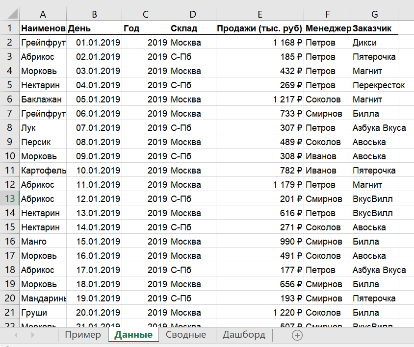
В примере выше атрибуты — это «Наименование», «День», «Год», «Склад», «Продажи (тыс. руб)», «Менеджер», «Заказчик». Они вынесены в заголовок таблицы.
Эта таблица послужит основой для построения нашего дашборда по продажам.
Если известно, для чего и для кого предназначен дашборд, легче понять, какие показатели должны выводиться на экран. Это могут быть любые количественные показатели, важные для организации: прибыль, продажи, численность сотрудников, количество заявок, фонд оплаты труда.
Также необходимо определиться с макетом — структурой — дашборда. Для начала достаточно будет прикинуть её на листе формата А4.
Пример универсальной структуры, которая подойдёт под любые задачи:
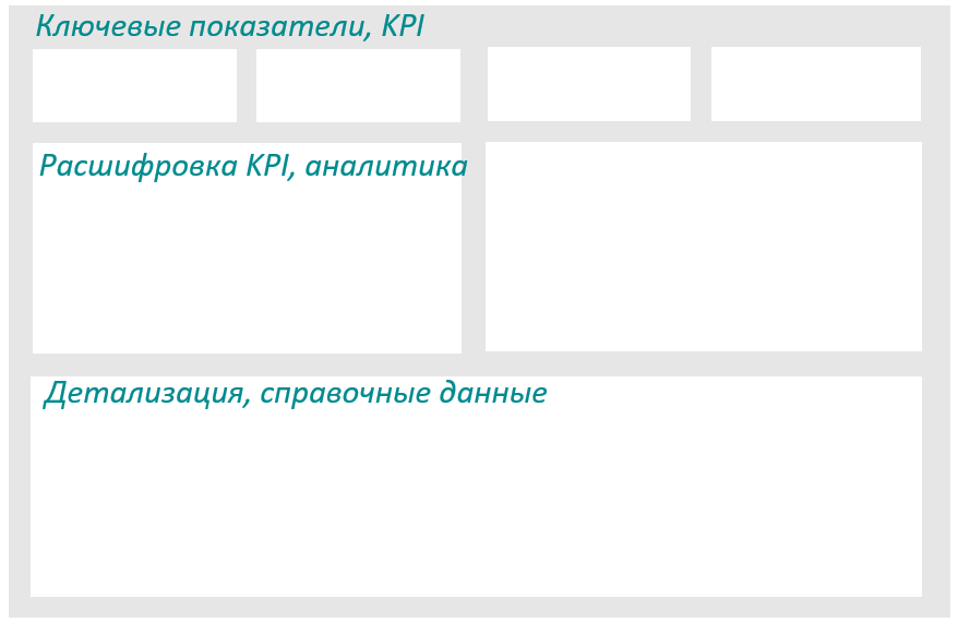
Количество информационных блоков может быть разным: это зависит от того, сколько метрик надо отразить на дашборде. Главное — соблюдать выравнивание по сетке.
Порядок и симметрия в расположении информационных блоков помогают восприятию и внушают больше доверия.
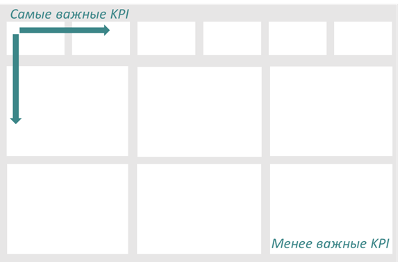
Помимо симметрии важно учитывать и логику расположения информационных блоков. Это связано с нашим восприятием: мы привыкли читать слева направо, поэтому наиболее важные метрики необходимо располагать слева направо и сверху и вниз, менее важные ― справа внизу:
— на основе таблицы с данными, приведённой выше в качестве примера плоской таблицы.
Таблицы будут показывать продажи по месяцам, по товарам и по складу.
Должно получиться вот так:
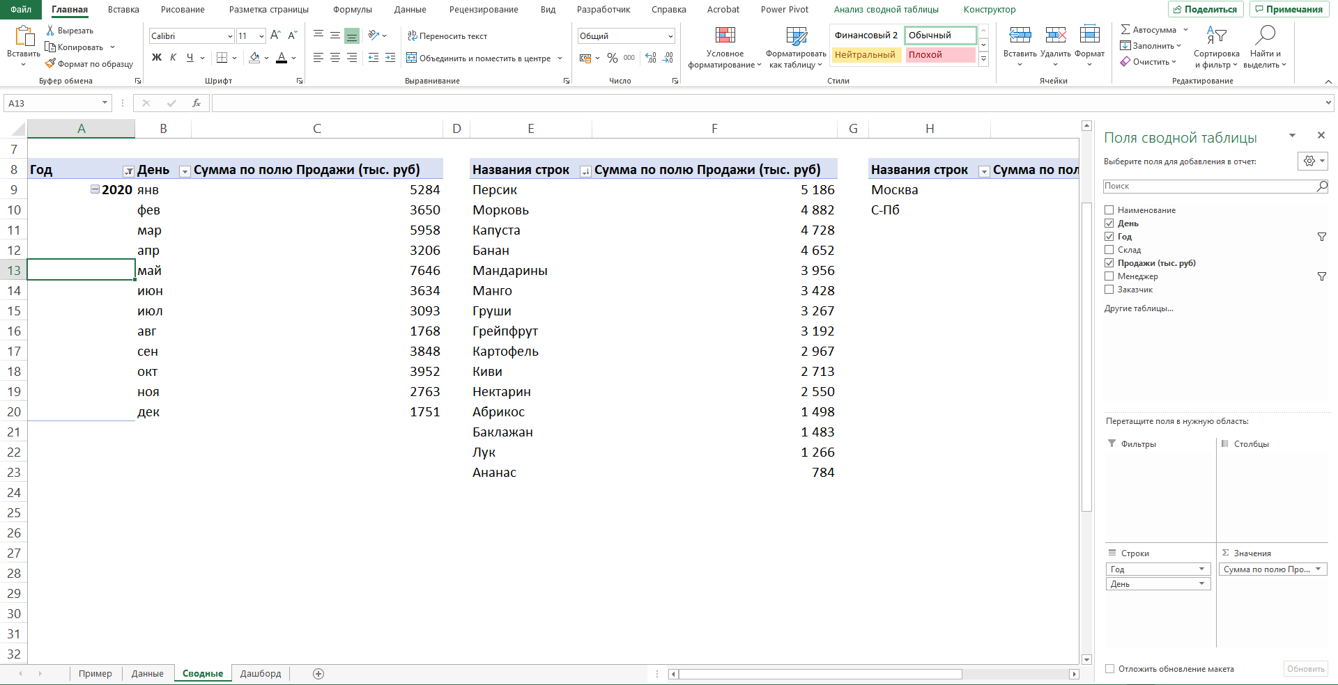
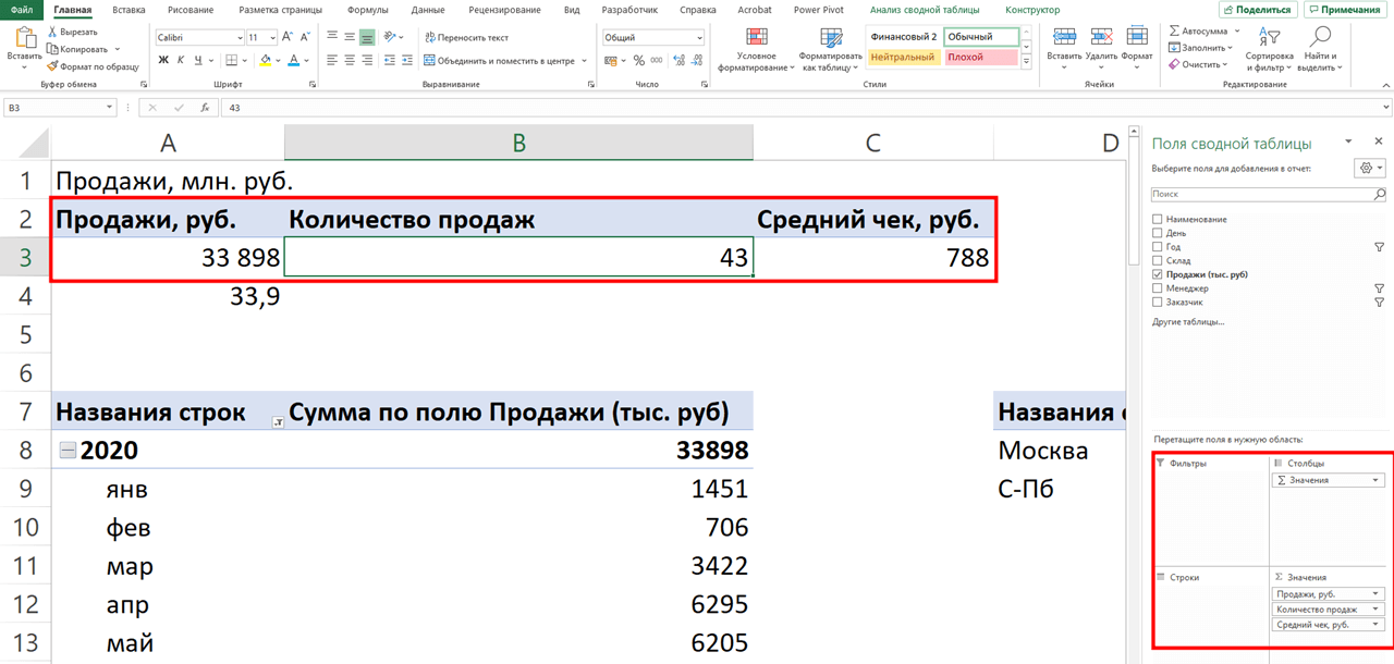
Также построим таблицу для ключевых показателей «Продажи», «Средний чек», «Количество продаж»:
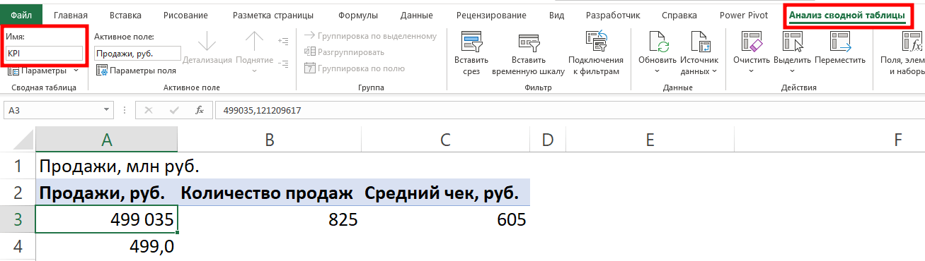
Чтобы в дальнейшем было проще ориентироваться при подключении срезов, присвоим сводным таблицам понятное имя. Для этого перейдём на ленте в раздел Анализ сводной таблицы → Сводные таблицы → в поле Имя укажем название таблицы.
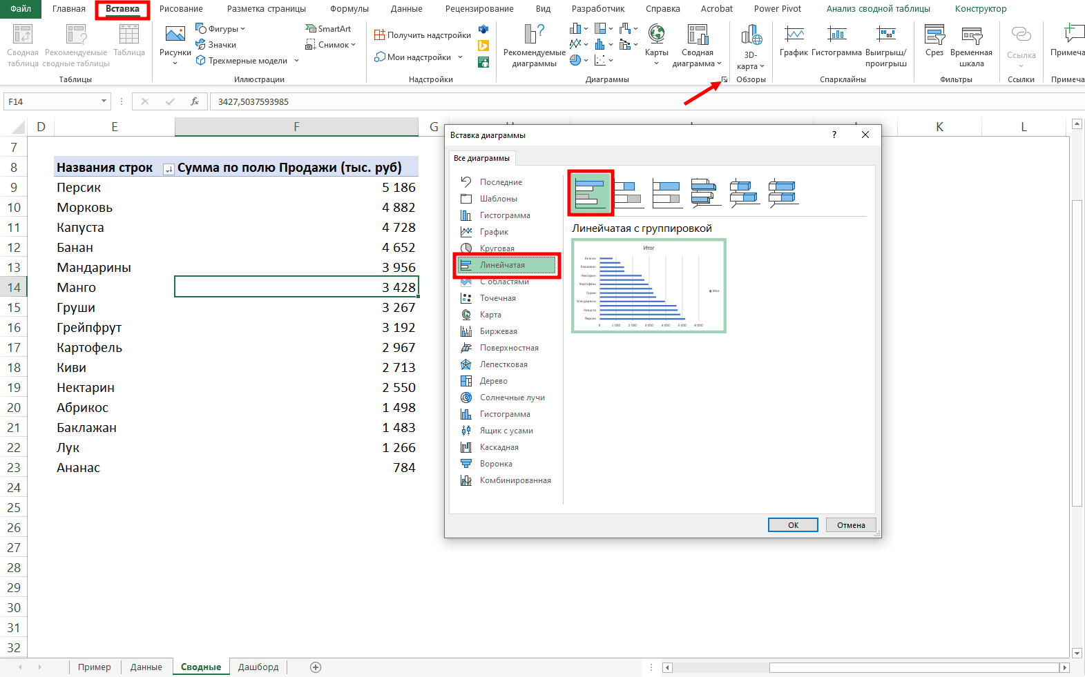
В нашем дашборде будем использовать три типа диаграмм:
- график с маркерами для отражения динамики продаж;
- линейчатую диаграмму для отражения структуры продаж по товарам;
- кольцевую — для отражения структуры продаж по складам.
Выделим диапазон таблицы, перейдём на ленте в раздел Вставка → Диаграммы → Вставка диаграммы → Выберем нужный тип диаграммы → ОК:
Отредактируем диаграммы: добавим названия и подписи данных, скроем кнопки полей, изменим цвет диаграмм, уменьшим боковой зазор, уберём лишние элементы — линии сетки, легенду, нули после запятой у подписей данных. Поменяем порядок категорий на линейчатой диаграмме.
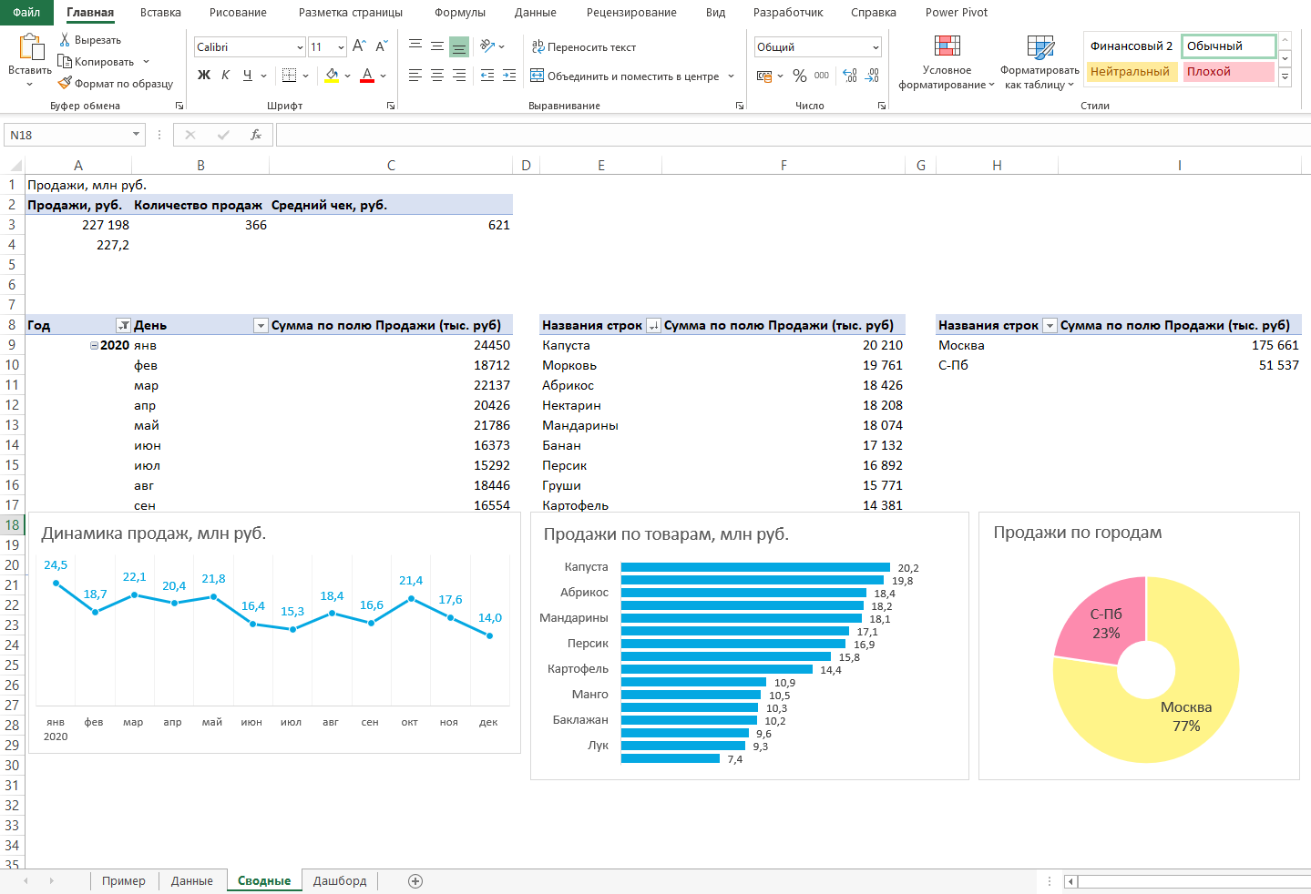
… и распределим их согласно выбранному на втором шаге макету:
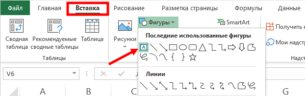
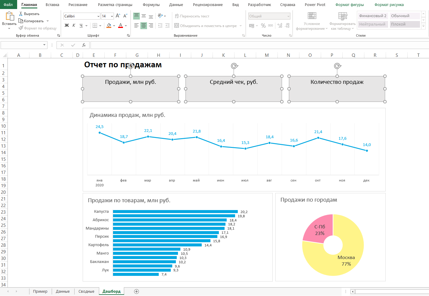
После размещения диаграмм необходимо вставить поля с ключевыми показателями: перейдём на ленте в раздел Вставка ⟶ Фигуры и вставим 3 текстбокса:
Далее сделаем заливку и подпишем каждый блок:
Значения ключевых показателей из сводных таблиц вставим также через текстбоксы — разместим их посередине текстбоксов с названиями KPI. Но прежде в нашем примере сократим значение «Продажи» до миллионов при помощи такого приёма: в сводной таблице рядом с ячейкой со значением поставим формулу с делением этого значения
на 1 000:
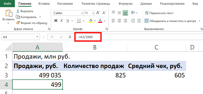
… и сошлёмся уже на эту ячейку:

То же самое проделаем с другими значениями: выделим текстбокс и сошлёмся через поле «Вставить функцию» на короткое значение в сводной таблице:
- Попробуете себя в роли аналитика в крупной ритейл-компании и поможете принять взвешенные решения об открытии новых точек продаж
- Научитесь основам работы с инструментами визуализации данных и решите 4 реальных задачи бизнеса
- 4 задачи — 4 инструмента: DataLens, Excel, Power BI,
Tableau
Срез ― это графический элемент в виде кнопки для представления интерактивного фильтра таблиц и диаграмм. При нажатии на эти кнопки дашборд будет перестраиваться в зависимости от выбранного фильтра.
Эта функция доступна в версиях Excel после 2010 года. Если нет возможности сделать срезы, можно воспользоваться выпадающим списком.
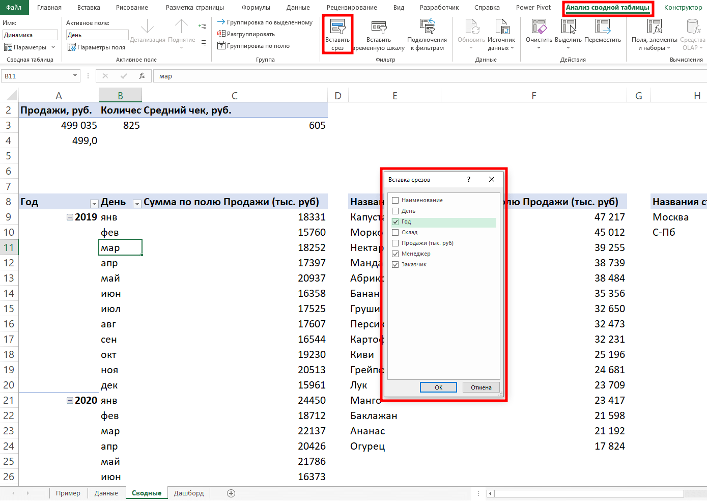
Для создания срезов выделяем любую ячейку сводной таблицы, переходим на ленте в раздел Анализ сводной таблицы ⟶ Вставить срез ⟶ поставим галочки в поля «Год», «Менеджер», «Заказчик», чтобы в дальнейшем можно было фильтровать данные по этим категориям.
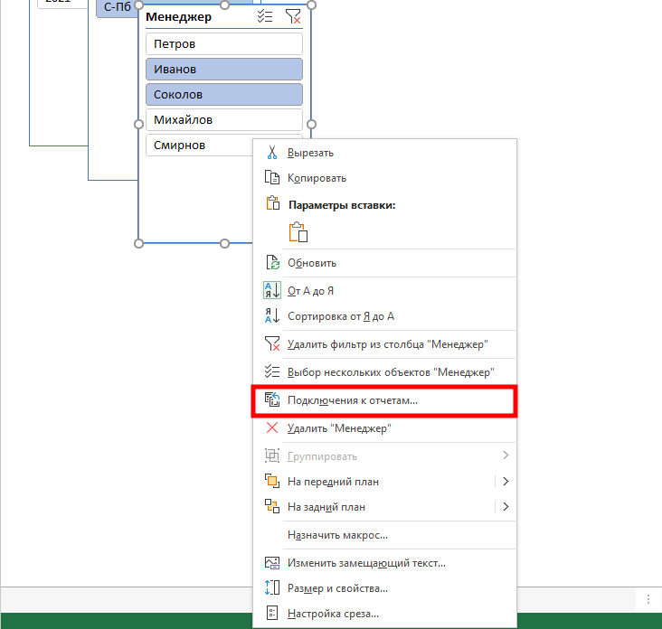
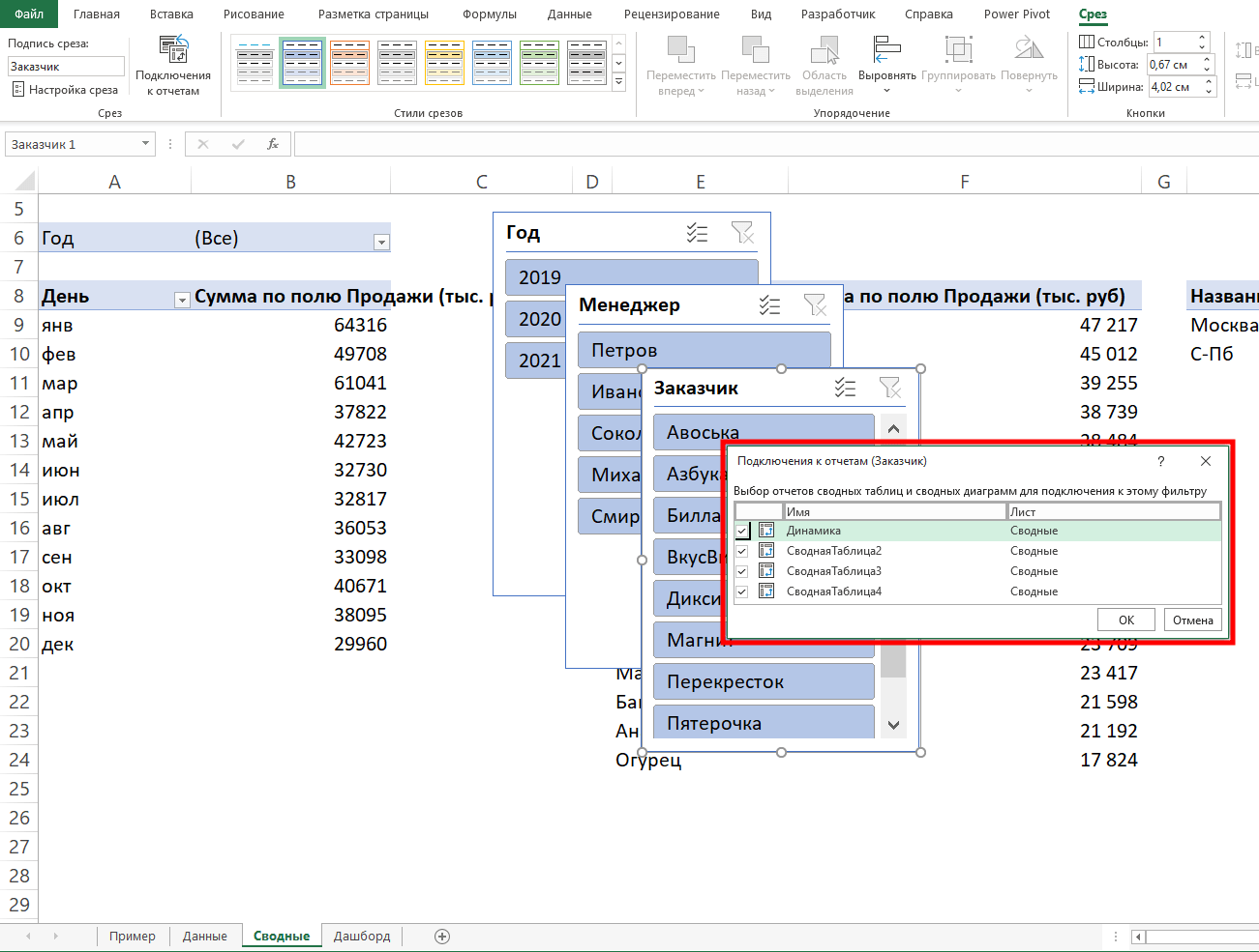
Если срез не работает и при нажатии на кнопки фильтра данные не меняются, подключаем его к нужным сводным таблицам: выделяем срез, кликаем правой кнопкой мыши, выбираем в меню Подключение к отчётам и ставим галочки на требуемых таблицах.
Повторяем эти действия с каждым срезом.
— и располагаем их слева согласно выбранной структуре.
Дашборд готов. Осталось оформить его в едином стиле, подобрать цветовую палитру в корпоративных цветах, выровнять блоки по сетке — и показать коллегам, как пользоваться.
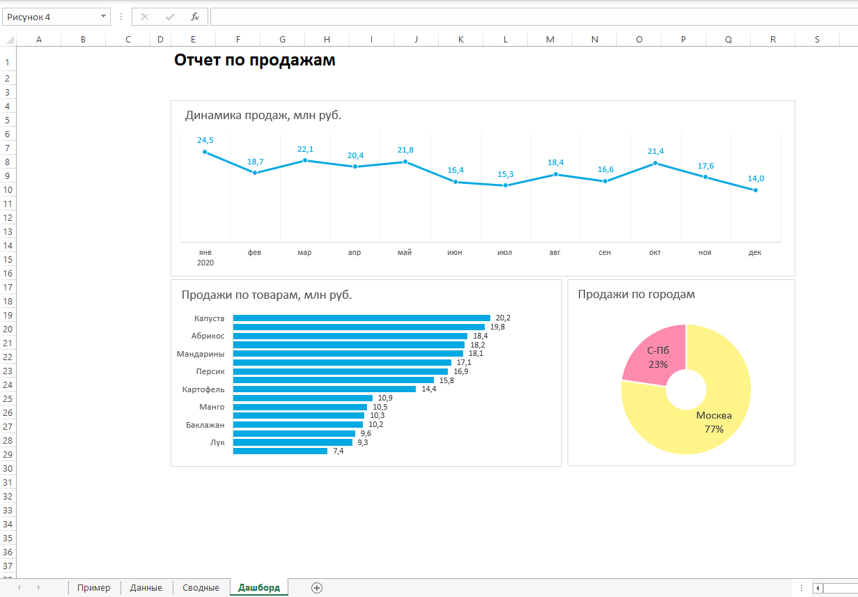
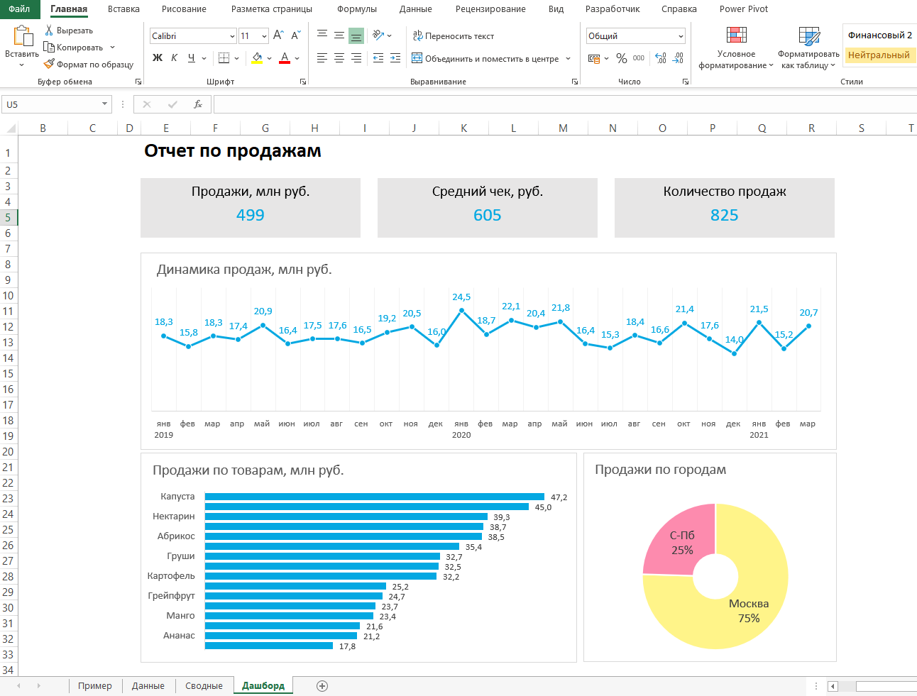
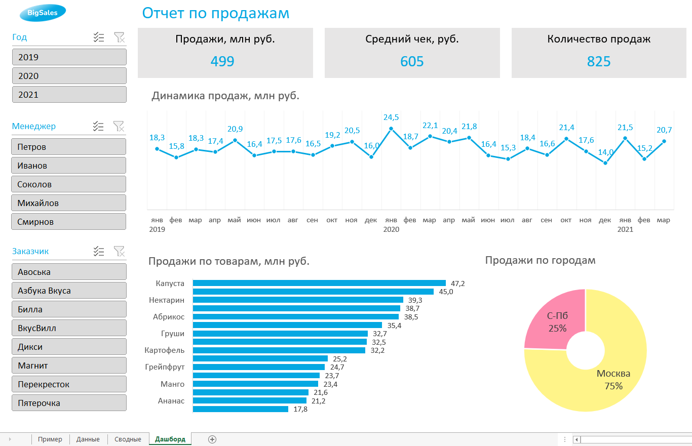
Итак, вот так выглядит наш дашборд для руководителя отдела продаж:
Мы построили самый простой дашборд. Если углубиться в эту тему, то можно использовать сложные диаграммы, настраивать пользовательские форматы срезов, экспериментировать с макетом, вставлять картинки и логотип.
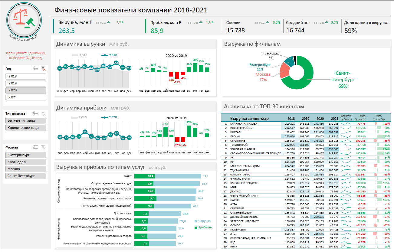
Немного практики — и дашборд может выглядеть так:
Не стоит бояться неизвестного — нужно просто начать делать, чтобы понять, что сложные вещи на самом деле не такие и сложные.
Принцип «от простого к сложному» — самый верный. Когда строят интерактивный дашборд впервые, многие испытывают искреннее восхищение. При нажатии на срезы дашборд перестраивается — очень похоже на магию. Желаем тоже испытать эти ощущения!
Мнение автора и редакции может не совпадать. Хотите написать колонку для Нетологии? Читайте наши условия публикации. Чтобы быть в курсе всех новостей и читать новые статьи, присоединяйтесь к Телеграм-каналу Нетологии.
Any organization primarily measures its growth in terms of Sales. An increment in Sales can be attributed to more customers, revenue, and more profits. Earlier the Sales data was tracked and analyzed manually but now analyzing Sales has become more complex due to huge amounts of varying and dynamic data. Organizations are looking for real-time Sales information and mechanisms to decrease their Sales analysis time.
Sales can help an organization identify the best & worst-performing assets and help them make better business decisions that will drive future Sales even higher. A Sales Dashboard Excel enables organizations to visualize their real-time Sales data and boost productivity. In this article, you will learn about the various key Sales metrics you should keep in mind while creating your Sales Dashboard depending on your use-case while setting up a Sales Dashboard Excel.
Table of Contents
- Understanding Dashboards
- Understanding Sales Dashboard
- Understanding KPI’s
- Understanding Key Sales Metrics for Your Sales Dashboard Excel
- Sales Growth
- Sales Target
- Customer Acquisition Cost
- Average Revenue Per Unit
- Customer Lifetime Value
- Customer Churn Rate
- Lead Conversion Ratio
- Sales Cycle Length
- Upsell Rate
- Cross-Sell Rate
- Steps to Set Up A Sales Dashboard Excel
- Step 1: Load your Data Into Excel
- Step 2: Set up your Sales Dashboard Excel File
- Step 3: Create a Table with Raw Data
- Step 4: Figure out Metrics and Visualizations
- Step 5: Build a Sales Dashboard Excel
- Step 6: Customize the Sales Dashboard Excel
- Adding Color to Elements
- Adding Color to Background
- Adding Title to Charts and Dashboard
- Step 7: Adding Animation
- Slicers
- Drop-down list
- Marcos
- Conclusion
Understanding Dashboards
A Dashboard is a very useful tool that brings together all the data in the form of charts, graphs, histograms, statistics, and many more visualizations which lead to data-driven decision-making. Dashboards contain actionable data. By looking at this data an organization can make key business decisions on the go.
Many tools help organizations build their Dashboards. For example tools like Power BI, Tableau, Excel help organizations build Dashboards suiting to their needs. Depending on the outcome you need, you can build Dashboards for Sales, Marketing, Engineering, and many more departments to track the performance. In this article, we will focus on the Sales Dashboard Excel.
Understanding Sales Dashboards
A Sales Dashboard is a visual representation of your organization’s data. You need to put a lot of thought into making a Sales Dashboard as it will affect all your future decisions. Sales Dashboards are used by executives, managers, or any employee in an organization and they should be designed in such a way that different employees can make use of them.
Before building a Sales Dashboard ask yourself the following questions:
- Why do you need the Dashboard and what kind of outcome are you looking for?
- Who are the employees that benefit from the Sales Dashboard?
- What key metrics are you going to visualize to get the best out of your Sales Dashboard?
- How are you going to integrate data into the Dashboard?
- How old is the Sales data in your Dashboard?
- What kind of template do you need to use for your Sales Dashboard?
Hevo, a No-code Data Pipeline helps to transfer your Sales data from Excel (among 100+ sources) to the Data Warehouse/Destination of your choice to visualize it in your desired BI tool. Hevo is fully-managed and completely automates the process of not only loading data from your desired source but also takes care of transforming it into an analysis-ready form without having to write a single line of code. Its fault-tolerant architecture ensures that the data is handled in a secure, consistent manner with zero data loss.
It provides a consistent & reliable solution to manage data in real-time and you always have analysis-ready data in your desired destination. It allows you to focus on key business needs and perform insightful analysis using a BI tool of your choice.
Get Started with Hevo for free
Check out Some of the Cool Features of Hevo:
- Completely Automated: The Hevo platform can be set up in just a few minutes and requires minimal maintenance.
- Real-Time Data Transfer: Hevo provides real-time data migration, so you can have analysis-ready data always.
- 100% Complete & Accurate Data Transfer: Hevo’s robust infrastructure ensures reliable data transfer with zero data loss.
- Scalable Infrastructure: Hevo has in-built integrations for 100+ sources that can help you scale your data infrastructure as required.
- 24/7 Live Support: The Hevo team is available round the clock to extend exceptional support to you through chat, email, and support calls.
- Schema Management: Hevo takes away the tedious task of schema management & automatically detects the schema of incoming data and maps it to the destination schema.
- Live Monitoring: Hevo allows you to monitor the data flow so you can check where your data is at a particular point in time.
Sign up here for a 14-day Free Trial!
Understanding KPI’s
KPI stands for Key Performance Indicators. These are very essential in order to create an efficient and useful Sales Dashboard Excel. KPI’s measure your progress toward a certain goal in a certain amount of time. Let’s assume that your goal is to achieve 100 leads in one month but you end up achieving 56 leads so now you may define a lead attainment KPI as achieved leads/ goal leads(56/100). This way you can define your own KPI’s.
Once you visualize your KPI if it is not satisfactory then you can try identifying the factors that lead to a low KPI and you can make the changes accordingly. Further, you will get to know the most commonly used KPI’s used for creating a Sales Dashboard Excel.
Understanding Key Sales Metrics for your Sales Dashboard Excel
Key Sales metrics also known as Sales KPI’s are very crucial to create the right kind of Sales Dashboard Excel that meets the needs of your organization. You can also define your own KPI’s to monitor your goals but for now, let’s talk about the 7 Sales KPI’s that are commonly monitored on the Sales Dashboard Excel:
- Sales Growth
- Sales Target
- Customer Acquisition Cost (CAC)
- Average Revenue Per Unit (ARPU)
- Customer Lifetime Value (LTV)
- Customer Churn Rate
- Lead Conversion Ratio
- Sales Cycle Length
- Upsell Rate
- Cross-Sell Rate
1. Sales Growth
This KPI measures the overall Sales growth. You have to fix a period of time (ex. 2 years, 5 years, etc) and calculate the percentage of change in Sales from the last Sales period to the current sales period. An increase in this indicates that your product is doing well and a decrease indicates that you need to look for issues that are leading to a decrease in sales.
2. Sales Target
This KPI measures the percentage of Sales Revenue against Target Revenue.
If the percentage is low you have to look further into which division/ asset is generating the least revenue and take measures to increase the revenue from these.
3. Customer Acquisition Cost (CAC)
Customer Acquisition Cost (CAC) is the total revenue spent by a company to convert them into customers. This includes money spent on marketing, personnel, discounts, and anything which has a role in acquiring the customer. This is an important measure because you should be able to recover this cost over a period of time when you convert them into customers. If you are unable to recover this amount then you have to cut back on expenditures in the acquisition.
4. Average Revenue Per Unit (ARPU)
This KPI is your organization’s average revenue. To calculate the Average Revenue Per Unit (ARPU) divide your whole revenue by the number of customers. It is basically the average revenue a customer brings to your organization. If ARPU is less than Customer Acquisition Cost (CAC) you may run into troubles and may face a loss so it is important to keep tracking this metric.
5. Customer Lifetime Value (LTV)
To calculate this KPI first calculate the Average Customer Lifetime (total lifetime of all the customers/ number of customers). Depending on this now calculate how much revenue can be generated during this average lifetime which is the Customer Lifetime Value(CLV). You can use this to set your CAC which is less than CLV to ensure profits.
6. Customer Churn Rate
A business can grow as long as it retains old customers and gains new ones. Customer Churn Rate gives the count of the customers that left your business over a period of time. It is important to maintain a low churn rate because a high churn rate ensures loss of revenue. So it is very important to retain existing customers.
7. Lead Conversion Ratio
Leads are potential customers of your organization. A person becomes a lead when he/she visits your website. So if you can track the leads and promote your product you will observe an increase in sales. Set up a target ratio and try to reach it and keep monitoring this ratio.
8. Sales Cycle Length
It is important to include your Sales Cycle length in your Sales Dashboard because keeping track of metrics from time to time is efficient. Initially, the whole process of converting the leads into customers takes a long time. Companies aim towards decreasing their Sales Cycle length. Also, as the company becomes more acclaimed, the conversion into customers becomes easy which reduces the Sales Cycle length.
9. Upsell Rate
Upsell rate talks about the number of customers that purchased a product or accessory related to their previous purchase. A good Upsell rate implies that your products are satisfactory to your customer and he/she is inclined to purchase related to your company.
10. Cross-Sell Rate
Cross-sell rate is similar to Upsell Rate. The only difference is that you pitch different products from their previous purchase to your customers and this rate tells you how many people are willing to buy other products. A good Cross-sell rate is an indicator that all the products in your company are being loved by your customers. Make sure to include both Upsell and Cross-sell Rates in your Sales Dashboard Excel.
After you identify all the KPI’s and understand what you want to do with your Dashboard follow the below-given steps to create a Sales Dashboard Excel:
- Step 1: Load your Data Into Excel
- Step 2: Set up your Sales Dashboard Excel File
- Step 3: Create a Table With Raw Data
- Step 4: Figure out Metrics and Visualizations
- Step 5: Build a Sales Dashboard Excel
- Step 6: Customize the Sales Dashboard Excel
- Step 7: Adding Animation
Step 1: Load your Data Into Excel
Since you are creating a Sales Dashboard in Excel you must load your data into Excel first. There are ETL tools that can help you achieve this. ETL (Extract Transform Load) extracts data from a source and loads them into a destination. There are also some ODBC connectors that help move your data from your apps to Excel. Read about moving your data into Excel using ODBC connectors here.
Step 2: Set up your Sales Dashboard Excel File
Once your data is available in Excel open a new Excel Workbook & create two tabs/ sheets. One is Sales Dashboard and the other is for Raw Data (here you can hide your raw data). Look at the image below to understand.
Step 3: Create a Table with Raw Data
The Raw Data tab is where you load your data using an ETL tool. Make sure that there is only one item in each cell. Also, for numerical columns in the table, you can add all the items present in the column by clicking on the empty cell at the end of the column and type the =SUM formula.
Now drag your mouse from the first item of your cell to the last item. Now type a closed bracket. This will look some like:
Step 4: Figure out Metrics and Visualizations
Once you figure out the metrics you can use Excel tools to create visualizations for those metrics. These visualizations include pivot tables, auto shapes, charts, names ranges, Marcos, etc. All these visualizations are very simple to make and an Excel Dashboard can easily be set up.
Step 5: Build a Sales Dashboard Excel
Go to your Sales Dashboard Excel sheet. In the Dashboard sheet, select Insert from the top left corner of the window. Now you will be able to see a lot of different kinds of charts offered by Excel. Choose the chart of your choice. Now the chart will appear on the screen. Right-click with your mouse on the chart and add the data sources, names and labels. After making the changes click on the Ok button.
Step 6: Customize the Sales Dashboard Excel
Now you can customize your Sales Dashboard Excel and make it look attractive by adding colours and changing the fonts. The more attractive it is, the more you will want to work with your Dashboard. You will learn about:
- Adding Color to Elements
- Adding Color to Background
- Adding Title to Charts and Dashboard
1. Adding Color to Elements
To customize your Sales Dashboard Excel click on the element of the chart that you want to add colour to. Now go to the Home tab and select Font where you can find a paint bucket symbol. Click on it and change the colour. Also in the Font option, you can change the font if it is a text element.
2. Adding Color to Background
To fill the background of a chart with colour, use your mouse to right-click on the chart and select Format Chart. In the list that appears choose Fill. Now choose Solid Fill. Go to the Font section and you can see a bucket. Click on the bucket and choose a background colour of your choice.
3. Adding Title to Charts and Dashboard
To add your chart title, click on a chart title (this is a random name already created by default by Excel) and click on Font group. Now you can select your font type, size, and colour of your title.
To add a title to your Sales Dashboard Excel, put your cursor in the upper-right cell and right-click on it, and select Insert and click on Entire Row. Do this repeatedly until you have space to add a title. Then, select a couple of cells in the first empty row, and in the Alignment group, click Merge and Center. After all this, you’ll have enough space to add your Dashboard title.
Step 7: Adding Animations
Interactive Dashboards are fun to work with. Excel offers some interesting dynamic elements. Let’s talk about these elements:
- Slicers
- Drop-Down List
- Macros
1. Slicers
Slicers can be used to modify tables and pivot tables. Slicers have buttons that facilitate this feature. So they filter data and display what kind of data is being filtered. Read more about creating Slicers in the official documentation.
2. Drop-Down List
Drop-down lists are some of the common dynamic elements everybody knows about. It makes any page looks less bulky, neat and categorized. Drop-down lists are used to limit user inputs to acceptable ones. Read more about creating drop-down lists in the official documentation.
3. Macros
Codes have become popular because anyone doesn’t want to repeat a set of tasks again and again. Similarly if in your Sales Dashboard Excel you want to perform a task repeatedly you can do it by using Marcos. This feature records your set of actions and then performs them without your intervention. Read more about creating Marcos in the official documentation.
Conclusion
Keeping track of all your Sales metrics is essential for boosting Sales and identifying underlying problems. Every metric in your Sales Dashboard Excel will help you understand more about your company’s progress and it also allows you to make quick and accurate business decisions.
If you are looking for sample templates for Tableau Sales Dashboards you can find these here, and if you are planning to set up Sales Dashboards in Power BI you can find the guide here.
Integrating and analyzing your Sales data from a huge set of diverse sources can be challenging, this is where Hevo comes into the picture.
Visit our Website to Explore Hevo
Hevo is a No-code Data Pipeline and has awesome 100+ pre-built integrations that you can choose from. Hevo can help you integrate your sales data from numerous sources and load them into a destination to analyze real-time data with a BI tool and create your Dashboards. It will make your life easier and make data migration hassle-free. It is user-friendly, reliable, and secure.
Want to take Hevo for a spin? Sign Up for a 14-day free trial and experience the feature-rich Hevo suite first hand. You can also have a look at our unbeatable pricing that will help you choose the right plan for your business needs!
Share your experience of learning about Sales Dashboard Excel. Tell us in the comments below!
For example, consider how to make a dashboard in Excel to visualize sales funnel conversion data with interactive capabilities and dynamically changing information on charts and graphs.
An example of building a sales funnel conversion dashboard in Excel
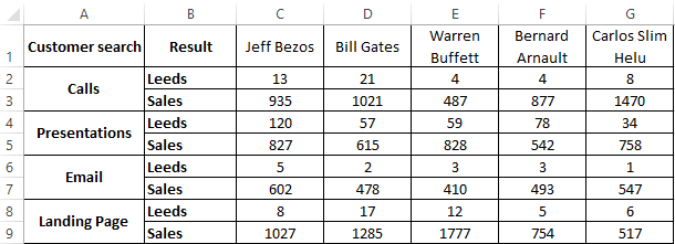
For example, simulate a situation. From the CRM system, 2 reports were exported in the Excel table format (in two tables) for subsequent visual analysis of the conversion and effectiveness of the sales funnel of the top 5 managers:
- Jeff Bezos.
- Bill Gates.
- Warren Buffett.
- Bernard Arnault.
- Carlos Slim Helu.
Looking ahead, it is worth paying attention to the fact that both reports are presented in tables with combined cells. Therefore, during their data processing, the OFFSET function will be used for sequential sampling of indicator values from tables through one row with even and odd numbers:
- The first report displays detailed information about the first stage of the Sales Search customer funnel. This report expresses the effectiveness in the results of the work of sales managers, therefore, indicators of the ratio of the number of leads (orders) to the amounts of closed transactions — sales are taken. All values of the Leads and Average Check indicators are segmented not only by managers, but also separately by source for searching and attracting customers:
- The second report is located in the table on the same sheet called “Data”. It provides general information on going through all stages of a sales funnel. Thanks to the dates, we can calculate how many days it took for each stage of the funnel starting from the start date of the advertising campaign project. But thanks to the visualization of data on the dashboard, we can clearly see this indicator and analyze it more efficiently and comfortably in order to draw the right conclusions for quickly making the right decision. Relative bounce rates are also presented here, which is important when analyzing the sales funnel conversion in Excel:
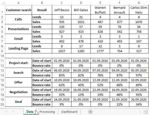
This report is very important in analyzing the sales funnel conversion, although not all analysts take it into account and this is sad.
Source data processing for visualization of indicators in charts
On the second sheet “Processing” of the dashboard are formulas with calculations. All names of indicators are taken from the first sheet “Data” using the links:
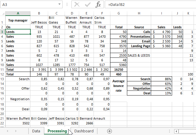
Thanks to spring links in processing the source data of the first sheet, you can use this dashboard as a template. It is enough to just change the names with the indicators in the source data, and the template will automatically update all the values on the main Dashboard sheet.
Next, we proceed directly to the analysis of the device of the dashboard itself and its visualization of the data initially presented in tabular form.
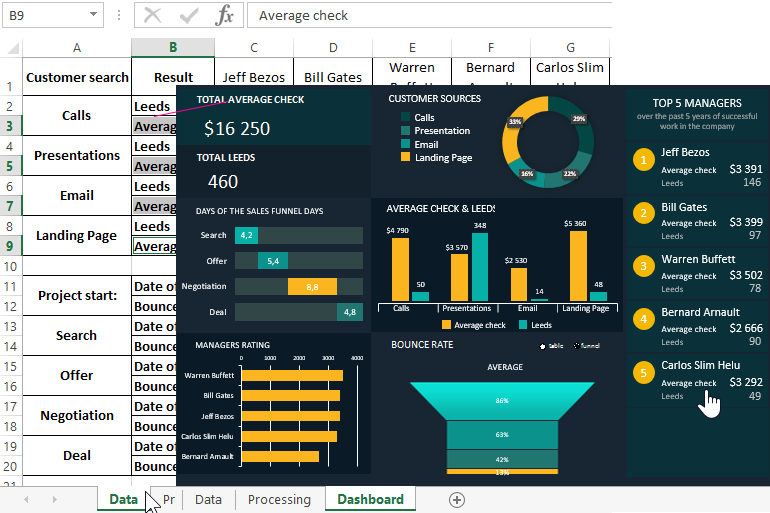
Creating a dashboard for analyzing customer conversions in leads and sales
Dashboard for analysis of sales funnel conversion by managers, consists of 7 + 1 blocks. Why learn +1 at the end of the visualization description. The dashboard has not only dynamic charts and graphs, but also interactive features. Thanks to them, we can individually exclude managers from the report in order to analyze how much the overall picture will change. Or see the same indicators for each manager individually to compare with the overall results of the work performed:
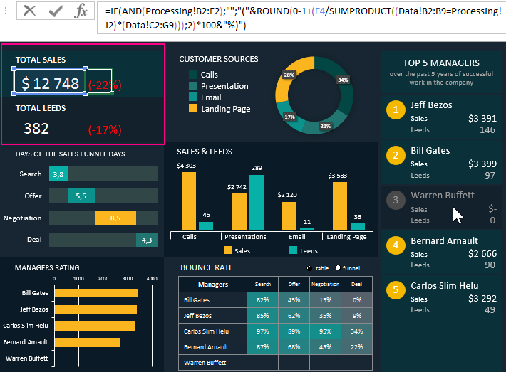
The first block in the upper left corner displays the total total sales figures and the total number of leads of all active managers (in this case, 4 as shown in the figure above). When one of the 5 managers is disabled, relative percentages are displayed next to the total absolute indicators of the report. They inform us of how much the total amount of sales or leads decreased as a percentage, after exclusion of one of the managers from the advertising company.
As can be seen from the formula indicated in the figure above, to calculate this indicator, the arguments are referenced by external links to both sheets:“Data” and “Processing”.
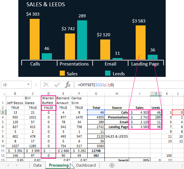
Analysis of the profitability of sources of customer acquisition in Excel
The second block, from the top to the middle, shows in the ring diagram what percentage of sales in money is each source of customer acquisition:
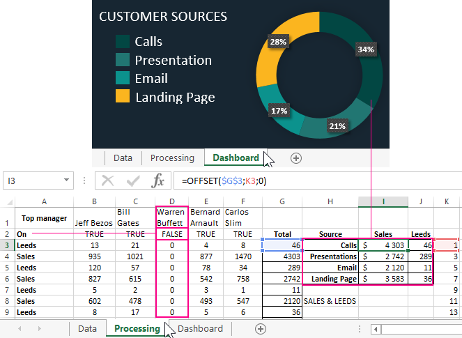
The data calculation formulas for this diagram are on the Processing sheet in the cell range H3:I6. According to this visualization, we immediately focus not only on which segment turned out to be the most profitable, but also how significant differences are in relation to other segments.
Also note that the third manager, Warren Buffett, now contains only zero values in the table, since it was turned off on the dashboard. This is indicated by the FALSE value in cell D3 in the row with the heading “Enabled”. This is the principle of the functioning of the dashboard interactivity when the user switches the buttons on the main sheet. And after that, the whole picture of the report plays from this table, because most of the formulas are linked by links. This is the right approach when creating a report template.
For aesthetics, the legend was built from figures and inscriptions with links to the corresponding names of the sources. External links in the inscriptions also contribute to the ability to use the dashboard as a template. It is enough to change the name of the source only on the “Data” sheet, and it will automatically change on all the corresponding signatures of the indicators of charts and dashboards.
Analysis of conversion dates at each stage of a sales funnel in Excel
The next block 3 “Stages of the sales funnel in days” shows how many days it took on average for each stage:
- Search for customers.
- Presentation of the proposal.
- Negotiating before concluding a deal.
- Closing a transaction is a fact of sale.
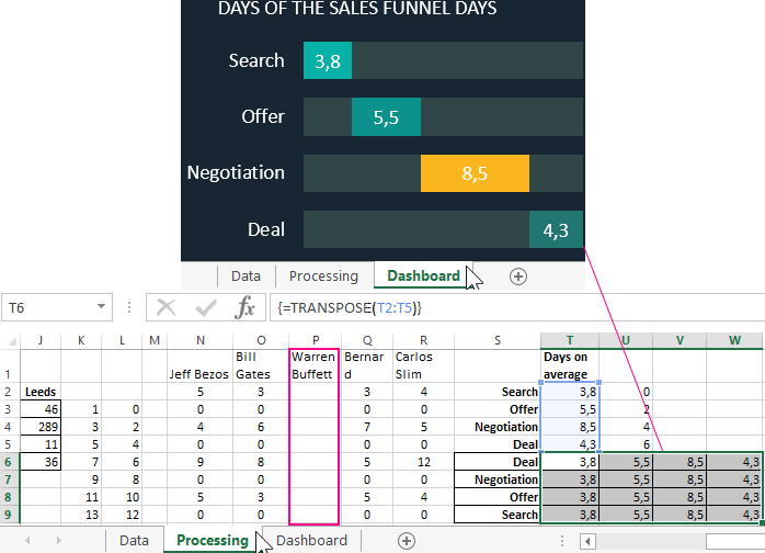
To construct this visualization, we used a normalized bar histogram with accumulation based on values from the T6:W9 range as shown in the figure above. Also note that the «Warren Buffett» column is empty in the cell range P2:P9. In this table N1:R9 are intermediate formulas for selecting the necessary values from the «Data» sheet. Further, in the range of cells T2:T5, using the OFFSET function, values are collected in one column selected through one row (with paired numbers). And after the range T2:T5 is transposed by the array function {CTRL + SHIFT + Enter} TRANSPOS to the range T6:W9, to build a normalized ruled histogram with accumulation.
Conversion of the number of leads to sales by managers
The 4th block in the «Sales and Leads» center displays the sales levels and the number of leads on different axes of the vertical Y axes. All levels are presented in pairs for each source of customer acquisition. Thus, we can analyze the relationship between the growth in the number of leads and the size of sales. It was possible to draw up such a schedule by superimposing two histograms with a grouping. On the top layer is a graph with a transparent background. Axis signatures and legend design are also built from figures and inscriptions for a more aesthetic look:
Values for graphics visualization are taken from the ranges I3:I6 and J3:J6 on the “Processing” sheet.
Dynamic chart of sales managers ranking
In the lower right corner is the 5th block “Rating of managers”. This is an ordinary bar chart with a grouping showing sales volumes for each manager. Its only feature is that it constantly sorts the signatures of the X axis and its indicators in descending order due to the use of the BIGGEST function in the source of its data on the “Processing” sheet:
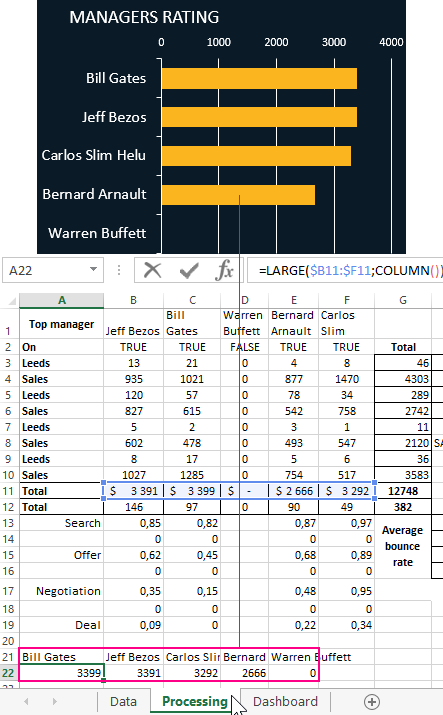
The data range for the bar graph is A21:E22. Two lines of this range are filled with two different formulas. Formulas should be considered first from the second line of this range of cells:
- The second line contains the formula from the combination of the LARGEST and COLUMN functions, which allow you to sort the value of the final row of the first table on this sheet in the range B11:F11:
- The first line contains a formula from a combination of the INDEX and SEARCH functions to select the names of managers from the first table according to the values of the second row of this range. Thus, the order of filling the cells of the first row with the names and surnames of managers is filled in accordance with the sorting in descending order of their sales volumes:
As a result, we get a histogram for dynamic visualization of ratings of sales managers, which changes the order of the displayed series in accordance with other changes in the report.
Bounce rate at all levels of the sales funnel for conversion analysis
Below the middle is the 6th block “Percentage of failures”. It is a smart table with a heatmap created using conditional cell formatting in Excel:
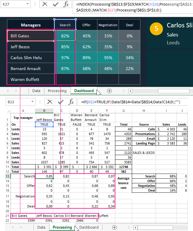
First, using the formula from external links and functions of the TRASP array, the row headers in the «Managers» column are filled with values from the cell range A21:E21 of the «Processing» sheet.
And then, on the basis of this data, all necessary values are selected from the range B13:F19 to fill in the tabular part.
Dynamic Sales Funnel in Excel
An important point! On this block there is a switch (Option Button) “Table / Funnel”. With it, we can activate and enable the hidden +1 block “Average indicator”. As a result, instead of the table of the sixth block, a sales funnel diagram will be displayed with averaged share size values at each funnel stage:
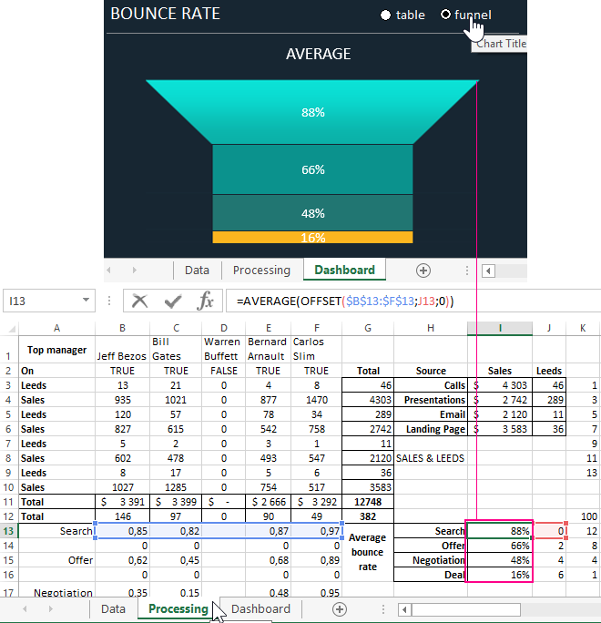
A sales funnel diagram is built from a combination of a normalized histogram with accumulation and figures drawn and combined in MS PowerPoint:

Just for each row of the histogram, you should copy the corresponding figure and paste it directly into the CTRL + V row. The figures are attached on the sheet «Processing» in the Excel file with an example of the template for this dashboard, which can be downloaded from the link at the end of the article.
To operate the switch and hide the sales funnel diagram, the following macro code is used:
Sub Voronka()
Dim list As Worksheet
Dim opt1 As Shape
Dim charvoronka As ChartObjectsSet list = Sheets(«Dashboard»)
Set manag1 = list.Shapes(«Option Button 8»)If manag1.OLEFormat.Object.Value = 1 = True Then
list.ChartObjects(«Diagram 32»).Visible = msoFalse
Else
list.ChartObjects(«Diagram 32»).Visible = msoTrue
End If
End Sub
To add the switch itself, select the tool:“DEVELOPER” — “Controls” — “Paste” — “Switch”.
Interactive dashboard and chart management buttons
And finally, the seventh block of the “Top 5 Managers” is a dashboard control panel of 5 buttons:
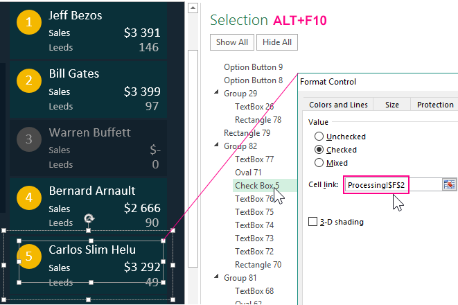
The buttons are composed of figures and inscriptions with external links to the corresponding values of the cells of the sheet «Processing». In addition to the figures, the design contains hidden (with a transparent background) controls «Check Box» (Check Box). Each element is assigned a macro code, which, when pressed, changes the font color of labels and shape fills. In addition, the properties of the flag settings indicate the connection with the cell of the first table on the «Processing» sheet where the flag sends the key value TRUE or FALSE.
The result is a stylish, functional and useful dashboard — a tool for visualizing important data that dynamically changes when interacting with a user:
 Free Download sales funnel conversion dashboard in Excel
This dashboard can be used as a template for your indicators. But not only indicators, but also names of names can be changed on the first sheet “Data” and as a result they will be changed on all other sheets.
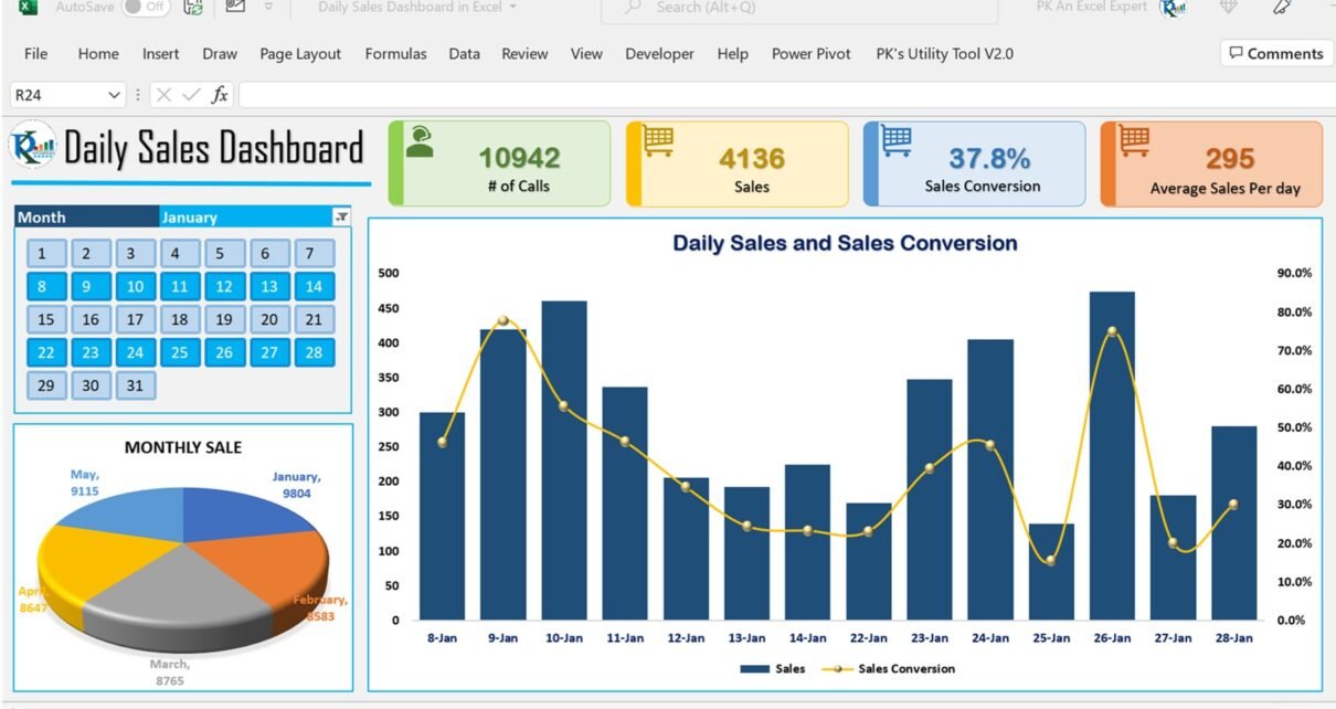
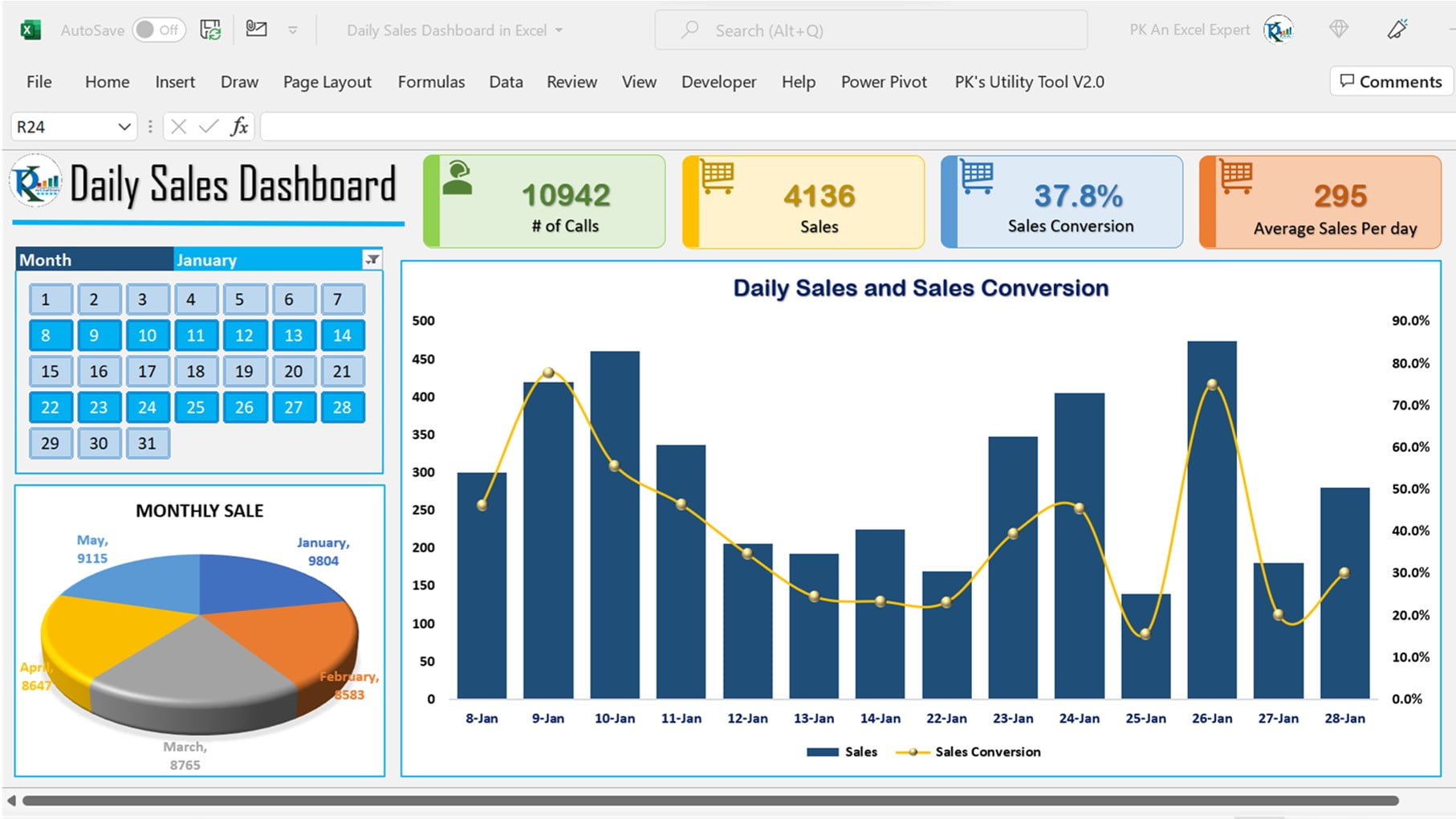
In this article, we have created a Daily Sales Dashboard to analyze the Daily Sales trends. We have displayed 4 metrics in this dashboard-
# Of Calls:
The number of calls made by telecallers to generate the sale.
Sales:
Number of Sales made by telecallers.
Sales Conversion:
Sales conversion is the ratio of Sales and Calls.
Average Sales Per Day:
Average sales made by telecallers in a day.
Download our free dashboards-
- Annual Sales Calendar for Sales Dashboard in Excel
- Comparative Analysis Dashboard in Excel
- KPI Dashboard with Tooltip in Excel
- Dynamic Dashboard with Tablet and Mobile shape in Excel
- Performance Dashboard
- Top/Bottom Analysis dashboard in Excel
- Fully Automated Excel dashboard with multiple source files
- C-SAT Dashboard
- Outbound Dashboard in Excel
Watch the step-by-step video tutorial:
Click here to download the template file.

Meet PK, the founder of PK-AnExcelExpert.com! With over 15 years of experience in Data Visualization, Excel Automation, and dashboard creation. PK is a Microsoft Certified Professional who has a passion for all things in Excel. PK loves to explore new and innovative ways to use Excel and is always eager to share his knowledge with others. With an eye for detail and a commitment to excellence, PK has become a go-to expert in the world of Excel. Whether you’re looking to create stunning visualizations or streamline your workflow with automation, PK has the skills and expertise to help you succeed. Join the many satisfied clients who have benefited from PK’s services and see how he can take your Excel skills to the next level!
Sales Dashboard in Excel is the new PB&J.
In addition to helping you keep track of sales information (which is especially handy if you’re managing multiple teams), some sales dashboards can also help you engage your reps and exceed quota right after it’s been set.
In this post, I’m going to show you how to create a sales dashboard in Excel, Spinify, and Salesforce.
It’s time to rock the socks off your sales process!
How to Create a Sales Dashboard in Excel
Here’s the thing: we may joke about Excel, but it’s still incredibly effective if you work with numbers.
(And, as we all know, sales teams live and breathe their numbers.)
So how do you set up a simple yet powerful sales dashboard in Microsoft Excel?
Step 1. Lay the Groundwork
Before you power up Excel, make sure you know what you want to track with your sales dashboard.
Identify KPIs (key performance indicators) that will be meaningful to you and your sales teams, and then decide on data types and sources you’ll track.
Make sure you understand:
- Where your data will come from (Sources, and will you manually import it or sync Excel with a different tool?)
- Who the dashboard is for (Is it for you as the sales manager, for sales reps, top management, etc.)
- How often the dashboard has to be updated
Step 2. Import Your Data
Now, you can either manually import the data by copy/pasting, or you can use an integration that syncs Excel to your other apps.
Many sales teams use ODBC data sources for that, as they can be refreshed every time you need to pull up new data.
To do it, navigate to Get Data > From Other Sources > From ODBC.
Step 3. Set Up Your Excel Dashboard
It’s a good idea to create at least two tabs in your workbook AKA sales dashboard.
This way, the first tab can be your dashboard where you’ll see all the results at a glance (cells will reference to cells in the second tab).
You can enter raw data in the second tab.
Step 4. Advanced Functions and Design
Finally, Excel has plenty of options for charts and formulas that may be useful to you.
You can use Gantt charts, create dropdown lists with VLOOKUP for interactivity, and much more.
You can even automate some of the data-related tasks with a Macro.
But if you’re looking for something leaner and more powerful, you can also…
Create a Sales Dashboard in Spinify
Here’s the thing: Excel works.
But it only works if you have enough patience to sift through data and don’t need visual stimuli to reduce time wasted on figuring out the numbers.
This is why visual sales dashboards like Spinify work like a charm!
Not only will you be able to track your KPIs, but you’ll also engage and motivate your sales reps at the same time.
Step 1. Choose a Pre-Set Spinify Sales Dashboard Template, Customize It, and Add Integrations
Unlike Excel, Spinify doesn’t make you create your sales dashboards from scratch.
You can use a pre-set sales dashboard and customize it to fit your:
- KPIs and metrics
- Workflow
- Company culture
Since Spinify supports a variety of integrations, you’ll be able to import your data with just a few clicks.
Step 2. Set Your Primary and Secondary KPIs
Spinify is actually a sales engagement dashboard.
You’ll be tracking your results and your reps’ performance at the same time.
For example, let’s say you care about the number of sales made (duh). You can set up your KPIs to reflect that in the Spinify sales dashboard.
However, you need to look further and understand which behaviors drive those results.
Let’s say that your team is at their most successful when they make enough phone calls. You can use that as your second KPI.
And then…
Step 3. Motivate Your Team
Spinify also comes with gamification features such as:
- Achievements, points, badges, and rewards
- Performance grids and scorecards
- Leaderboards that can be displayed on office TVs and on mobile devices
You can set up all of these in just a few steps and reward your sales reps for behaviors that drive progress.
Step 4. Success!
I don’t have to tell you that the best way to improve your results is to track them in the first place.
However, you may not know how successful gamification is at improving individual employee performance.
With Spinify’s sales dashboards, your employees will be:
- More productive
- More engaged
- Happier at work
And if that doesn’t sound like a sales success formula, I don’t know what does!
How to Create a Sales Dashboard in Salesforce
Finally, Salesforce is a great tool for creating purely functional sales dashboards.
You’ll be able to track everything that matters to you through it, and it sure beats Excel’s clunkiness.
Step 1. Create Your Dashboard and Import the Data
First, you need to prepare a report with the data you need to display, which you’ll then import in Salesforce.
Then, navigate to Dashboards tab > Go to Dashboards List > New Dashboards.
Step 2. Add the Components You Need
You can drag and drop sales dashboard components like charts, gauges, and tables directly into your dashboard.
Step 3. Filters and Refreshing
Finally, you can also set up filters to view the data in terms of performance metrics (e.g. Performance by products).
The data isn’t refreshed in real-time, so make sure you manually hit “Refresh” whenever you want the Salesforce dashboard to pull new results.
Choosing the Best Sales Dashboard Tool
The ideal sales dashboard depends on your volume and your needs.
However, Excel is pretty bare-bones. If you’re not managing more than 5 salespeople and 100 sales per month, you could get by.
Salesforce is a good fit if you’re running mid-sized teams that don’t need to be motivated.
But if you want to motivate your sales reps and drive results day in and day out, regardless of your volume, go with Spinify.
Not only is it a sales dashboard, but it’s a powerful sales gamification tool.
Coach, motivate and improve your team with just a few clicks.
Sign up for a free 14-day trial