Sales charts in excel - Word и Excel - помощь в работе с программами

Introduction

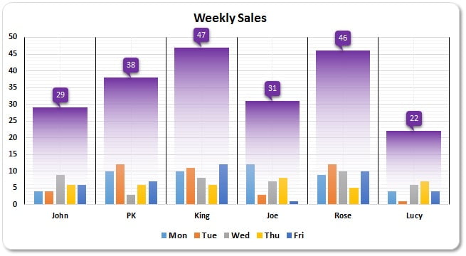
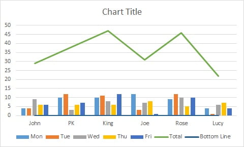
In today’s business world, charts and graphs have become an essential part of data analysis. They help to present complex data in a clear and concise manner, allowing us to quickly analyze and draw conclusions from the information presented. In this article, we will learn how to create a weekly sales chart in Excel. This chart will display employee-wise weekly sales and Mon to Fri sales trend of each employee in small columns. By the end of this article, you will have the knowledge to create an informative employee-wise weekly sales chart that will help you to better understand your business’s sales data.

Weekly Sales Chart

Data Set for Weekly Sales Chart

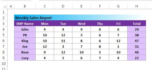
To create the weekly sales chart in Excel, we will first need a data set. Below is the data set that we will use for this example:

Data Set for Weekly Sales Chart

Steps to create Weekly Seles Chart in Excel-

Inserting the Chart

Add a support column “Bottom Line” as keep values as Zero

Bottom line support column

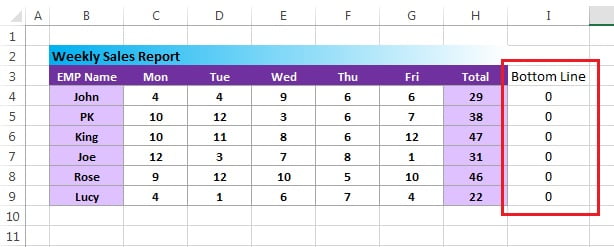
Select the Range “B3:I9”
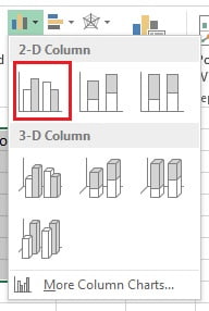
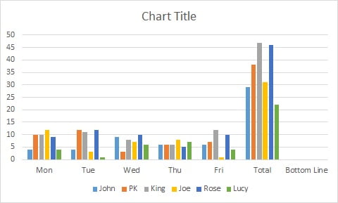
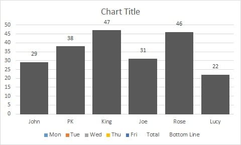
Go to Insert >>Charts>>Column Chart>>Insert a 2D clustered column chart

Insert 2 Clustered Column Chart

After inserting the chart will look like below image

2 Clustered Column Chart

Formatting the Chart

Right click on the chart and click on Select Data.

Select Data Option

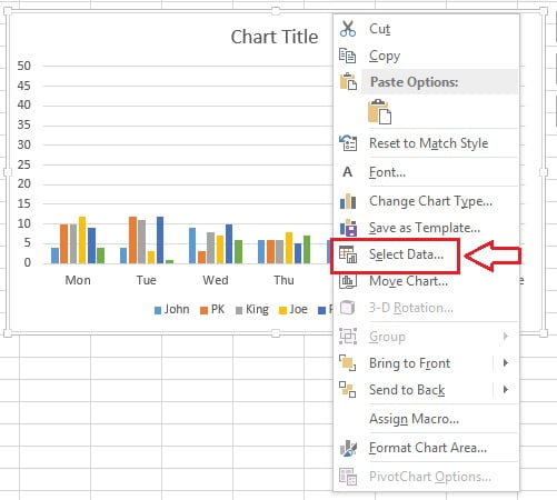
Select Data Source window will be opened.
Click on Switch Row/Column

Select Data Source window

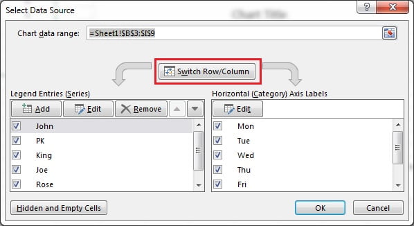
After clicking on Switch Row/Column button our chart will look like below image.

Chart After clicking on Switch Row/Column button

Right click on Total column and click on Change Series Chart Type.

Change Series Chart Type option

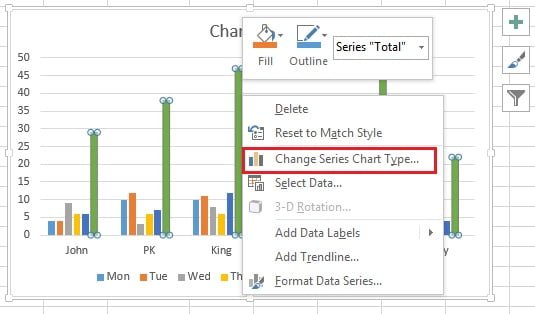
Change Chart type window will be displayed.

Change Chart type window

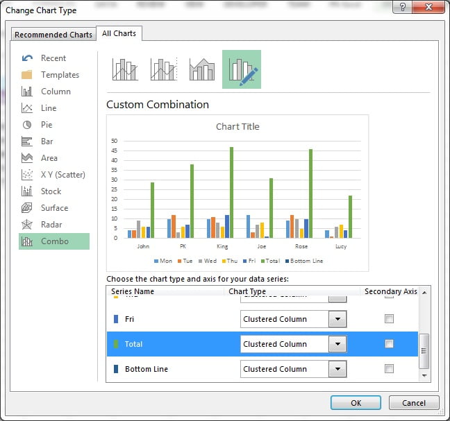
Select the Line chart for Total Series.

Change Chart Type Window

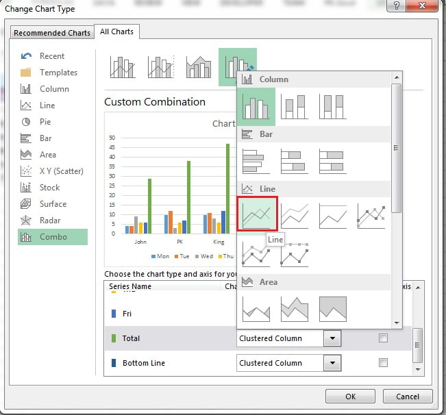
Take the same chart type (Line Chart) to Bottom Line Series also.

Change Chart Type Window

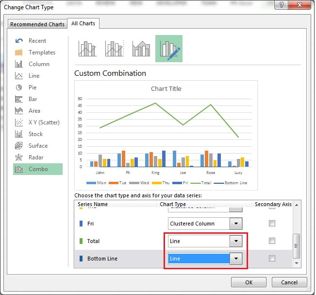
After changing the chart type our chart will look like below image.

After changing the chart type

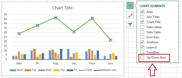
Adding Up/Down Bars

Select the Total line chart (Green Line)
Click on the Chart Elements button (Plus button of chart)
Check the Up/Down Bars

Up/Down Bars Option

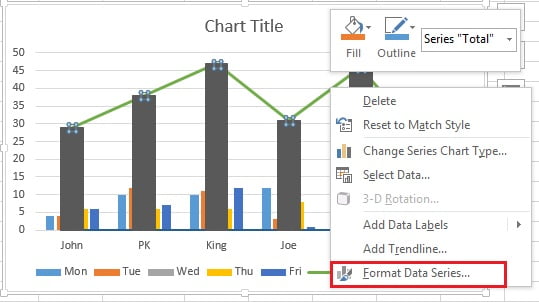
Right click on the line and click on Format Data Series.

Format Data Series option

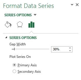
Change the Gap Width around 30% (make sure small columns should go behind the down bars)

Change Gap Width

Right click on the line and click on Add Data Labels.

Add Data Labels

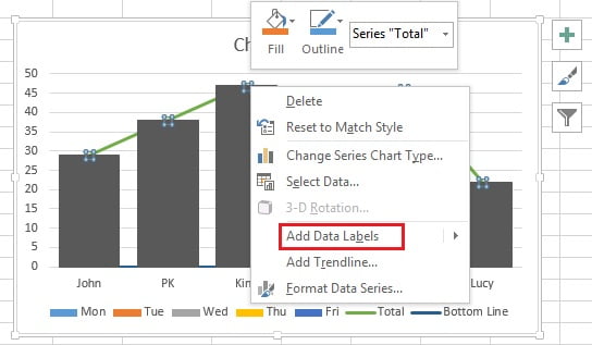
Data labels will be added.
Right click on data label and click on Format Data Labels.

Add Data Labels

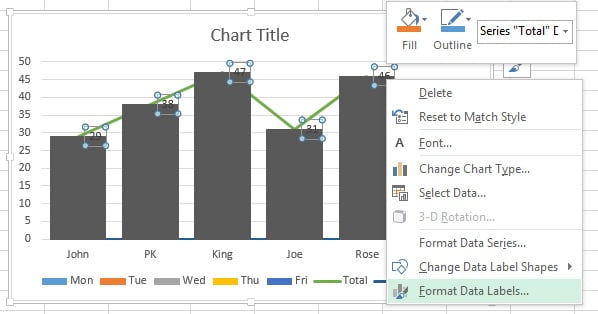
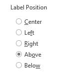
Select Above in Label Position.

Label Position

Go to the Fill and Line option and select No line.

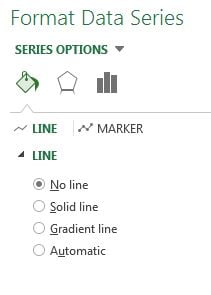
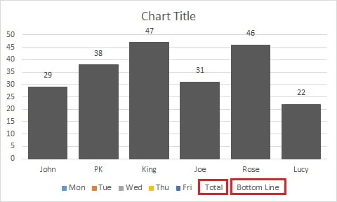
Our chart will look like below given image after choosing the No line for Total Series.

Chart after choosing the No line for Total Series

Delete the Total and Bottom Line in Legends by double clicking and pressing Delete button in your keyboard.

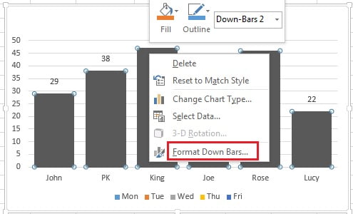
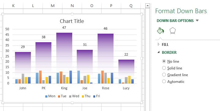
Remove Total and Bottom Line from Legends

Right click on Down Bar (Black Bar) and click on Format Down Bars.

employee-wise sales chart

Fill colors

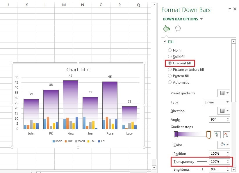
Fill the Gradient Fill in the Down Bars with two Stops.
Select the Type as Linear and put the Angle as 90°.
Keep the color for the First Stop as Purple.
Choose Second Stop color white with 100% Transparency.

Down Bars Formatting

Choose Border for down bars as No line.

Mon-Fri sales trend

Now we can change the data label shapes-

Right click on data label and choose a shape from Change Data Label Shape.

Change Data Label Shape

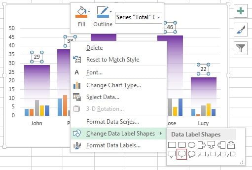
Now change the data label background color as purple.
Change the data label Font color as white.

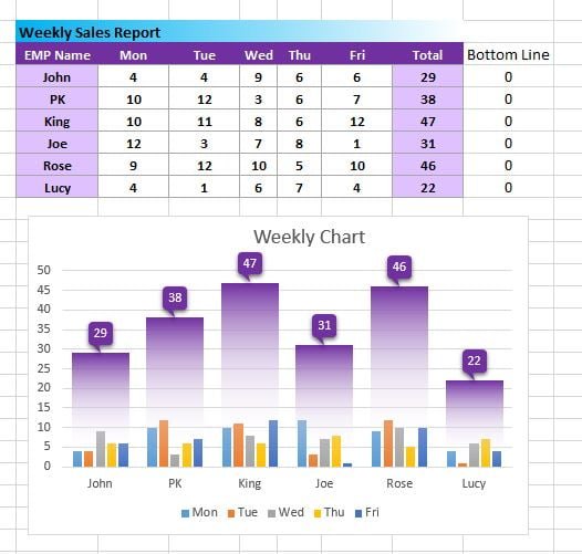
Our weekly Sales chart is ready it will look line below image.

Weekly Sales Chart

Click here to download Weekly Sales Chart.

Watch the video tutorial for Weekly Sales Chart

Meet PK, the founder of PK-AnExcelExpert.com! With over 15 years of experience in Data Visualization, Excel Automation, and dashboard creation. PK is a Microsoft Certified Professional who has a passion for all things in Excel. PK loves to explore new and innovative ways to use Excel and is always eager to share his knowledge with others. With an eye for detail and a commitment to excellence, PK has become a go-to expert in the world of Excel. Whether you’re looking to create stunning visualizations or streamline your workflow with automation, PK has the skills and expertise to help you succeed. Join the many satisfied clients who have benefited from PK’s services and see how he can take your Excel skills to the next level!

Advanced Excel and VBA tutorials

Источник

This tutorial will demonstrate how to create a sales funnel chart in all versions of Excel: 2007, 2010, 2013, 2016, and 2019.

Sales Funnel Chart – Free Template Download

Download our free Sales Funnel Chart Template for Excel.

Download Now

In this Article

Sales Funnel Chart – Free Template Download
Getting Started
How to Create a Sales Funnel Chart in Excel 2019+
Step #1: Create a built-in funnel chart.
Step #2: Recolor the data series.
Step #3: Add the final touches.
How to Create a Sales Funnel Chart in Excel 2007, 2010, 2013, 2016
Step #1: Create a helper column.
Step #2: Set up a stacked bar chart.
Step #3: Hide the helper data series.
Step #4: Reverse the order of the axis categories.
Step #5: Recolor the chart.
Step #6: Adjust the gap width.
Step #7: Add data labels.
Step #8: Remove the redundant chart elements.
Step #9: Shape the chart as a funnel (optional).
Step #10: Insert the inverted pyramid into the funnel chart (optional).
Download Sales Funnel Chart Template

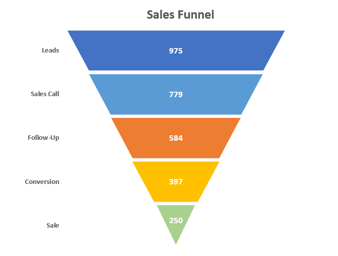
A funnel chart is a graph that dissects different stages of a process, typically sorting the values in descending order (from largest to smallest) in a way that visually looks like a funnel—hence the name.

Funnel charts are commonly used in sales, marketing, and human resources management for analyzing the phases a potential customer or candidate goes through as they move toward the end point, be it signing a deal, purchasing a product, or accepting a job offer.

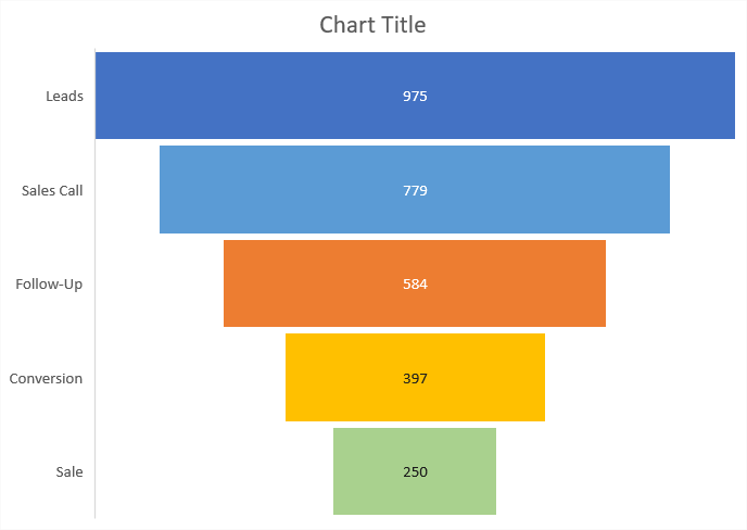
As an example, take a glance at the sales funnel depicting in great detail the customer journey that leads go through to become paying customers—as well as the number of leads that made it through each phase of the sales process, reflected by the width of the bars.

And in this step-by-step tutorial, you will learn how to create this fancy-looking, dynamic funnel chart in Excel, even if you’re a complete newbie.

The funnel chart type was rolled out only in Excel 2019, so those who use earlier versions of Excel have to manually put the graph together on their own. For that reason, this comprehensive tutorial covers both the manual and the built-in methods of building a funnel chart.

Getting Started

To show you the ropes, as you may have already guessed, we are going to anatomize the sales process mentioned before.

Take a peek below at the raw data that will be used for creating the chart:

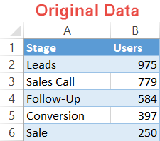
To help you understand the process, we should talk a bit more about the building blocks of the data set:

Stage: This column characterizes the distinct phases of the recruitment process.
Users: This column contains the actual values representing the number of prospects that made it through to a certain stage.

Now it’s time to jump right into action.

How to Create a Sales Funnel Chart in Excel 2019+

Let’s start off by covering the built-in method first, which only takes a few simple steps, for those looking for a quick-and-dirty solution.

However, you should be aware of the price you must pay for automating all the dirty work:

Compatibility issues: The funnel chart type is not available in older versions of Excel, so everyone except for those using Office 365 or Excel 2019 will not be able to see a funnel chart created with this method.
Poor customization: By definition, sticking to chart templates leaves you somewhat shackled by the rigid parameters of Excel defaults, meaning you lose out a lot on customization options.

For that matter, when you know that the file will be shared with a lot of people, you would be better off creating the chart manually from scratch.

But if those issues are of no concern to you, simply take the shortcut outlined below.

Step #1: Create a built-in funnel chart.

Right off the bat, design a default funnel chart.

Highlight the entire cell range containing the stages and values (A1:B6).
Go to the Insert tab.
Select “Insert Waterfall, Funnel, Stock, Surface, or Radar Chart.”
Choose “Funnel.”

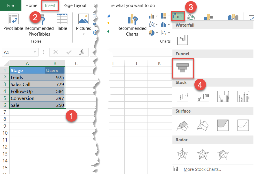
Excel will automatically set up a funnel chart based on the data you fed it:

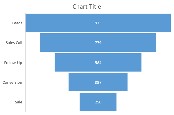
Technically, you have your funnel chart. But you can do a lot better than that by tweaking a just few things to make the chart more pleasing to the eye.

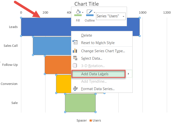
Step #2: Recolor the data series.

Our first step is enhancing the color scheme to transform the chart from dull to eye-catching.

Double-click on the bar representing the data point “Leads” to select it and right-click on it to open a contextual menu.
Click the “Fill” button.
Pick dark blue from the color palette.

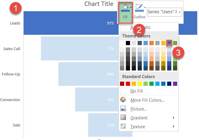
Change the color of the remaining bars by repeating the same process. Eventually, your funnel graph should look like this:

Step #3: Add the final touches.

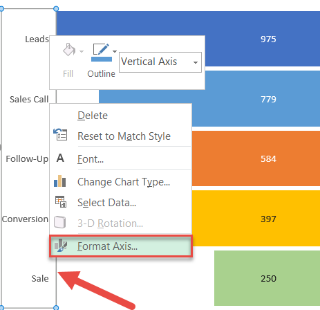
At this stage in the process, you can tweak a few things here and there to make the chart look neat. First, remove the vertical axis border that doesn’t fit into the picture.

To do that, right-click on the vertical axis and select “Format Axis.”

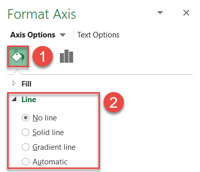
In the task pane, remove the border in just two simple steps:

Go to the Fill & Line tab.
Choose “No line.”

Finally, adjust the color and font of the data labels to help them stand out (Home > Bold > Font Color) and change the chart title.

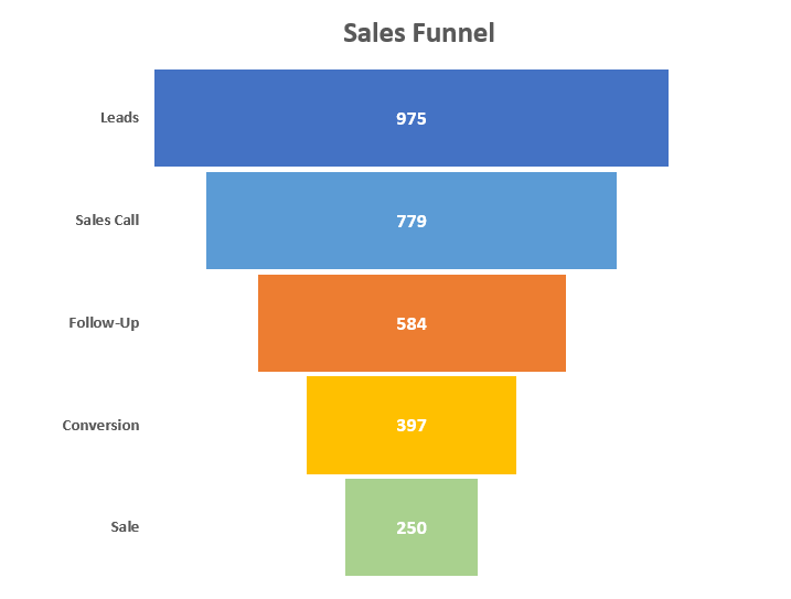
After you have done that, to shape the chart likea funnel (rather than the staggered edges it currently has), skip to Step #9 at the end of the tutorial down below.

How to Create a Sales Funnel Chart in Excel 2007, 2010, 2013, 2016

While we didn’t even have to break a sweat when using the built-in method, it should be obvious that achieving the same result by taking the manual route involves more work on your part.

Regardless of the reasons why you may opt for the manual method—ranging from gaining full control over customization or making the chart compatible with all versions of Excel to simply using an older version of Excel in the first place—in our case, hard work pays off.

Down below, you will find step-by-step instructions covering the process of building this colorful funnel chart in Excel from the ground up.

Step #1: Create a helper column.

At its core, a custom funnel graph is a special hybrid of a center-aligned stacked bar chart. But before we can proceed to build the chart itself, we need to put together some extra data first.

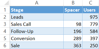
To start with, split the raw data with a spacer column named “Spacer” (column B) that will contain the dummy values for pushing the actual values to the center of the chart plot.

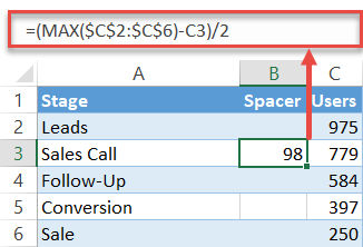
Enter the following formula into the second cell of column Spacer (B3) and copy it down to the end (B6):

=(MAX($C$2:$C$6)-C3)/2

This formula computes a helper value proportional to the number of candidates for each phase to help you center the bars the right way.

At this point, your chart data should be organized this way:

Step #2: Set up a stacked bar chart.

You now have all the data you need to put together a stacked bar chart, the stepping stone to the future funnel graph.

Highlight all the chart data (A1:C6).
Go to the Insert tab.
Click “Insert Column or Bar Chart.”
Choose “Stacked Bar.”

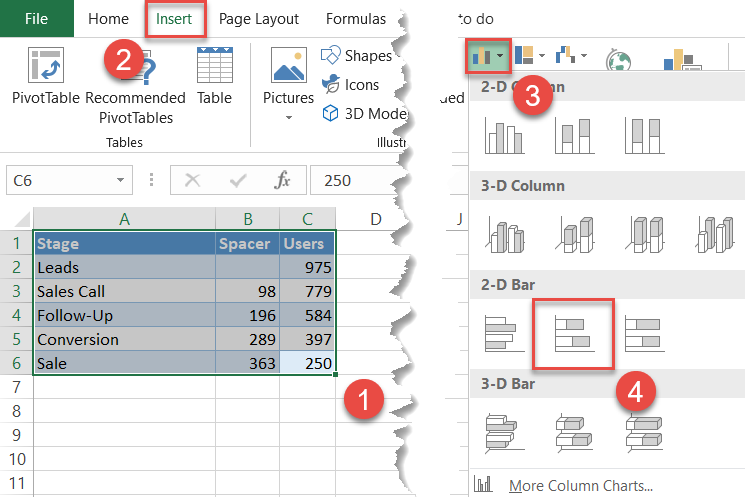
Right away, a simple stacked bar chart will pop up:

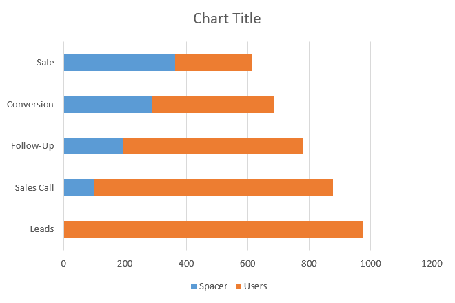
Step #3: Hide the helper data series.

The dummy Series “Spacer” should be hidden, but simply removing it would ruin the entire structure. As a way to work around the issue, make it transparent instead.

Right-click on any of the blue bars representing Series “Spacer” and choose “Format Data Series.”

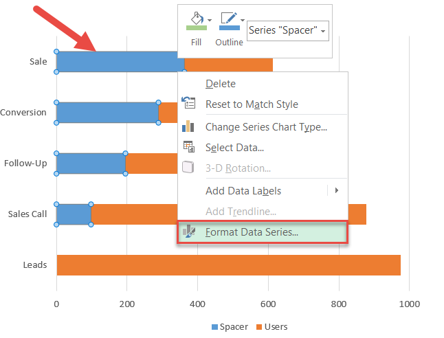
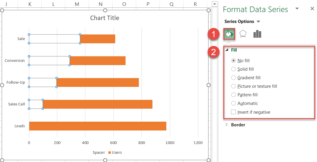
In the Format Data Series task pane, hide the spacer columns:

Navigate to the Fill & Line tab.
Under “Fill,” choose “No fill.”

Step #4: Reverse the order of the axis categories.

In a funnel chart, the broad base at the top gradually morphs into the narrow neck at the bottom, not the other way around. Fortunately, you can easily flip the chart upside down by following a few simple steps.

Right-click on the primary vertical axis and choose “Format Axis.”

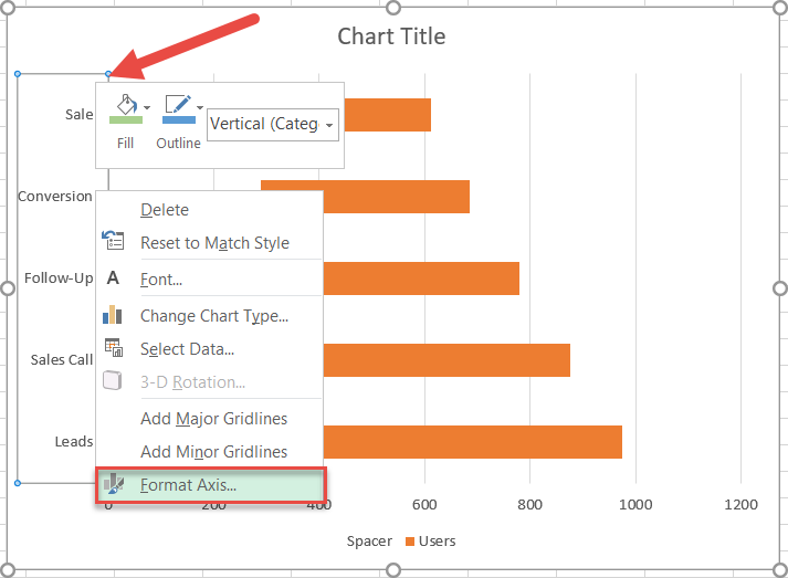
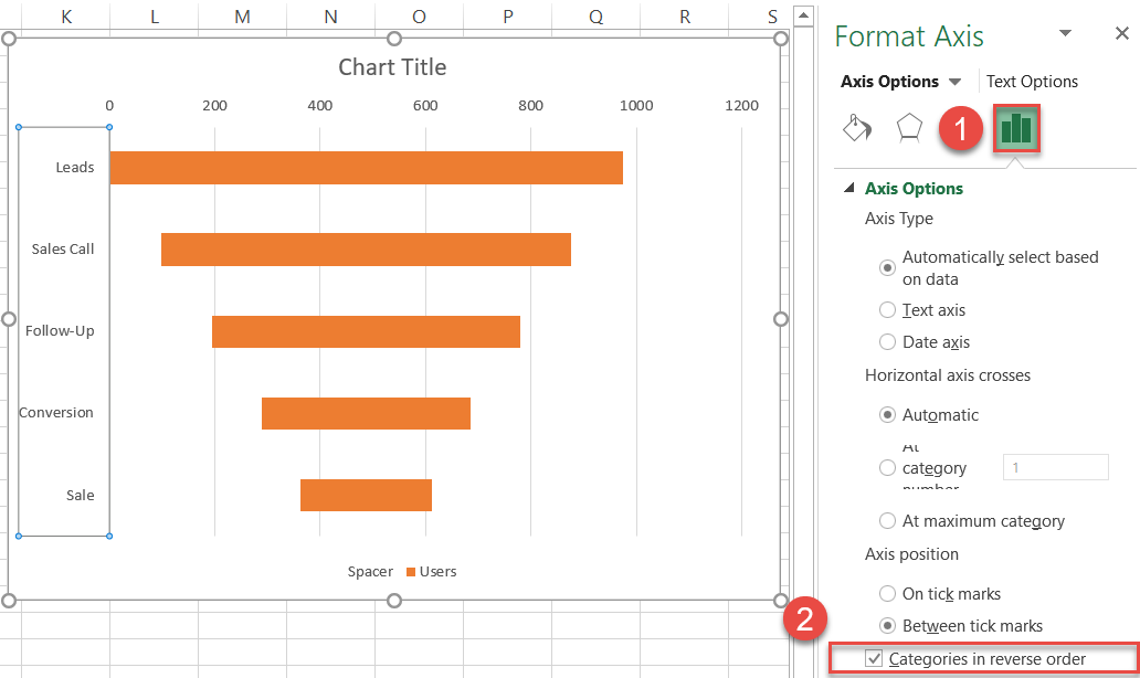
In the task pane, reverse the category order:

Switch to the Axis Options tab.
Check the “Categories in reverse order” box.

Step #5: Recolor the chart.

As you proceed with the next steps, each horizontal bar should be congruent with the color scheme of the finished funnel chart.

To recolor a given data marker, double-click on the horizontal bar you want to change to select that bar in particular, right-click on it, and select “Format Data Point” from the menu that appears.

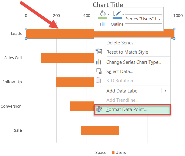
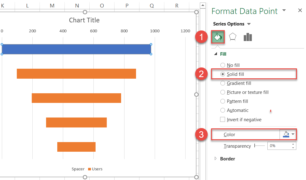
Once the task pane appears, modify the color of that data point by doing the following:

Go to the Fill & Line tab.
Under “Fill,” choose “Solid fill.”
Click the “Fill color” icon and pick dark blue.

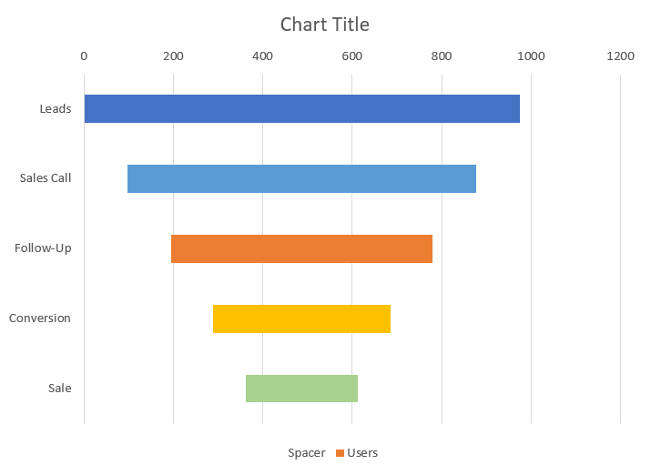
Repeat the same process for the remaining bars. After you have adjusted the color scheme, your chart should resemble something like this:

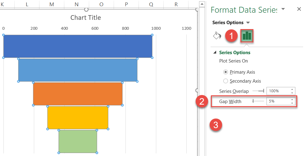
Step #6: Adjust the gap width.

Let’s increase the width of the bars by modifying the gap width of the data series.

Right-click on any horizontal bar, open the Format Data Series task pane, and adjust the value:

Go to the Series Options tab.
Set the Gap Width to “5%.”

Step #7: Add data labels.

To make the chart more informative, add the data labels that display the number of prospects that made it through each stage of the sales process.

Right-click on any of the bars and click “Add Data Labels.”

Step #8: Remove the redundant chart elements.

Finally, clean up the chart area from the elements that have no use for us: the chart legend, the gridlines, and the horizontal axis.

To do that, simply right-click on the chart element you want to get rid of and choose “Delete.”

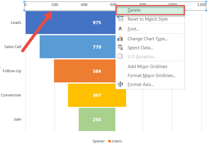
Additionally, remove the axis border (Right-click on the vertical axis > Format Axis > Fill & Line/Fill > Line > No line). Then rewrite the default chart title, and your funnel chart is ready to go!

But there’s more to it. Read on to learn how to visually shape the graph into a funnel.

Step #9: Shape the chart as a funnel (optional).

For those refusing to beat the dead horse of the same rehashed data visuals over and over again, you can trim the horizontal bars to shape the chart into an actual funnel.

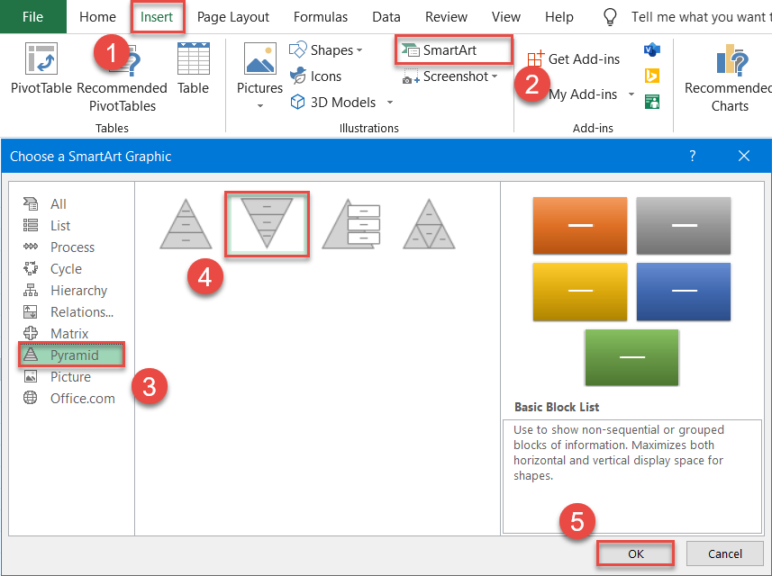
But for the magic to happen, we need to tap into the power of SmartArt graphics. As a jumping-off point, set up an inverted pyramid using the SmartArt feature in Excel.

Go to the Insert tab.
Hit the “SmartArt” button.
In the Choose a SmartArt Graphic dialog box, navigate to the Pyramid tab.
Choose “Inverted Pyramid.”
Click “OK.”

Here is what should pop up instantly on your spreadsheet:

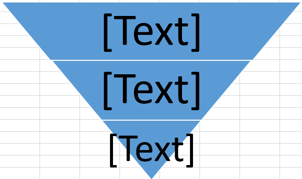
To pull off the trick, the number of pyramid levels should equal the number of categories in the funnel chart—represented by the six stages of the recruitment process.

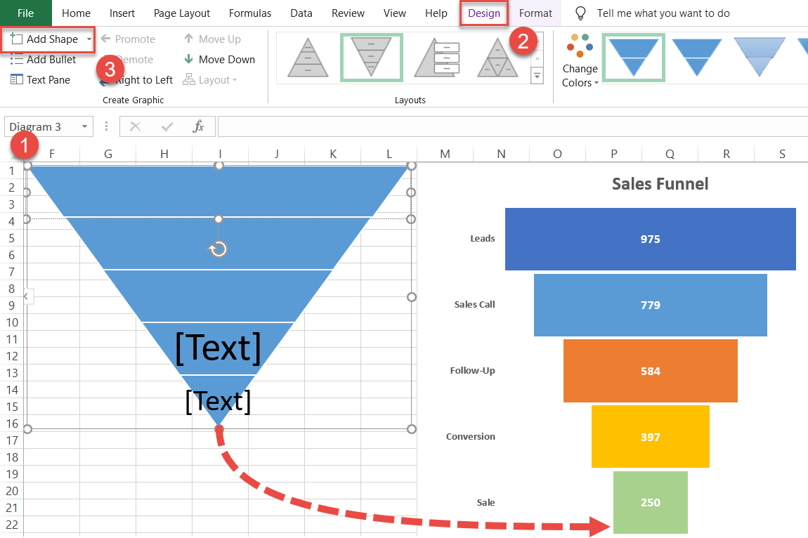
Three down, two to go. To add the pyramid levels we lack, do the following:

Select the inverted pyramid.
Go to the Design tab.
Click “Add Shape” to add an extra level to the pyramid. Repeat the process as many times as you need.

The groundwork has been laid for your streamlined funnel chart. Now, convert the SmartArt graphic into a regular shape so that you can paste it into the funnel chart.

Select the entire inverted pyramid, right-click on it, and choose “Convert to Shapes.”

Finally, replicate the color scheme of the funnel chart.

To recolor one level of the pyramid, double-click on the level to select it, then right-click on it and select “Format Shape.”

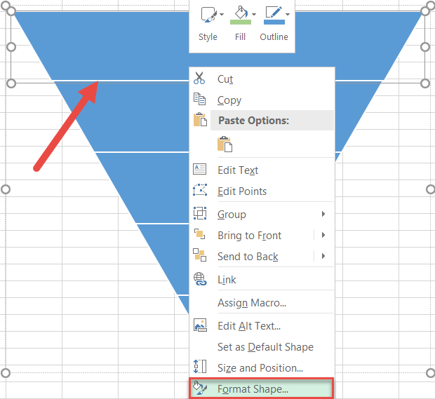
In the Format Shape task pane, go to the Fill & Line tab. Under “Fill,” choose “Solid fill” and pick the color you want.

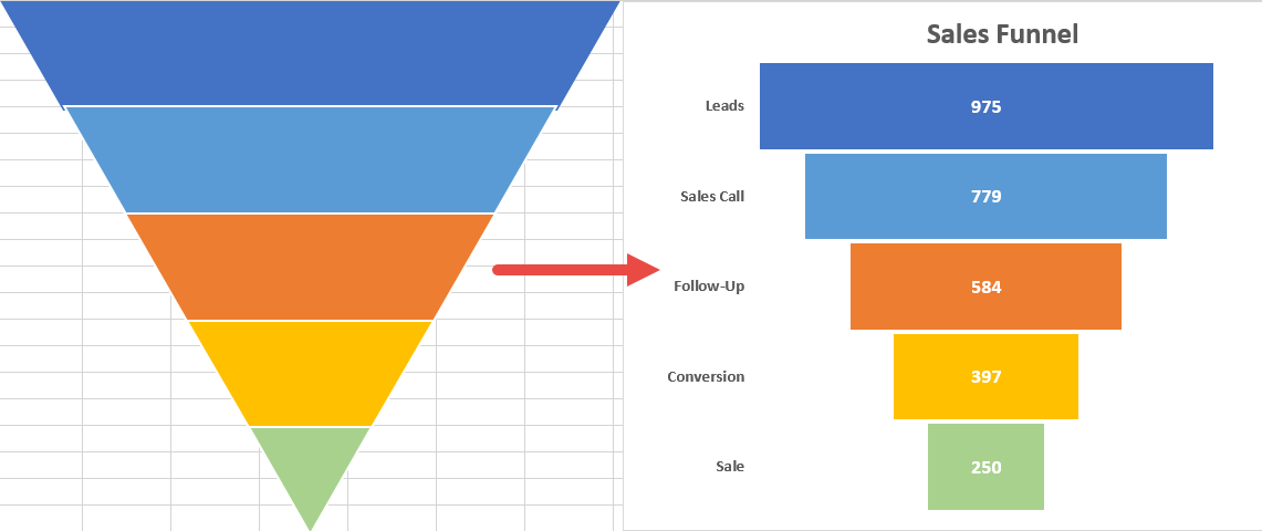
For your convenience, here is the inverted pyramid you should end up with by the end of this phase:

Step #10: Insert the inverted pyramid into the funnel chart (optional).

Having set up the pyramid, insert the shape level by level into the funnel graph by doing the following:

Double-click on the top level of the inverted pyramid, right-click on it, and choose “Copy” or press the key combination Ctrl + C.

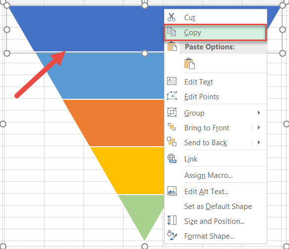
With that level copied to the clipboard, select the corresponding horizontal bar in the funnel chart and open the Format Data Point task pane (Double-click > Right-click > Format Data Point).

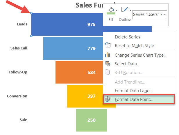
Now, add the copied pyramid level as the “texture fill” of the data point:

Go to the Fill & Line tab.
Change “Fill” to “Picture or texture fill.”
Under “Picture source,” choose “Clipboard.”

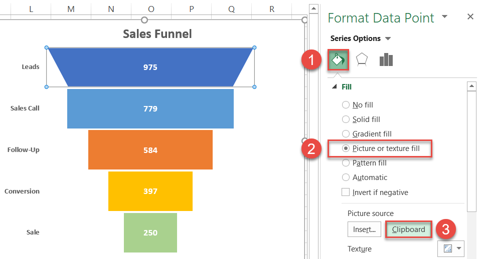
Repeat the process for every single bar of the funnel chart. Ta-da! You have just crossed the finish line and have a stunning sales funnel chart ready to blow everyone away.

Download Sales Funnel Chart Template

Download our free Sales Funnel Chart Template for Excel.

Download Now

Источник

Charts and Graphs, Cool Infographics & Data Visualizations, VBA Macros

Last updated on May 9, 2012

Chandoo

Finally, I got some time to sit down and do what I love most – write a blog post to make you awesome in Excel. After a whirlwind trip to Sydney, I am back in India to spend few days with my kids & wife before rushing to Australia to run 2nd leg of my training programs (in Perth, Melbourne & Brisbane). I did 2 sessions in Sydney – one for KPMG and other for public and both went very well. We got lots of positive feedback and people really loved it. I am saving the details for another post, but today lets talk about Interactive Sales Chart using Excel.

Take a look at the Interactive Sales Chart

First, take a look at interactive sales chart. Today, you will learn how to build this using Excel.

Inspiration for this chart

Before we learn how you can create such a chart, let me tell where the inspiration came from. Yesterday, Persol, a forum member asked, How to make an info-radar chart, where he mentioned the below chart from Good.is

[Click here to play with this chart]

While I took inspiration from the above chart, I replaced the radar chart with a regular column chart (as column charts are easier to read) and modified the data to a sales data set.

How to create interactive sales chart in Excel?

First, take a look at the data

The sales data for this chart looked like this:

I have set up this data in an Excel Table called as tblSales so that it is easier to write formulas.

The formulas

To calculate various values in the chart, we use ample doses of SUMIFS formula.

The Interactivity

When you click on any year, region or product name, we run worksheet_seletionchange event. This tells our calculation engine which year, region & product are chosen. Then the formulas would (re)calculate the data for charts. This updates the charts & conditional formats.

[Related: Show on-demand details in Excel using VBA]

Here is how the interactive chart works:

How to create interactive charts like this – Video

Since the actual mechanics of this are quite elaborate, I made a short video (15 min) explaining how various parts of this chart work. Please watch it below.

[You can watch the video on our Youtube channel too]

Download Interactive Sales Chart Workbook

Click here to download the workbook & play with it. Examine the macros & formulas to learn more.

How do you like this chart?

I really liked Good.is chart and wanted to see how much of it we can do in Excel. It was a fun exercise. I have noticed that such charts excite people (decision makers too) and make your reports fun.

What about you? How do you like the interactive sales chart? What additions / modifications would you do to it? Please share your thoughts using comments.

Create Interactive Charts using Excel

Interactive charts are one my favorite visualizations. They let users play with the chart & decide what they want. So, naturally I write about them every now and then. Please go thru these examples if you want to learn various interactive charting techniques in Excel.

Show top x values in a chart interactively
Interactive dashboard using hyperlinks
Suicides vs. Murders – Interactive Excel Chart
Create a quick dynamic chart in Excel
Interactive charts that leave your boss drooling
More on Interactive Charts

I also recommend enrolling in our Excel + VBA Class if you want to learn these techniques and create stunning reports & charts. Click here to learn more about our Excel + VBA training program.

Share this tip with your colleagues

Excel and Power BI tips - Chandoo.org Newsletter

Get FREE Excel + Power BI Tips

Simple, fun and useful emails, once per week.

Learn & be awesome.

95 Comments
Ask a question or say something…
Tagged under

charting, charts, column charts, downloads, dynamic charts, excel tables, interactive, interactive charts, Learn Excel, macros, Microsoft Excel Conditional Formatting, Microsoft Excel Formulas, screencasts, sumifs
Category:

Charts and Graphs, Cool Infographics & Data Visualizations, VBA Macros

Welcome to Chandoo.org

Thank you so much for visiting. My aim is to make you awesome in Excel & Power BI. I do this by sharing videos, tips, examples and downloads on this website. There are more than 1,000 pages with all things Excel, Power BI, Dashboards & VBA here. Go ahead and spend few minutes to be AWESOME.

Read my story • FREE Excel tips book

Excel School made me great at work.

 5/5

Excel formula list - 100+ examples and howto guide for you

From simple to complex, there is a formula for every occasion. Check out the list now.

Calendars, invoices, trackers and much more. All free, fun and fantastic.

Power Query, Data model, DAX, Filters, Slicers, Conditional formats and beautiful charts. It’s all here.

Still on fence about Power BI? In this getting started guide, learn what is Power BI, how to get it and how to create your first report from scratch.

Related Tips

95 Responses to “Interactive Sales Chart using MS Excel ”

Peter says:

Great chart Chandoo,
It would be nice to make a additional selection where you can chose what kind of chart the data will be viewed in. Bars, Lines etc.

Peter
- - Peter says:
    
    Chandoo,
    
    Thnak you for the link. Will look into it.
Matt says:

Outstanding!
Andrew says:

Damn I want to do this so bad! But Excel 2003 doesn’t seem to work with this.
- Lubos says:
  
  Andrew,
  
  I use Excel 2003 too. All you need to do is replace the SUMIFS formulas in sheet Calculation with formulas with SUMPRODUCT. I’m sure Chandoo explained it somewhere.
  
  Excel 2003 doesn’t support SUMIFS. But in my opinion SUMPRODUCT is even better.
  
  It takes some time to rewrite the formulas but as a result all the interactivity will work.
  
  Lubos
thats really awesome & simple thanks for good working and good ideas.
Christian says:

Thank Persol & Chandoo,

Awesome chart.

My critique would include a lack of comparison year to year — the graph is showing many years, but lacks the ability to visualise/ measure the change. Quite static in many repects.
I know they are showing the level of interest in issues realtive to each other, but with so many years history I think they could have added more value by allowing the graph to not only show actual yearly values — but perhaps to see variance between two particular years, or the variance between the three party categories in a particular year.

Lovely visualisation and interactivity, value add potential for analysis if I were to make suggestion for improvement.

Cheers — and see you in Bris Vegas (Brisbane)
- I agree. We can take the same data and visualize it differently so the focus will be on yearly trends. Would you like to give it a try and share the workbook with all of us?
Jez says:

Awesome — as usual — and I have adopted many of the techniques from this blog — but strangely (and I am showing my ignorance a bit here) but I can follow understand and implement the techniques in the example however I have no idea how to «switch off» the area outside A1:M25 — how is this done ? ie. I cannot select cell P12 — why not ? It doesn’t even show P as a column heading ?!! What am I missing ?
- Matt Nuttall says:
  
  It has something to do w/ the scroll area. If you open VBA, select the worksheet «Interactive Sales Chart» on the side and change the Scroll Area to A1:Z500 (for example) it will open up other rows/columns. It was blank to begin with and returns blank after you hit enter.
  - Jay says:
    
    Actually, It was the Property «StandardWidth» being set to 0 (which apparently sizes the sheet to end with the last used column). Setting that to 8.43 (or whatever the other sheets are set to) exposes additional columns Setting it back to 0 returns it to the Original behavior. This is a cool new «tip» for me to know!
- Thank you. It is really simple once you know it.
  1. Just select all the columns from P till end (select column P, then CTRL+SHIFT+End)
  2. Hide columns
  3. Select rows 26 till end (select row 26, CTRL+SHIFT+Down)
  4. Hide rows.
  5. and we are done.
  - Matt Nuttall says:
    
    Even easier than what I was thinking!
    
    Nice tip.
    - Nick says:
      
      Awesome stuff. Was trying to figure out how he did that, expected it to be harder.
  - Jez says:
    
    Doh !! Lol 🙂
    
    Thanks Chandoo
Fred says:

Nice Chart! I guess I can use it at work.
Kiev says:

This is really a great post, i love it so much, it can definitely can be used at work. The most important thing i learn from your post is always open to new ideas. Thank you so much.
Linda says:

Thanks for the great post. One thing I do not understand. How do you get the link between the region-wise breakup graph in the Calculations and the graphic on the chart?

Thanks,

Linda
- - Linda says:
    
    Thank you, works beautifully
Waseem says:

Hi Chandoo

This is great stuff and I have already started copying it for my work. Just one question please. How do we change Bar color (in bar chart) when we select a product along x — axis?
- Fred says:
  
  you will need to create 2 rows of the same chosen data set. Say you have picked 2011 and a set of data would show up. you want to duplicate one more set.
  
  First set: the bars not click would become zero. So only the chosen bar would stand out and give it a color.
  Second set: the bars not click would show their figures. But the bar chosen would become zero. So you give the bars another set of color.
  
  when you create the graph you will need to specify both data line. One with only the bar of you choice showing black, in this example. And the bars not chosen would become orange/red.
  
  hope this help.
  - Waseem says:
    
    Great. thanks a lot Fred. I’m gonna try it now.
xsaed says:

i’m using excel 2007, the camera function is not working… i.e the inline charts are not showing in the interactive chart…
what should i do?
one other thing, how to select hidden columns to unhide it if i use ctrl+end?
Rahul says:

Hi Chandoo

Nice post, Really loved it and curious to know what next to come. I just noticed one thing that I can’t able to see your last month articles like u posted the articles in month of April and march. When I click on page 2, I found very old articles that u posted it in month of Feb. However, it should come the April’s and march month article. Can you fix this problem as I need an article which is written on VBA.

Thanks in advance.
- Rahul says:
  
  Sorry for the above post. Now I can see your previous post. I don’t know why earlier i was not to see the post. Thanx
Waseem says:

Chandoo I have another scenario to deal with. Just like we click in the rows to pick a particular year, can we select multiple entries? Actually I need to put certain products along this axis and my objective is to produce results for one product as well as selecting multiple products (the way it works and looks like in your worksheet).

Thanks for making our life easier 🙂
I love this blog and can’t get enough of every aspect of it. You are a fabulously talented writer and manage to make everything so relatable. You are so good at this in fact, that sometimes while reading I feel like our hearts and minds become one and basically I feel as if I am reading my own thoughts.
Lubos says:

Chandoo, this is great. I use this technique already.
However I could learn somenting new AGAIN. This little feature SHOW/HIDE HELP is a great idea how to get rid of the information which is firstly important to know but later redundant.
Thanks for the idea, I will use that in my dashboards.

Lubos
[…] Create a cool interactive Sales Chart […]
Neil says:

Very impressive, both in terms of the output and how it’s put together.

My only comment would be to include an additional line of code that re-calculates the calculations sheet, for those of us that have calculation set to manual by default.
Lionel says:

Chandoo,

Firstly, impressive, love your work.

I have added more regions, but how do I move the «Products» down 4 rows and make the chart bigger on the Interactive chart page. Also, the show hide help doesn’t work for me.

Lionel
Paul says:

Love this chart!

How would I add more products? is this easy to do?
Sunil says:

How do i get my bars started at the same place.. if i select all regions my bars start at one place and if i select north the graph starts at a different place on the X axis and if i select south it gets started at a different place on the X axis.. this is creating problem for me to overlap the two charts .. please advice
Neha says:

Hi Chandoo,
Awesome tutorial. Never though one could learn it so fast.
Narendra says:

Hi Chandoo,

Greate charts !!!
Chintan Parmar says:

Hi,

Can We Create Political Climate chart in excel….. I tried lot but not able to get success in this chart…..

Would u please sugget about the same….
Chintan Parmar says:

Hi,
Can We Create Political Climate chart in excel….. I tried lot but not able to get success in this chart…..
Would u please sugget about the same….
- @Chintan Parmar
  
  Can you post a link to an example
[…] «chart» macroClick OKRepeat above steps with the remaining rectangles.Recommended posts:Interactive Sales Chart using MS Excel Download excel *.xlsm fileChart.xlsmNo related posts.Recommended categoriesAutomateChartsExcelvba […]
frank says:

Hi,

I love your charts. How can I do this chart with more than 1 chart value. On your chart there’s only sales for the products, but what if I want sales and revenue numbers on the same chart? Also can I just delete the region part of the chart? I just want it to have the products and year with sales and revenue data.?
- Ursula says:
  
  Hi Frank (or others), I have the same question; I’d like to include more data on the same chart, I don’t seen an answer here, did you work it out perhaps? If so, would you share what you did please?
  
  Thanks!
OPS says:

Hi,

Something wrong with the video?
Can you please solve this….
[…] Interactive sales chart using Excel […]
Ursula says:

This is a super chart, and I would really like to work something like this out for data I’m collecting for my PhD, however, as in my reply to Frank’s post above, I would not only to like to visualise one variable at a time; so to use the example given in this video I would like to visualise sales as well as other variables like demand and stock of each of the products simultaneously on the chart; could someone help me in doing that please?

Also, I would prefer to have a line graph instead of bars…?

Any help would be much appreciated. Many thanks!
Venkat says:

Thanks a ton Chandoo. Interactive chart looks simple but awesome. I am more convinced to join your class

Keep posting
Pulkit says:

Great work Chandoo!

I am really thrilled to see your work, I am learning new things which i could not believe i can do with the spreadsheet!

This interactive dashboard looks really fabulous, I will get my hands on it. A big thanks and keep up the good work!
Nishant says:

Hi chandoo,

A very good tutorial and very helpful video made by you. Thank you for sharing all this. I will be working on demand analysis, using the logic you have explained for Interactive chart. Hope I am able excute it the same way you have done it, or else I will be back with my mails flooding in your inbox 🙂
Have a great day ahead.
Nishant
Reginald Vaz says:

Awesome…The Interactive Sales Chart
Thanks Chandoo for sharing this…
Vikas Dhand says:

Dear Chandoo, First of all i would like to thank you for creating such a wonderfull forum on excel. I was having very basic knowledge of Excel, but by following ur blog i have become excel master in my Office. Now i teach excel to my Assistants who are supposed to make reports.
I am having query related to this interactive sales chart. In Calculations sheet please let me know about =valueproductpicked, valueregionpicked. Is it macro or sum new formula. also how it is connected to Interactive sales chart file where «pick an year» «region and «product are selected.
Santhosh says:

Hi Chandoo,
I would like to thank you for creating such a wonderful chart by effectively using the simple functions in excel.I have a question on the data labels.When data label is added in the chart and we choose a «yea»r and then if we choose a «region» #N/A’s appear and data labels disappear.Any thoughts around that.
- Kylee says:
  
  Hi Chandoo,
  I am also puzzled like Santhosh about how to make the data labels work. Can you shed your wisdom please?
  Thanks very much, Kylee.
AKhilesh says:

Dear Chandoo,
This Video is not working and giving some error. Can you Upload it again.
Thanks,
- Hi Akhilesh, Can you try again. It is working alright for me.
  - AKhilesh says:
    
    I think there was some problem with Firefox. It was working fine in Chrome.
    Thanks.
Paul says:

Great site, Great article, but I am coming unstuck as I build my formula.

=SUMIFS(tblOverview[Jan],tblOverview[Business],valGroup,tblOverview[Category],valHardware)

Works a treat (Wow, so impressed) but adding a new condition

=SUMIFS(tblOverview[Jan],tblOverview[Business],valGroup,tblOverview[Category],valHardware,o28,valGroup) falls over with a #Value error.

Putting o28=valGroup in a different cell gets the result TRUE.

If I click [Show calculation steps] the formula appears to resolve (with the ranges and values being returned as I would expect) and it says «the next evaluation will result in an error» which, I guess, is the sumifs part.

Help! 🙂
- Thank you Paul. Please note that all data columns must be of same size fo SUMIFS to work. In your case, 028 is a single cell, and SUMIFS cannot evaluate the condition o28=valGroup when rest of the conditions are looking in a range.
  - Paul says:
    
    Thanks Chandoo, ValGroup is also a single cell (from your article how to click on a chart axis to change the chart data). I did try replacing o28 with 025:o33 but received the same error so that threw me off the scent a bit. I’ll keep playing with it as this is a powerful formula you have introduced to me.
    - Paul says:
      
      Please do not make further replies to this post ~ my logic is flawed and the result would be stupid 🙂 (Does not stop the concept being brilliant, Thanks again).
[…] blog, so it was hard to pick just one for this list of favourites. However, I finally selected this interactive sales chart example, because it incorporates several useful […]
Kylee says:

Hi Chandoo,
Absolutely love the design and simplicity of this graph. Half spent half of today getting my head around it to make it work for my data. Fifth attempte = sucess 🙂
One question, how could we add budgeted sales for the applicable year to show as a bullet point style graph superimposed over the actual sales bar graph?
Thanks so much, Kylee.
Rodrigo says:

Hi Chandoo,
you have a lovely website and system of learning. But i was stuying this sheet and got frustrated while constructing a dashboard on my own. How can i use the same effect or use drop-down lists, to this situation:
Its for my Balanced Scorecard sheet, so i have a number of indicators and its values. The vary by year, perspective and indicator. So i wanted to select: In the finance perspective, the wallet share indicator, of the 2012 year. So it would select the values (Jan, Fev, Mar…) and mount a graphic.
abc says:

Hi chandoo,
How to change format cell when it’s clicked.
Iuliana says:

Hi Chandoo,

first thank you for this example but..i am trying to build this with different table names etc ..would like to know the TRUE result next to the year on sheet with calculation..what is the aim of that?

Thank you,
I
Sriram says:

Hi
This is really splendid work — simple but very powerful. I am adopting this to present a few results using this concept. The modifications are
1.instead of presenting just one series I am presenting 2 series -clustered bar graphs
2. it is comparing certain distributions region wise (instead of year wise).

Now, all is well until I prepare the overlapping graphs. There instead of all the null values being hidden I get an expanding graph with gaps. By the end of the process the graph display becomes miniscule. Any workaround? — what am I missing?
Sandeep says:

I used the technique expressed here and derived the results I wanted. Thanks for the education and the entertainment you provide here.
I still want to raise a query here being that based on the SUMIFS which generates the chart data (excluding the #NAs) as per different values picked up the graphs draw but their colour schemes etc. have to be painfully corrected to ensure consistency across. Is there a way to ensure we do it once for all the combinations?
I tried copy-pasting formats across but that does not work in Excel 2007.
Regards,
Sandeep
- Pharasi says:
  
  Hi Sandeep,
  
  Can you please help me in making exactly this kind of a chart with my data. I am trying to replace it with my data but the chart area isnt big enough.
  
  Thank you
  Kartika
Joe says:

Hello, I am using excel 2007, the file downloaded looks does not works on it. Not sure if you could have 2007 version? That would be great! Thanks.
Its like you read my thoughts! You seem to grasp so much approximately this, like you wrote the e book in it or something.
I feel that you just can do with some p.c. to power the message home a bit, however
instead of that, that is excellent blog.
An excellent read. I will certainly be back.
Carlos says:

please correct me if im wrong but, it would it not be easier if u used a pivot table instead of the sumif?
Carlos says:

UPS, forgot the question, the part i was unsure of was the macro that runs when you click on a year a product or a region..
Ray says:

Hello Chandoo,

Thank you for the example, it’s very useful for me.
But I want to know how to build a Marco that display what you select? for example you select year 2001, then it shows in the calculation sheet.

Thank you in advance
Ray
Daniel says:

Hi Chandoo, GREAT graph and great site!!!! I have a question on the data labels. When data label is added in the chart and we select a “year» and then if we choose a “region” #N/A’s appear and data labels disappear. Any thoughts on this? Thanks and hugs from Argentina.
[…] chandoo.org/wp/2012/05/09/interactive-sales-chart-in-excel/ to get the excel workbook and know more about this. Interactive Sales chart using Mi… Video […]
Kirk Williams says:

Love the video and chart you make it seem simple, but it’s the thought, how can I do it in Excel that’s the real take away. Don’t let anyone say it can’t be done.
Kay says:

Love this Dashboard…
I have a issue…When I add a hyperlink to other Sheet, the Error’1004′: The item with the specifed name wasn’t found.

How can I fix it?

Please and Thanks
- Kerem says:
  
  Hello Kay;
  
  I have the same problem, did you find a solution to your problem?
  
  By the way Chandoo, thanks for the great site and great tips…
  
  Thanks,
  - Kerem says:
    
    Hello Again;
    
    Within minutes I found the right phrase to put into google «Application.Intersect hyperlink error 1004» to give me the correct results; and found out changing ActiveCell to Target does the trick. I can share the link if linking to some other site is ok.
Manfred says:

Hi Chandoo.

Excellente dashboard but I have a problem. I´m using Excel for Mac 2011 and it gives me an error with the macro (error 424). It seems to be something related to «ActiveCell.Value» but I don´t know how to fix it. Could you help me?
Sebastian says:

Hello, I did the dashboard and I understood everything except the vba code, could you explain it to me in simple words, the steps that you did? in case you dont remember, specialy the application.intersect I searched for it but still dont understands

Thank you so much you are super helpful and kind with us excel noobs 🙂

Private Sub Worksheet_SelectionChange(ByVal Target As Range)

If Not Application.Intersect(ActiveCell, [plistyear]) Is Nothing Then
[valyearp] = ActiveCell.Value
ElseIf Not Application.Intersect(ActiveCell, [plistReg]) Is Nothing Then
[valregp] = ActiveCell.Value
ElseIf Not Application.Intersect(ActiveCell, [plistProd]) Is Nothing Then
[valprodp] = ActiveCell.Value
End If
End Sub
Farzaneh says:

Hi Everyone,
I was trying to find a Budget Gap analysis template or Dashboard, is there anything here in this website, Thank you so much! 🙂
Ryan says:

Chandoo thank you for sharing. This is a killer interactive chart! I am working on adapting the model to support my product offering. We retire products and introduce new products. Given this situation, the number of products displayed would differ from year to year. Can suggest a solution to dynamically display the products for a given year?
CHAITANYA says:

hI CHANDOO…HOW ARE YOU ABLE TO GET THE VALUES IN D4 AND D5 IN CLACULATION SHEET BASED ON THE SELECTION MADE IN THE CHART? CAN YOU EXPLAIN THAT PART?
Anshul Singhal says:

Hi Chandoo,

First of all I want to thank you for enlighten me with all nuts and bolts of excel as I am following you from last couple of years. Though this is my first comment on your website.

This particular article is great as always and I have learned a lot from this as well. However just want to add one point that it would be great to create this interactive chart without the use of macro as many people including me don’t possess technical skills to write down the same. I try by myself to modify the same and pleased to share that it can be done without macro as well and I am sure you know this better than me.

Once again thank you so much for such a lovely blog.
I love the ways you organized the chart and using color. Thank you a lot, wish you more success
Archana says:

Very useful and interactive charts Chandoo.. Amidst the Powerpoint presentation, you have proved even the more vague excel sheets also could be in a presentable format. I just tried to have a look into your sales chart, however the macro does not run due to missing objects. Could you please check
Juvabelle Peptide Cream says:

This design is spectacular! You obviously know how to keep a reader
amused. Between your wit and your videos, I was almost moved to start my own blog (well,
almost…HaHa!) Fantastic job. I really enjoyed what you had to say,
and more than that, how you presented it.
Too cool!
brian says:

Im using Excel 2016 on a mac and the selection of years, products or regions gives me a 424 error… object required.
Seems that the mac version doesn’t like:
[valYearPicked] = Active.cell.Value

Not sure it’s picking up on where to get the[valYearPicked] data from…
any suggestions?
brian says:

Sorry that was a typo… it’s how you have it in yours
[valYearPicked] = ActiveCell.Value
brian says:

nevermind — figured it out. With Excel 2016 on a mac you have to specify the object:
sheets(«calculations»).[valYearPicked] = activecell.value
Chip Bender says:

I tried the link supplied to download the Excel example spreadsheet but it indicated the site could not be reached. I would really have liked to see this spreadsheet as I find it very fascinating on how the coding and processes would be performed.
- Hi Chip
  
  Can you please try again. I just checked and it works.

Источник

I am currently working on creating a sales pipeline management dashboard. I have all the data in place and now I am looking for some visualization to create the dashboard. One of the charts that I absolutely want in there is a sales funnel chart.

What is a Sales Funnel?

In any sales process, there are stages. A typical sales stage could look something as shown below:

Opportunity Identified –> Validated –> Qualified –> Proposal –> Win/Loss

If you think about the numbers, you would realize that this forms a sales funnel.

Many opportunities are ‘identified’, but only a part of it is in the ‘Validated’ category, and even lesser ends up as a potential lead.

In the end, there is only a handful of deals that are either won or lost.

If you try and visualize it, it would look something as shown below: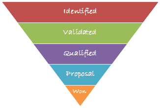

Now let’s recreate this in Sales Funnel Chart Template in Excel.

Download the Sales Funnel Chart Template to follow along

Watch Video – Creating a Sales Funnel Chart in Excel

Sales Funnel Chart Template in Excel

Lets first have a look at the data:

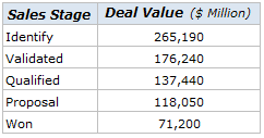
Here are the steps to create the sales funnel chart in Excel:

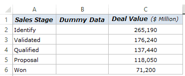
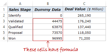
Arrange the data. I use the same dataset, as shown above, but have inserted an additional column between sales stage and deal value columns.
In the dummy data column, enter 0 in B2, and use the following formula in the remaining cells (B3:B6)
```
=(LARGE($C$2:$C$6,1)-C3)/2
```

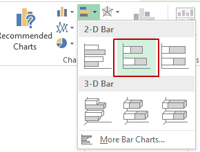
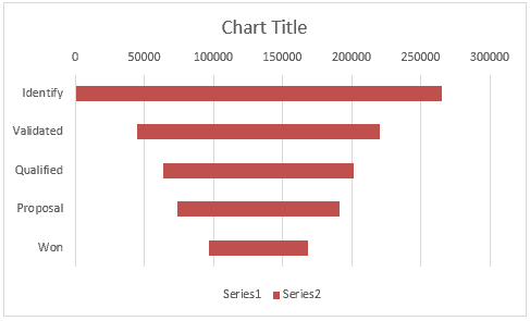
Select the data (A2:C6), and go to Insert –> Charts –> Insert Bar Chart –> Stacked Bar.
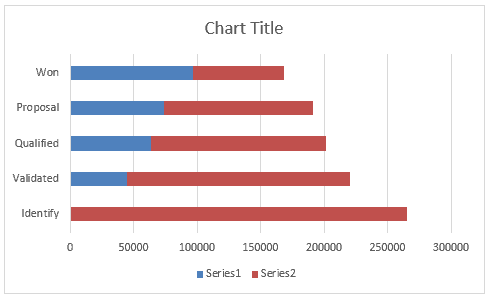
The above steps creates a stacked bar chart as shown below:
Select the vertical axis and press Control +1 (or right click and select Format Axis). In the Format Axis pane, within Axis Options, select categories in reverse order. This would reverse the order of the chart so that you have the ‘Identified’ stage bar at the top.
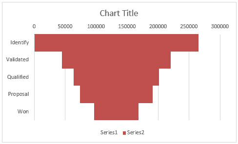
Select the blue bar (which is of dummy data) and make its color transparent
Select the red bars, and press Control +1 (or right click and select Format Axis). In the Format Data series pane, select Series Options and change Gap Width to 0%. This would remove the gap between these bars
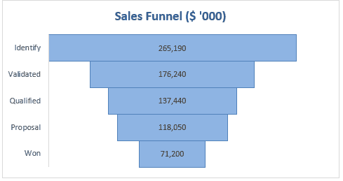
That’s it. Now remove the chart junk and format your chart to look awesome. Here are some steps I took to format it:
- Removed the legend and horizontal axis
- Changed Chart Title to ‘Sales Funnel’
- Changed bar colors to blue
- Added a border to the bars
- Added data labels
- Removed gridlines

Download the Sales Funnel Template

That’s all right Sumit. But where is the Dashboard?

I am working on it, and soon as I am done with it, I will share it with you all. For now, here is a glimpse of how I plan to use this sales funnel chart in the sales pipeline management dashboard.

I am really excited as it is the first time I will share a full-fledged dashboard on my blog. If you would like to see more of Excel dashboard tutorials on this blog, give me a shout-out in the comments section.

Also, if you think there are any visualizations that would look cool in the sales pipeline dashboard, just drop me a note or leave your thoughts in the comments section.

You May Also Like the Following Excel Tutorials:

Creating a simple and dynamic Pareto Chart in Excel.
Creating a Gantt Chart in Excel.
Creating Bullet Charts in Excel.
Creating Waffle Charts in Excel.
Step Chart in Excel.
Advanced Charting in Excel – Examples.

Источник

Create sales charts using Microsoft Excel.

i bar chart image by Paul Moore from Fotolia.com

Microsoft Excel has the tools to create a variety of chart types, from pie charts to scatter plots. The chart you choose depends on the type of data you want to display. For sales charts, you may want to create a line chart, showing the pattern of company sales over time. But you also could form a column chart, comparing the number of sales for different products.

Line Chart

Step 1

Open a blank workbook in Microsoft Excel.

Step 2

Enter «Date» in cell A1. This will be the column header for the x-axis values (time). Press the down arrow to move to the next cell down.

Step 3

Enter regular intervals of time in each cell, such as months of the year. So, for instance, in cell A2, enter «Jan,» then «Feb,» and so on.

Step 4

Tab over to column B. Enter «Sales.» Press the down arrow to move to the next cell down. Enter the corresponding sales for each month. Determine the unit of measurement (such as in millions).

Step 5

Highlight all of the data.

Step 6

Click the «Insert» tab. Click «Line» in the «Charts» group. Select «Line with Markers.» The new chart will appear on your workbook.

Step 7

Select the bounding box around the chart. The «Chart Tools,» including the «Design, Layout and Format» tabs will appear in the Ribbon. Browse these tabs to set a chart style and layout of chart elements, such as axes and chart title.

Step 8

Select a chart element, such as the chart title, on the worksheet to edit it.

Step 9

Click the «Microsoft Office Button,» and select «Save as» to save the chart.

Column Chart

Step 1

Open a blank workbook in Microsoft Excel. Enter the category you want to compare in cell A1. For instance, to compare different products, enter «Product.» In the cells below, enter the name of each product. You could also use a column chart to compare sales in different regions. Tab over to column B. Enter «Sales.» Below, enter the sale values for each product.

Step 2

Highlight the data. Click the «Insert» tab. In the «Chart» group, click «Column.» Select a column chart subtype you want to use. For instance, for a simple data series, choose «2D Clustered Column.» The chart will appear in the workbook.

Step 3

Step 4

Click the chart title inside the chart. Replace it with an appropriate title for the chart. To add the unit of measurement (i.e. Sales in millions), click the vertical axis. On the «Format» tab, click «Format Selection» in the «Current Selection» group. In «Axis Options,» select «Millions» in the «Display Units» field. Click «Save and Close.»

Step 5

Click the «Microsoft Office Button,» and select «Save as» to save the chart.

References

Tips

Create stacked column charts if you want to compare categories of sales over time. To do this, enter a separate column of sales for each period of time (columns B, C, D, E). For example, you could plot sales of each product over four fiscal quarters. Then you can use a stacked column to display the sales of each quarter as well as the total. (Ref. 2)

Writer Bio

Amy Dombrower is a journalist and freelance writer living in Chicago. She worked in the newspaper industry for three years and enjoys writing about technology, health, paper crafts and life improvement. Some of her passions are graphic design, movies, music and fitness. Dombrower earned her Bachelor of Arts in journalism from The University of North Carolina at Chapel Hill.

Источник

Introduction

Data Set for Weekly Sales Chart

Steps to create Weekly Seles Chart in Excel-

Inserting the Chart

Formatting the Chart

Adding Up/Down Bars

Fill colors

Now we can change the data label shapes-

Our weekly Sales chart is ready it will look line below image.

Click here to download Weekly Sales Chart.

Watch the video tutorial for Weekly Sales Chart

Sales Funnel Chart – Free Template Download

Getting Started

How to Create a Sales Funnel Chart in Excel 2019+

Step #1: Create a built-in funnel chart.

Step #2: Recolor the data series.

Step #3: Add the final touches.

How to Create a Sales Funnel Chart in Excel 2007, 2010, 2013, 2016

Step #1: Create a helper column.

Step #2: Set up a stacked bar chart.

Step #3: Hide the helper data series.

Step #4: Reverse the order of the axis categories.

Step #5: Recolor the chart.

Step #6: Adjust the gap width.

Step #7: Add data labels.

Step #8: Remove the redundant chart elements.

Step #9: Shape the chart as a funnel (optional).

Step #10: Insert the inverted pyramid into the funnel chart (optional).

Download Sales Funnel Chart Template

Chandoo

Take a look at the Interactive Sales Chart

Inspiration for this chart

How to create interactive sales chart in Excel?

First, take a look at the data

The formulas

The Interactivity

How to create interactive charts like this – Video

Download Interactive Sales Chart Workbook

How do you like this chart?

Create Interactive Charts using Excel

Get FREE Excel + Power BI Tips

Welcome to Chandoo.org

Related Tips

95 Responses to “Interactive Sales Chart using MS Excel ”

Leave a Reply

What is a Sales Funnel?

Sales Funnel Chart Template in Excel

That’s all right Sumit. But where is the Dashboard?

Line Chart

Step 1

Step 2

Step 3

Step 4

Step 5

Step 6

Step 7

Step 8

Step 9

Column Chart

Step 1

Step 2

Step 3

Step 4

Step 5