Rows to one column excel vba - Word и Excel - помощь в работе с программами

one of the possible solutions:

Sub test()
    Dim dic As Object: Set dic = CreateObject("Scripting.Dictionary")
    Dim rng As Range: Set rng = Range([A1], Cells(Rows.Count, "A").End(xlUp).Offset(1))
    Dim cl As Range, key As Variant, strToAdd$: strToAdd = ""
    For Each cl In rng
        If cl.Value2 <> "" Then
            strToAdd = strToAdd & " " & cl.Value2
        Else
            dic.Add strToAdd, Nothing
            strToAdd = ""
        End If
    Next cl
    Dim sh As Worksheet, i&: i = 1
    Set sh = Worksheets.Add: sh.Name = "Result"
    For Each x In dic
        sh.Cells(i, "A").Value2 = x
        i = i + 1
    Next x
End Sub

test based on provided dataset:

UPDATE: in case when the results in a row should have their own cell

Sub test2()
    Dim dic As Object: Set dic = CreateObject("Scripting.Dictionary")
    Dim rng As Range: Set rng = Range([A1], Cells(Rows.Count, "A").End(xlUp).Offset(1))
    Dim cl As Range, key As Variant, strToAdd$: strToAdd = ""
    For Each cl In rng
        If cl.Value2 <> "" Then
            strToAdd = strToAdd & "|" & cl.Value2
        Else
            dic.Add strToAdd, Nothing
            strToAdd = ""
        End If
    Next cl

    Dim sh As Worksheet: Set sh = Worksheets.Add:
    Dim x, y$, z&, i&: i = 1
    sh.Name = "Result " & Replace(Now, ":", "-")

    For Each x In dic
        y = Mid(x, 2, Len(x))
        For z = 0 To UBound(Split(y, "|"))
            sh.Cells(i, z + 1).Value2 = Split(y, "|")(z)
        Next z
        i = i + 1
    Next x
End Sub

test based on provided dataset:

Источник

Remove From My Forums

Transpose rows into one column / Excel Macros

Question

hi,

I am looking to transpose multiples rows in just one column on a separate tab using macros. I have approximately 200000 grids to work with. And it takes me forever to do it manually. Any help????

This is what i have:

a	a	a	a	a	a	a	a	a	a	a
b	b	b	b	b	b	b	b	b	b	b
c	c	c	c	c	c	c	c	c	c	c
And this is what i need: a a a a a a a a a b b b b b b b b b c c c c c c c

Answers

Hi,

Please try the sample VBA code:
```
Sub RangeToOneCol()
 Dim TheRng, TempArr
 Dim i As Integer, j As Integer, elemCount As Integer
 On Error GoTo line1
 Range("a:a").ClearContents
 If Selection.Cells.Count = 1 Then
   Range("a1") = Selection
 Else
   TheRng = Selection
   elemCount = UBound(TheRng, 1) * UBound(TheRng, 2)
   ReDim TempArr(1 To elemCount, 1 To 1)
   For i = 1 To UBound(TheRng, 1)
     For j = 1 To UBound(TheRng, 2)
       TempArr((i - 1) * UBound(TheRng, 2) + j, 1) = TheRng(i, j)
     Next
   Next
   Range("a1:a" & elemCount) = TempArr
 End If
 line1:
 End Sub
```
Note: Select the data range before run the macro.

If you need further help about VBA, please post the question to MSDN forum for Excel

http://social.msdn.microsoft.com/Forums/en-US/home?forum=exceldev&filter=alltypes&sort=lastpostdesc

The reason why we recommend posting appropriately is you will get the most qualified pool of respondents, and other partners who read the forums regularly can either share their knowledge or learn from your interaction with us. Thank you for your understanding.

George Zhao
TechNet Community Support
- Marked as answer by
  
  Monday, June 9, 2014 1:34 AM

Источник

«Copy(or Cut)&Paste» operations as well as «Deleting rows» ones are expensive operations in Excel UI.

And since «Cut row» means «Delete row», then «Cut&Paste» is a most expensive one!

So the best would be avoid both!

Let’s see how to do that

Avoiding Copy(or Cut)&Paste

Since you’re dealing with numbers, I assume your real concern is for their values, so you can bother .Value property of Range object only,
rather then with cells fonts or backcolors (and all that jazz)

This means you can benefit from a very cheap statement like the following:

Range1.Value = Range2.Value

where you only have to make sure that both ranges have the same size

in your case this could be coded as:

With Range(Cells(1, iCol), Cells(rng.Columns(iCol).Rows.Count, iCol))
    Cells(lastCell, 1).Resize(.Rows.Count).Value = .Value
End With

thus leaving you with all those copied values to be deleted

for this task we can make use of the .ClearContent() method of Range object which, again, only deals with cell .Value property (as opposite to .Clear() method which is much more expensive since it deals with all Range object properties).

So that we could be tempted to just add a statement within our With block, which is just referring to the wanted (copied) range:

With Range(Cells(1, iCol), Cells(rng.Columns(iCol).Rows.Count, iCol))
    Cells(lastCell, 1).Resize(.Rows.Count).Value = .Value
    .ClearContents
End With

Though syntactically correct, this approach isn’t the fastest being that clearance made through many (as the columns are) statements

It’s better to make a one-shot clearance:

With Cells(1,1).CurrentRegion
    '
    'loop code
    '
    Intersect(.Cells.Offset(, 1), .Cells).ClearContents '<--| clear the copied cells 
End With

where you clear the cells:

belonging to the «original» CurrentRegion of Cell(1,1)
since the With block keeps referring to the range as it was set at that moment, ignoring subsequent changes (all those pasted values down its first column)
offsetted by 1

to avoid first column of «original» CurrentRegion of Cell(1,1)
intersecting with itself

to avoid clearing columns out of the «original» CurrentRegion of Cell(1,1)

Avoid Deleting Rows

But the best is yet to come!

being your data structure as per your example you can avoid pasting blank values, and so having to delete them by the end as well

just limit the values-to-be-copied range down to its last non empty row, substituting:

With Range(Cells(1, iCol), Cells(rng.Columns(iCol).Rows.Count, iCol))

with:

With Range(Cells(1, iCol), Cells(Rows.Count, iCol).End(xlUp))

In fact

rng.Columns(iCol).Rows.Count

always refers to the same rows number, namely the rows number of rng, so that not always it could substituted with a constant but it doesn’t account for the current column actual non-empty cells number

While:

Cells(Rows.Count, iCol).End(xlUp)

always follows the current column last non-empty cell

This way you won’t have any blank cell copied into rng first column and therefore no rows to delete at all!

Use With keyword for full qualified range references

This is a golden rule for the following reasons:

avoids ranges misreferences

coding:

Worksheets("MySheetName").Cells(1, 1).CurrentRegion

makes you sure to reference the CurrentRegion of Range «A1» of «MySheetName» worksheet

while:
```
Range(Cells(1, iCol), Cells(rng.Columns(iCol))
```
actually has VBA refer to the active worksheet for all Range and Cells objects and to rng for Columns object.

this could still be correct and easy to follow when the code is short enough and hasn’t any Select/Selection and/or Activate/Active operations, nor opens any new workbook. Otherwise all those operations would soon lead to loose the active worksheet knowledge and range reference control
Speed up code

since it avoids VBA te task to resolve a Range reference down to its root when unnecessary

Summary

all what above may result in the following «core»-code:

Sub CombineColumns()
    Dim iCol As Long

    With Worksheets("MySheetName").Cells(1, 1).CurrentRegion
        For iCol = 2 To .Columns.Count
            With .Range(.Cells(1, iCol), .Cells(.Rows.Count, iCol).End(xlUp))
                .Parent.Cells(.Parent.Rows.Count, 1).End(xlUp).Offset(1).Resize(.Rows.Count).Value = .Value
            End With
        Next iCol
        Intersect(.Cells.Offset(, 1), .Cells).ClearContents
    End With
End Sub

that you can combine with those application setting-on/offs (especially those about Calculation) and some user information like follows:

Sub CombineColumns()
    Dim iCol As Long

    TurnSettings False               
    With Worksheets("MySheetName").Cells(1, 1).CurrentRegion
        For iCol = 2 To .Columns.Count
            Application.StatusBar = "Progress: " & iCol & " of: " & .Columns.Count & " (" & Format((.Columns.Count - iCol) / .Columns.Count, "Percent") & ")"
            With .Range(.Cells(1, iCol), .Cells(.Rows.Count, iCol).End(xlUp))
                .Parent.Cells(.Parent.Rows.Count, 1).End(xlUp).Offset(1).Resize(.Rows.Count).Value = .Value
            End With
        Next iCol
        Intersect(.Cells.Offset(, 1), .Cells).ClearContents
    End With    
    TurnSettings True
End Sub

Sub TurnSettings(boolSetting As Boolean)
    With Application
        .StatusBar = Not boolSetting
        .ScreenUpdating = boolSetting
        .EnableEvents = boolSetting
        .Calculation = IIf(boolSetting, xlCalculationAutomatic, xlCalculationManual)
    End With
End Sub

Источник

Do you have some values arranged as rows in your workbook, and do you want to convert text in rows to columns in Excel like this?

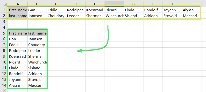
In Excel, you can do this manually or automatically in multiple ways depending on your purpose. Read on to get all the details and choose the best solution for yourself.

How to convert rows into columns or columns to rows in Excel – the basic solution

The easiest way to convert rows to columns in Excel is via the Paste Transpose option. Here is how it looks:

Select and copy the needed range
Right-click on a cell where you want to convert rows to columns
Select the Paste Transpose option to rotate rows to columns

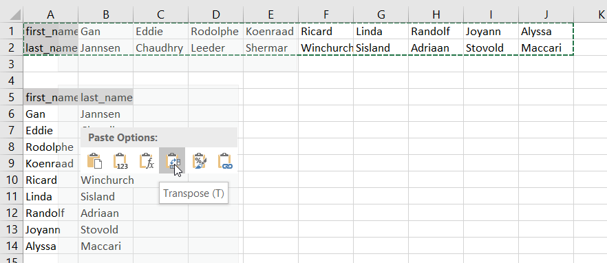
As an alternative, you can use the Paste Special option and mark Transpose using its menu.

It works the same if you need to convert columns to rows in Excel.

This is the best way for a one-time conversion of small to medium numbers of rows both in the Excel desktop and online.

Can I convert multiple rows to columns in Excel from another workbook?

The method above will work well if you want to convert rows to columns in Excel between different workbooks using Excel desktop. You need to have both spreadsheets open and do the copying and pasting as described.

However, in Excel Online, this won’t work for different workbooks. The Paste Transpose option is not available.

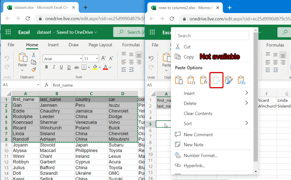
Therefore, in this case, it’s better to use the TRANSPOSE function.

How to switch rows and columns in Excel in more efficient ways

To switch rows and columns in Excel automatically or dynamically, you can use one of these options:

Excel TRANSPOSE function
VBA macro
Power Query

Let’s check out each of them in the example of a data range that we imported to Excel from a Google Sheets file using Coupler.io.

dataset

Coupler.io is an integration solution that synchronizes data between source and destination apps on a regular schedule. For example, you can set up an automatic data export from Google Sheets every day to your Excel workbook.

Check out all the available Excel integrations.

coupler

How to change row to column in Excel with TRANSPOSE

TRANSPOSE is the Excel function that allows you to switch rows and columns in Excel. Here is its syntax:

=TRANSPOSE(array)

array – an array of columns or rows to transpose

One of the main benefits of TRANSPOSE is that it links the converted columns/rows with the source rows/columns. So, if the values in the rows change, the same changes will be made in the converted columns.

TRANSPOSE formula to convert multiple rows to columns in Excel desktop

TRANSPOSE is an array formula, which means that you’ll need to select a number of cells in the columns that correspond to the number of cells in the rows to be converted and press Ctrl+Shift+Enter.

=TRANSPOSE(A1:J2)

Fortunately, you don’t have to go through this procedure in Excel Online.

TRANSPOSE formula to rotate row to column in Excel Online

You can simply insert your TRANSPOSE formula in a cell and hit enter. The rows will be rotated to columns right away without any additional button combinations.

Excel TRANSPOSE multiple rows in a group to columns between different workbooks

We promised to demonstrate how you can use TRANSPOSE to rotate rows to columns between different workbooks. In Excel Online, you need to do the following:

Copy a range of columns to rotate from one spreadsheet and paste it as a link to another spreadsheet.

We need this URL path to use in the TRANSPOSE formula, so copy it.

The URL path above is for a cell, not for an array. So, you’ll need to slightly update it to an array to use in your TRANSPOSE formula. Here is what it should look like:

=TRANSPOSE('https://d.docs.live.net/ec25d9990d879c55/Docs/Convert rows to columns/[dataset.xlsx]dataset'!A1:D12)

You can follow the same logic for rotating rows to columns between workbooks in Excel desktop.

Are there other formulas to convert columns to rows in Excel?

TRANSPOSE is not the only function you can use to change rows to columns in Excel. A combination of INDIRECT and ADDRESS functions can be considered as an alternative, but the flow to convert rows to columns in Excel using this formula is much trickier. Let’s check it out in the following example.

How to convert text in columns to rows in Excel using INDIRECT+ADDRESS

If you have a set of columns with the first cell A1, the following formula will allow you to convert columns to rows in Excel.

=INDIRECT(ADDRESS(COLUMN(A1),ROW(A1)))

But where are the rows, you may ask! Well, first you need to drag this formula down if you are converting multiple columns to rows. Then drag it to the right.

NOTE: This Excel formula only to convert data in columns to rows starting with A1 cell. If your columns start from another cell, check out the next section.

How to convert Excel data in columns to rows using INDIRECT+ADDRESS from other cells

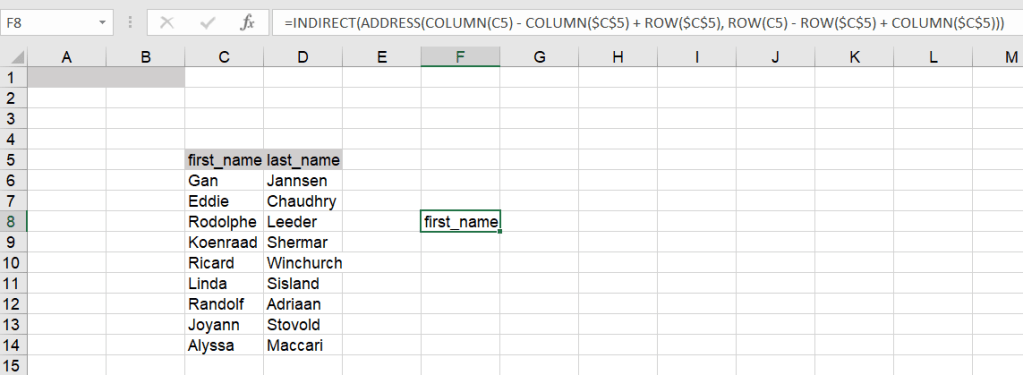
To convert columns to rows in Excel with INDIRECT+ADDRESS formulas from not A1 cell only, use the following formula:

=INDIRECT(ADDRESS(COLUMN(first_cell) - COLUMN($first_cell) + ROW($first_cell), ROW(first_cell) - ROW($first_cell) + COLUMN($first_cell)))

first_cell – enter the first cell of your columns

Here is an example of how to convert Excel data in columns to rows:

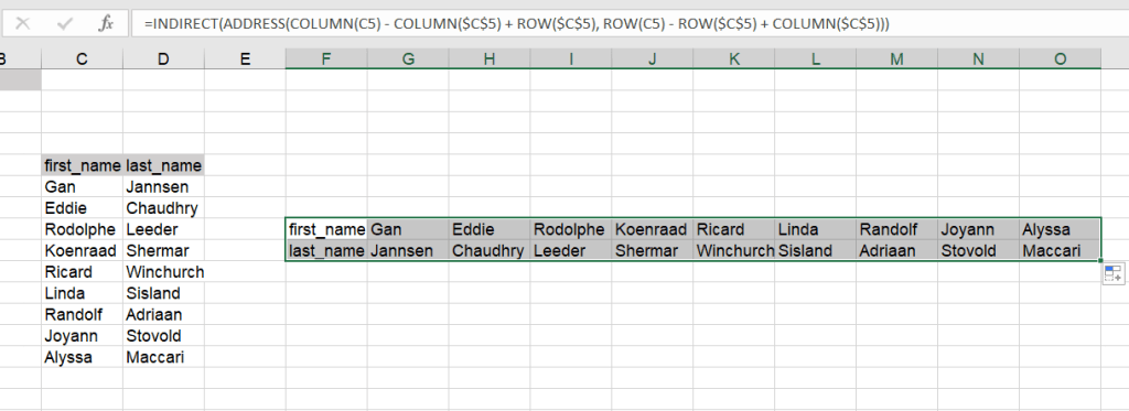
=INDIRECT(ADDRESS(COLUMN(C5) - COLUMN($C$5) + ROW($C$5), ROW(C5) - ROW($C$5) + COLUMN($C$5)))

Again, you’ll need to drag the formula down and to the right to populate the rest of the cells.

How to automatically convert rows to columns in Excel VBA

VBA is a superb option if you want to customize some function or functionality. However, this option is only code-based. Below we provide a script that allows you to change rows to columns in Excel automatically.

Go to the Visual Basic Editor (VBE). Click Alt+F11 or you can go to the Developer tab => Visual Basic.

In VBE, go to Insert => Module.

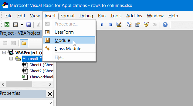
Copy and paste the script into the window. You’ll find the script in the next section.

Now you can close the VBE. Go to Developer => Macros and you’ll see your RowsToColumns macro. Click Run.

You’ll be asked to select the array to rotate and the cell to insert the rotated columns.

There you go!

VBA macro script to convert multiple rows to columns in Excel

Sub TransposeColumnsRows()
    Dim SourceRange As Range
    Dim DestRange As Range
 
    Set SourceRange = Application.InputBox(Prompt:="Please select the range to transpose", Title:="Transpose Rows to Columns", Type:=8)
    Set DestRange = Application.InputBox(Prompt:="Select the upper left cell of the destination range", Title:="Transpose Rows to Columns", Type:=8)
 
    SourceRange.Copy
    DestRange.Select
    Selection.PasteSpecial Paste:=xlPasteAll, Operation:=xlNone, SkipBlanks:=False, Transpose:=True
    Application.CutCopyMode = False
 
End Sub

Sub RowsToColumns()
    Dim SourceRange As Range
    Dim DestRange As Range
 
    Set SourceRange = Application.InputBox(Prompt:="Select the array to rotate", Title:="Convert Rows to Columns", Type:=8)
    Set DestRange = Application.InputBox(Prompt:="Select the cell to insert the rotated columns", Title:="Convert Rows to Columns", Type:=8)
 
    SourceRange.Copy
    DestRange.Select
    Selection.PasteSpecial Paste:=xlPasteAll, Operation:=xlNone, SkipBlanks:=False, Transpose:=True
    Application.CutCopyMode = False
 
End Sub

Read more in our Excel Macros Tutorial.

Convert rows to column in Excel using Power Query

Power Query is another powerful tool available for Excel users. We wrote a separate Power Query Tutorial, so feel free to check it out.

Meanwhile, you can use Power Query to transpose rows to columns. To do this, go to the Data tab, and create a query from table.

Then select a range of cells to convert rows to columns in Excel. Click OK to open the Power Query Editor.

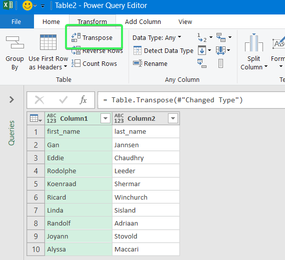
In the Power Query Editor, go to the Transform tab and click Transpose. The rows will be rotated to columns.

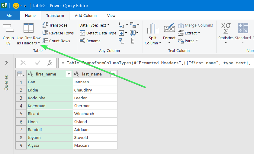
If you want to keep the headers for your columns, click the Use First Row as Headers button.

That’s it. You can Close & Load your dataset – the rows will be converted to columns.

Error message when trying to convert rows to columns in Excel

To wrap up with converting Excel data in columns to rows, let’s review the typical error messages you can face during the flow.

Overlap error

The overlap error occurs when you’re trying to paste the transposed range into the area of the copied range. Please avoid doing this.

Wrong data type error

You may see this #VALUE! error when you implement the TRANSPOSE formula in Excel desktop without pressing Ctrl+Shift+Enter.

Other errors may be caused by typos or other misprints in the formulas you use to convert groups of data from rows to columns in Excel. Always double-check the syntax before pressing Enter or Ctrl+Shift+Enter 🙂 . Good luck with your data!

A content manager at Coupler.io whose key responsibility is to ensure that the readers love our content on the blog. With 5 years of experience as a wordsmith in SaaS, I know how to make texts resonate with readers’ queries✍🏼

Back to Blog

Focus on your business

goals while we take care of your data!

Try Coupler.io

Источник

Sub multiple_columns_to_one()'
' multiple_columns_to_one Macro
'


' This will take all values from Columns B to BZ and stack them into column A.
    Dim K As Long, ar
    K = 1
    For Each ar In Array("B", "C", "D", "E", "F", "G", "H", "I", "J", "K", "L", "M", "N", "O", "P", "Q", "R", "S", "T", "U", "V", "W", "X", "Y", "Z", "AA", "AB", "AC", "AD", "AE", "AF", "AG", "AH", "AI", "AJ", "AK", "AL", "AM", "AN", "AO", "AP", "AQ", "AR", "AS", "AT", "AU", "AV", "AW", "AX", "AY", "AZ", "BA", "BB", "BC", "BD", "BE", "BF", "BG", "BH", "BI", "BJ", "BK", "BL", "BM", "BN", "BO", "BP", "BQ", "BR", "BS", "BT", "BU", "BV", "BW", "BX", "BY", "BZ")
        For i = 1 To 10000
            If Cells(i, ar).Value <> "" Then
                Cells(K, "A").Value = Cells(i, ar).Value
                K = K + 1
            End If
        Next i
    Next ar
End Sub

Источник

Question

Answers

How to convert rows into columns or columns to rows in Excel – the basic solution

Can I convert multiple rows to columns in Excel from another workbook?

How to switch rows and columns in Excel in more efficient ways

How to change row to column in Excel with TRANSPOSE

TRANSPOSE formula to convert multiple rows to columns in Excel desktop

TRANSPOSE formula to rotate row to column in Excel Online

Excel TRANSPOSE multiple rows in a group to columns between different workbooks

Are there other formulas to convert columns to rows in Excel?

How to convert text in columns to rows in Excel using INDIRECT+ADDRESS

How to convert Excel data in columns to rows using INDIRECT+ADDRESS from other cells

How to automatically convert rows to columns in Excel VBA

VBA macro script to convert multiple rows to columns in Excel

Convert rows to column in Excel using Power Query

Error message when trying to convert rows to columns in Excel

Overlap error

Wrong data type error

Focus on your business goals while we take care of your data!

Focus on your business

goals while we take care of your data!