Содержание
- Find and select cells that meet specific conditions
- Need more help?
- Find and select cells that meet specific conditions
- Need more help?
- Highlight Rows Based on a Cell Value in Excel (Conditional Formatting)
- Highlight Rows Based on a Text Criteria
- Highlight Rows Based on a Number Criteria
- Highlight Rows Based on a Multiple Criteria (AND/OR)
- Highlight Rows in Different Color Based on Multiple Conditions
- Highlight Rows Where Any Cell is Blank
- Highlight Rows Based on Drop Down Selection
Find and select cells that meet specific conditions
Use the Go To command to quickly find and select all cells that contain specific types of data, such as formulas. Also, use Go To to find only the cells that meet specific criteria,—such as the last cell on the worksheet that contains data or formatting.
Follow these steps:
Begin by doing either of the following:
To search the entire worksheet for specific cells, click any cell.
To search for specific cells within a defined area, select the range, rows, or columns that you want. For more information, see Select cells, ranges, rows, or columns on a worksheet.
Tip: To cancel a selection of cells, click any cell on the worksheet.
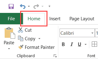
On the Home tab, click Find & Select > Go To (in the Editing group).
Keyboard shortcut: Press CTRL+G.
In the Go To Special dialog box, click one of the following options.
Cells that contain comments.
Cells that contain constants.
Cells that contain formulas.
Note: The check boxes below Formulas define the type of formula.
The current region, such as an entire list.
An entire array if the active cell is contained in an array.
Graphical objects, including charts and buttons, on the worksheet and in text boxes.
All cells that differ from the active cell in a selected row. There is always one active cell in a selection—whether this is a range, row, or column. By pressing the Enter or Tab key, you can change the location of the active cell, which by default is the first cell in a row.
If more than one row is selected, the comparison is done for each individual row of that selection, and the cell that is used in the comparison for each additional row is located in the same column as the active cell.
All cells that differ from the active cell in a selected column. There is always one active cell in a selection, whether this is a range, row, or column. By pressing the Enter or Tab key, you can change the location of the active cell—which by default is the first cell in a column.
When selecting more than one column, the comparison is done for each individual column of that selection. The cell that is used in the comparison for each additional column is located in the same row as the active cell.
Cells that are referenced by the formula in the active cell. Under Dependents, do either of the following:
Click Direct only to find only cells that are directly referenced by formulas.
Click All levels to find all cells that are directly or indirectly referenced by the cells in the selection.
Cells with formulas that refer to the active cell. Do either of the following:
Click Direct only to find only cells with formulas that refer directly to the active cell.
Click All levels to find all cells that directly or indirectly refer to the active cell.
The last cell on the worksheet that contains data or formatting.
Visible cells only
Only cells that are visible in a range that crosses hidden rows or columns.
Only cells that have conditional formats applied. Under Data validation, do either of the following:
Click All to find all cells that have conditional formats applied.
Click Same to find cells that have the same conditional formats as the currently selected cell.
Only cells that have data validation rules applied. Do either of the following:
Click All to find all cells that have data validation applied.
Click Same to find cells that have the same data validation as the currently selected cell.
Need more help?
You can always ask an expert in the Excel Tech Community or get support in the Answers community.
Источник
Find and select cells that meet specific conditions
Use the Go To command to quickly find and select all cells that contain specific types of data, such as formulas. Also, use Go To to find only the cells that meet specific criteria,—such as the last cell on the worksheet that contains data or formatting.
Follow these steps:
Begin by doing either of the following:
To search the entire worksheet for specific cells, click any cell.
To search for specific cells within a defined area, select the range, rows, or columns that you want. For more information, see Select cells, ranges, rows, or columns on a worksheet.
Tip: To cancel a selection of cells, click any cell on the worksheet.
On the Home tab, click Find & Select > Go To (in the Editing group).
Keyboard shortcut: Press CTRL+G.
In the Go To Special dialog box, click one of the following options.
Cells that contain comments.
Cells that contain constants.
Cells that contain formulas.
Note: The check boxes below Formulas define the type of formula.
The current region, such as an entire list.
An entire array if the active cell is contained in an array.
Graphical objects, including charts and buttons, on the worksheet and in text boxes.
All cells that differ from the active cell in a selected row. There is always one active cell in a selection—whether this is a range, row, or column. By pressing the Enter or Tab key, you can change the location of the active cell, which by default is the first cell in a row.
If more than one row is selected, the comparison is done for each individual row of that selection, and the cell that is used in the comparison for each additional row is located in the same column as the active cell.
All cells that differ from the active cell in a selected column. There is always one active cell in a selection, whether this is a range, row, or column. By pressing the Enter or Tab key, you can change the location of the active cell—which by default is the first cell in a column.
When selecting more than one column, the comparison is done for each individual column of that selection. The cell that is used in the comparison for each additional column is located in the same row as the active cell.
Cells that are referenced by the formula in the active cell. Under Dependents, do either of the following:
Click Direct only to find only cells that are directly referenced by formulas.
Click All levels to find all cells that are directly or indirectly referenced by the cells in the selection.
Cells with formulas that refer to the active cell. Do either of the following:
Click Direct only to find only cells with formulas that refer directly to the active cell.
Click All levels to find all cells that directly or indirectly refer to the active cell.
The last cell on the worksheet that contains data or formatting.
Visible cells only
Only cells that are visible in a range that crosses hidden rows or columns.
Only cells that have conditional formats applied. Under Data validation, do either of the following:
Click All to find all cells that have conditional formats applied.
Click Same to find cells that have the same conditional formats as the currently selected cell.
Only cells that have data validation rules applied. Do either of the following:
Click All to find all cells that have data validation applied.
Click Same to find cells that have the same data validation as the currently selected cell.
Need more help?
You can always ask an expert in the Excel Tech Community or get support in the Answers community.
Источник
Highlight Rows Based on a Cell Value in Excel (Conditional Formatting)
Watch Video – Highlight Rows based on Cell Values in Excel
In case you prefer reading written instruction instead, below is the tutorial.
Conditional Formatting allows you to format a cell (or a range of cells) based on the value in it.
But sometimes, instead of just getting the cell highlighted, you may want to highlight the entire row (or column) based on the value in one cell.
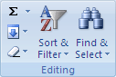
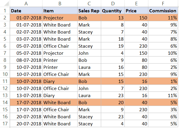
To give you an example, below I have a dataset where I have highlighted all the rows where the name of the Sales Rep is Bob.

In this tutorial, I will show you how to highlight rows based on a cell value using conditional formatting using different criteria.
Click here to download the Example file and follow along.
This Tutorial Covers:
Highlight Rows Based on a Text Criteria
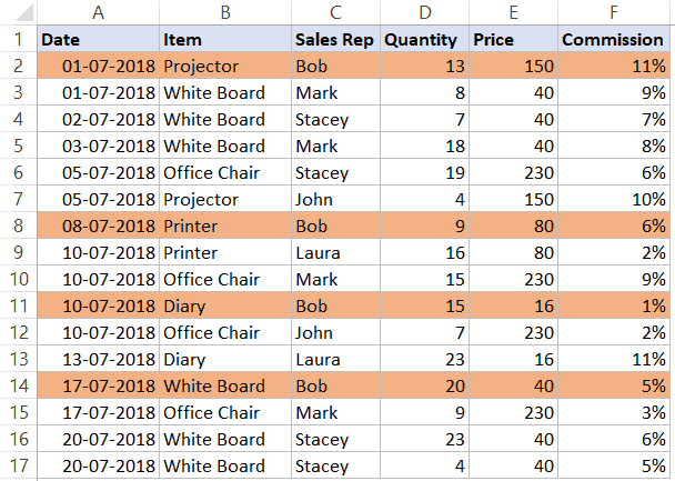
Suppose you have a dataset as shown below and you want to highlight all the records where the Sales Rep name is Bob.
Here are the steps to do this:
- Select the entire dataset (A2:F17 in this example).
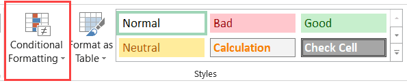
- Click the Home tab.

- In the Styles group, click on Conditional Formatting.
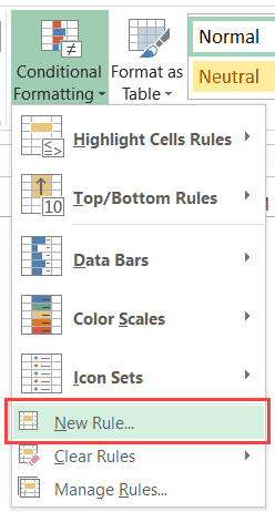
- Click on ‘New Rules’.
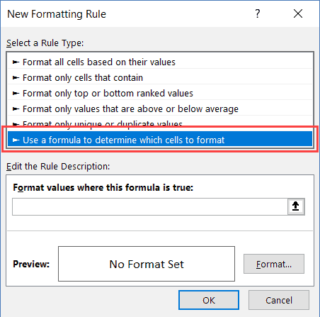
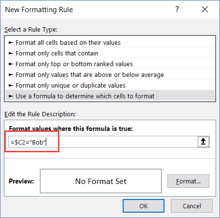
- In the ‘New Formatting Rule’ dialog box, click on ‘Use a formula to determine which cells to format’.
- In the formula field, enter the following formula: =$C2=”Bob”
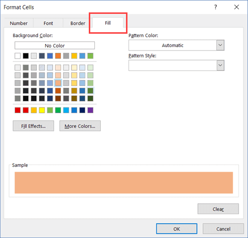
- Click the ‘Format’ button.
- In the dialog box that opens, set the color in which you want the row to get highlighted.
- Click OK.
This will highlight all the rows where the name of the Sales Rep is ‘Bob’.
Click here to download the Example file and follow along.
How does it Work?
Conditional Formatting checks each cell for the condition we have specified, which is =$C2=”Bob”
So when it’s analyzing each cell in row A2, it will check whether the cell C2 has the name Bob or not. If it does, that cell gets highlighted, else it doesn’t.
Note that the trick here is to use a dollar sign ($) before the column alphabet ($C1). By doing this, we have locked the column to always be C. So even when cell A2 is being checked for the formula, it will check C2, and when A3 is checked for the condition, it will check C3.
This allows us to highlight the entire row by conditional formatting.
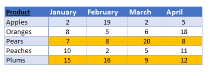
Highlight Rows Based on a Number Criteria
In the above example, we saw how to check for a name and highlight the entire row.
We can use the same method to also check for numeric values and highlight rows based on a condition.
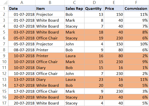
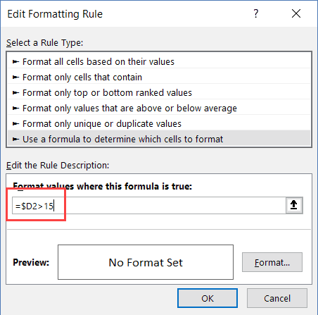
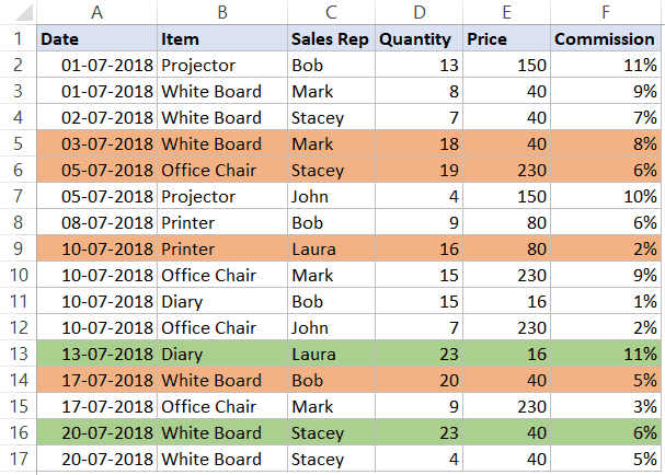
Suppose I have the same data (as shown below), and I want to highlight all the rows where the quantity is more than 15.
Here are the steps to do this:
- Select the entire dataset (A2:F17 in this example).
- Click the Home tab.
- In the Styles group, click on Conditional Formatting.
- Click on ‘New Rules’.
- In the ‘New Formatting Rule’ dialog box, click on ‘Use a formula to determine which cells to format’.
- In the formula field, enter the following formula: =$D2>=15
- Click the ‘Format’ button. In the dialog box that opens, set the color in which you want the row to get highlighted.
- Click OK.
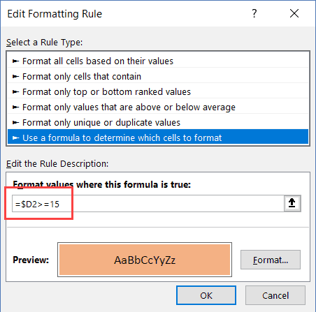
This will highlight all the rows where the quantity is more than or equal to 15.
Similarly, we can also use this to have criteria for the date as well.
For example, if you want to highlight all the rows where the date is after 10 July 2018, you can use the below date formula:
Highlight Rows Based on a Multiple Criteria (AND/OR)
You can also use multiple criteria to highlight rows using conditional formatting.
For example, if you want to highlight all the rows where the Sales Rep name is ‘Bob’ and the quantity is more than 10, you can do that using the following steps:
- Select the entire dataset (A2:F17 in this example).
- Click the Home tab.
- In the Styles group, click on Conditional Formatting.
- Click on ‘New Rules’.
- In the ‘New Formatting Rule’ dialog box, click on ‘Use a formula to determine which cells to format’.
- In the formula field, enter the following formula: =AND($C2=”Bob”,$D2>10)
- Click the ‘Format’ button. In the dialog box that opens, set the color in which you want the row to get highlighted.
- Click OK.
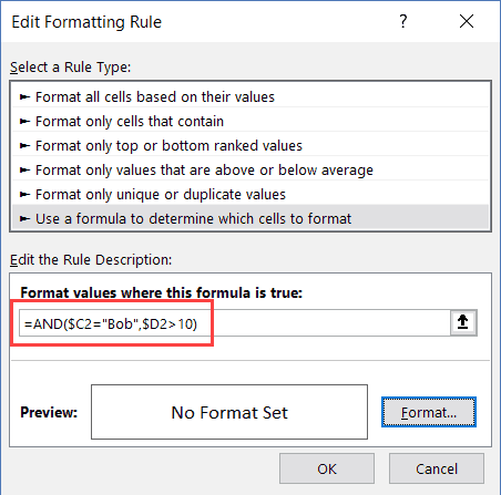
In this example, only those rows get highlighted where both the conditions are met (this is done using the AND formula).
Similarly, you can also use the OR condition. For example, if you want to highlight rows where either the sales rep is Bob or the quantity is more than 15, you can use the below formula:
Click here to download the Example file and follow along.
Highlight Rows in Different Color Based on Multiple Conditions
Sometimes, you may want to highlight rows in a color based on the condition.
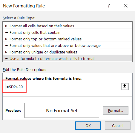
For example, you may want to highlight all the rows where the quantity is more than 20 in green and where the quantity is more than 15 (but less than 20) in orange.
To do this, you need to create two conditional formatting rules and set the priority.
Here are the steps to do this:
- Select the entire dataset (A2:F17 in this example).
- Click the Home tab.
- In the Styles group, click on Conditional Formatting.
- Click on ‘New Rules’.
- In the ‘New Formatting Rule’ dialog box, click on ‘Use a formula to determine which cells to format’.
- In the formula field, enter the following formula: =$D2>15
- Click the ‘Format’ button. In the dialog box that opens, set the color to Orange.
- Click OK.
- In the ‘Conditional Formatting Rules Manager’ dialog box, click on ‘New Rule’.
- In the ‘New Formatting Rule’ dialog box, click on ‘Use a formula to determine which cells to format’.
- In the formula field, enter the following formula: =$D2>20
- Click the ‘Format’ button. In the dialog box that opens, set the color to Green.
- Click OK.
- Click Apply (or OK).
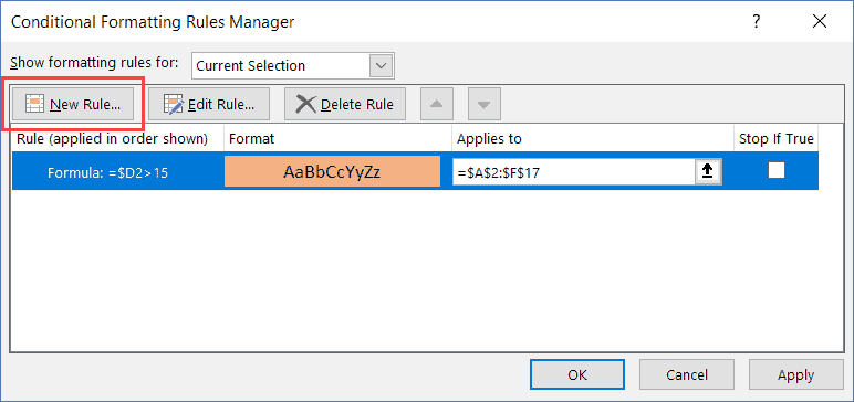
The above steps would make all the rows with quantity more than 20 in green and those with more than 15 (but less than equal to 20 in orange).
Understanding the Order of Rules:
When using multiple conditions, it important to make sure the order of the conditions is correct.
In the above example, the Green color condition is above the Orange color condition.
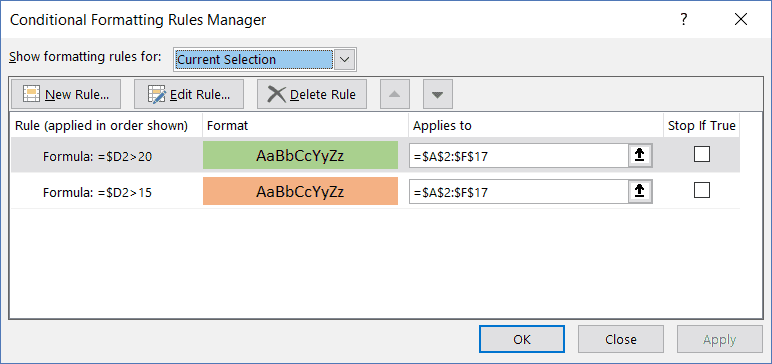
If it’s the other way round, all the rows would be colored in orange only.
Because a row where quantity is more than 20 (say 23) satisfies both our conditions (=$D2>15 and =$D2>20). And since Orange condition is at the top, it gets preference.
You can change the order of the conditions by using the Move Up/Down buttons.
Click here to download the Example file and follow along.
Highlight Rows Where Any Cell is Blank
If you want to highlight all rows where any of the cells in it is blank, you need to check for each cell using conditional formatting.
Here are the steps to do this:
- Select the entire dataset (A2:F17 in this example).
- Click the Home tab.
- In the Styles group, click on Conditional Formatting.
- Click on ‘New Rules’.
- In the ‘New Formatting Rule’ dialog box, click on ‘Use a formula to determine which cells to format’.
- In the formula field, enter the following formula: =COUNTIF($A2:$F2,””)>0
- Click the ‘Format’ button. In the dialog box that opens, set the color to Orange.
- Click OK.
The above formula counts the number of blank cells. If the result is more than 0, it means there are blank cells in that row.
If any of the cells are empty, it highlights the entire row.
![]()
Related: Read this tutorial if you only want to highlight the blank cells.
Highlight Rows Based on Drop Down Selection
In the examples covered so far, all the conditions were specified with the conditional formatting dialog box.
In this part of the tutorial, I will show you how to make it dynamic (so that you can enter the condition within a cell in Excel and it will automatically highlight the rows based on it).
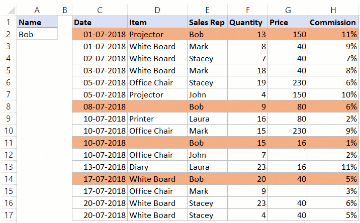
Below is an example, where I select a name from the drop-down, and all the rows with that name get highlighted:
Here are the steps to create this:
- Create a drop-down list in cell A2. Here I have used the names of the sales rep to create the drop down list. Here is a detailed guide on how to create a drop-down list in Excel.
- Select the entire dataset (C2:H17 in this example).
- Click the Home tab.
- In the Styles group, click on Conditional Formatting.
- Click on ‘New Rules’.
- In the ‘New Formatting Rule’ dialog box, click on ‘Use a formula to determine which cells to format’.
- In the formula field, enter the following formula: =$E2=$A$2
- Click the ‘Format’ button. In the dialog box that opens, set the color to Orange.
- Click OK.
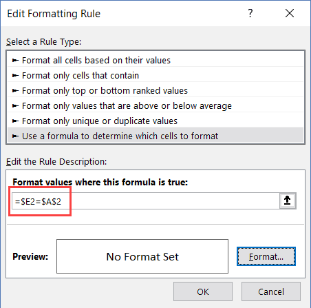
Now when you select any name from the drop-down, it will automatically highlight the rows where the name is the same that you have selected from the drop-down.
Interested in learning more on how to search and highlight in Excel? Check the below videos.
You May Also Like the Following Excel Tutorials:
Источник
Excel for Microsoft 365 Excel 2021 Excel 2019 Excel 2016 Excel 2013 Excel 2010 Excel 2007 Access 2007 More…Less
Use the Go To command to quickly find and select all cells that contain specific types of data, such as formulas. Also, use Go To to find only the cells that meet specific criteria,—such as the last cell on the worksheet that contains data or formatting.
Follow these steps:
-
Begin by doing either of the following:
-
To search the entire worksheet for specific cells, click any cell.
-
To search for specific cells within a defined area, select the range, rows, or columns that you want. For more information, see Select cells, ranges, rows, or columns on a worksheet.
Tip: To cancel a selection of cells, click any cell on the worksheet.
-
-
On the Home tab, click Find & Select > Go To (in the Editing group).
Keyboard shortcut: Press CTRL+G.
-
Click Special.
-
In the Go To Special dialog box, click one of the following options.
|
Click |
To select |
|---|---|
|
Comments |
Cells that contain comments. |
|
Constants |
Cells that contain constants. |
|
Formulas |
Cells that contain formulas. Note: The check boxes below Formulas define the type of formula. |
|
Blanks |
Blank cells. |
|
Current region |
The current region, such as an entire list. |
|
Current array |
An entire array if the active cell is contained in an array. |
|
Objects |
Graphical objects, including charts and buttons, on the worksheet and in text boxes. |
|
Row differences |
All cells that differ from the active cell in a selected row. There is always one active cell in a selection—whether this is a range, row, or column. By pressing the Enter or Tab key, you can change the location of the active cell, which by default is the first cell in a row. If more than one row is selected, the comparison is done for each individual row of that selection, and the cell that is used in the comparison for each additional row is located in the same column as the active cell. |
|
Column differences |
All cells that differ from the active cell in a selected column. There is always one active cell in a selection, whether this is a range, row, or column. By pressing the Enter or Tab key, you can change the location of the active cell—which by default is the first cell in a column. When selecting more than one column, the comparison is done for each individual column of that selection. The cell that is used in the comparison for each additional column is located in the same row as the active cell. |
|
Precedents |
Cells that are referenced by the formula in the active cell. Under Dependents, do either of the following:
|
|
Dependents |
Cells with formulas that refer to the active cell. Do either of the following:
|
|
Last cell |
The last cell on the worksheet that contains data or formatting. |
|
Visible cells only |
Only cells that are visible in a range that crosses hidden rows or columns. |
|
Conditional formats |
Only cells that have conditional formats applied. Under Data validation, do either of the following:
|
|
Data validation |
Only cells that have data validation rules applied. Do either of the following:
|
Need more help?
You can always ask an expert in the Excel Tech Community or get support in the Answers community.
Need more help?
Want more options?
Explore subscription benefits, browse training courses, learn how to secure your device, and more.
Communities help you ask and answer questions, give feedback, and hear from experts with rich knowledge.
Author: Oscar Cronquist Article last updated on March 06, 2023
I will in this article demonstrate several techniques that extract or filter records based on two conditions applied to a single column in your dataset. For example, if you use the array formula then the result will refresh instantly when you enter new start and end values.
The remaining built-in techniques need a little more manual work in order to apply new conditions, however, they are fast. The downside with the array formula is that it may become slow if you are working with huge amounts of data.
I have also written an article in case you need to find records that match one condition in one column and another condition in another column. The following article shows you how to build a formula that uses an arbitrary number of conditions: Extract records where all criteria match if not empty
This article Extract records between two dates is very similar to the current one you are reading right now, Excel dates are actually numbers formatted as dates in Excel. If you want to search for a text string within a given date range then read this article: Filter records based on a date range and a text string
I must recommend this article if you want to do a wildcard search across all columns in a data set, it also returns all matching records. If you want to extract records based on criteria and not a numerical range then read this part of this article.
What is on this page?
- Extract all rows from a range based on range criteria (Array formula)
- Video
- How to enter an array formula
- Explaining array formula
- Extract all rows from a range based on range criteria — Excel 365
- Explaining formula
- Extract all rows from a range based on multiple conditions (Array formula)
- Explaining array formula
- Extract all rows from a range based on multiple conditions — Excel 365
- Explaining formula
- Extract all rows from a range based on range critera
[Excel defined Table] - Extract all rows from a range based on range critera
[AutoFilter] - Extract all rows from a range based on range criteria
[Advanced Filter] - Get Excel file
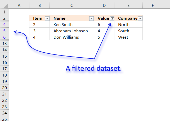
1. Extract all rows from a range based on range criteria
[Array formula]
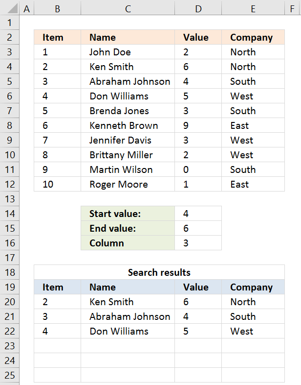
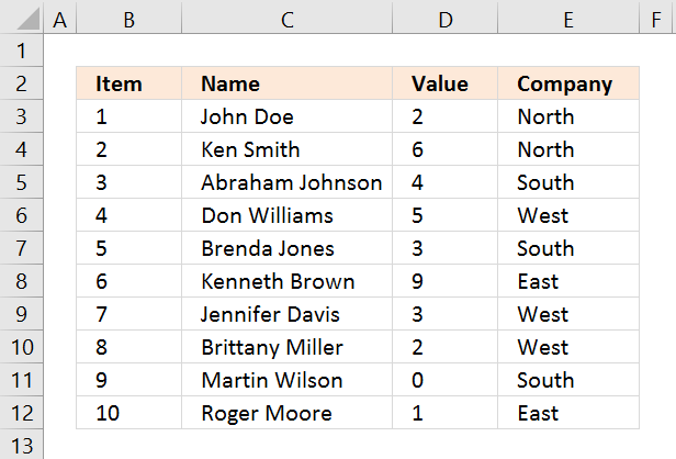
The picture above shows you a dataset in cell range B3:E12, the search parameters are in D14:D16. The search results are in B20:E22.
Cells D14 allows you to specify the start number, and cell D15 is the end number of the range. Cell D16 determines which column to use in cell range B3:E12.
The result is presented in cells B20:E20 and cells below. The example above shows a start value of 4 and an end value of 6, the column is three meaning the third column in cell range B3:E12.
All records that match range 4 to 6 in cell range D3:D12 are extracted, D3:D12 is the third column in B3:E12.
Update 20 Sep 2017, a smaller formula in cell A20.
Array formula in cell A20:
=INDEX($B$3:$E$12, SMALL(IF((INDEX($B$3:$E$12, , $D$16)< =$D$15)*(INDEX($B$3:$E$12, , $D$16)> =$D$14), MATCH(ROW($B$3:$E$12), ROW($B$3:$E$12)), «»), ROWS(B20:$B$20)), COLUMNS($A$1:A1))
Back to top
1.1 Video
See this video to learn more about the formula:
Back to top
1.2 How to enter this array formula
- Select cell A20
- Paste above formula to cell or formula bar
- Press and hold CTRL + SHIFT simultaneously
- Press Enter once
- Release all keys
The formula bar now shows the formula with a beginning and ending curly bracket, that is if you did the above steps correctly. Like this:
{=array_formula}
Don’t enter these characters yourself, they appear automatically.
Now copy cell A20 and paste to cell range A20:E22.
Back to top
1.3 Explaining array formula in cell A20
You can follow along if you select cell A19, go to tab «Formulas» on the ribbon and press with left mouse button on the «Evaluate Formula» button.
Step 1 — Filter a specific column in cell range B3:E12
The INDEX function is mostly used for getting a single value from a given cell range, however, it can also return an entire column or row from a cell range.
This is exactly what I am doing here, the column number specified in cell D16 determines which column to extract.
INDEX($B$3:$E$12, , $D$16, 1)
becomes
INDEX($B$3:$E$12, , 3, 1)
and returns C3:C12.
Recommended articles
Step 2 — Check which values are smaller or equal to the condition
The smaller than and equal sign are logical operators that let you compare value to value, in this case, if a number is smaller than or equal to another number.
The output is a boolean value, True och False. Their positions in the array correspond to the positions in the cell range.
INDEX($B$3:$E$12, , $D$16, 1)< =$D$15
becomes
C3:C12< =$D$15
becomes
{2; 6; 4; 5; 3; 9; 3; 2; 0; 1}<=6
and returns
{TRUE; TRUE; TRUE; TRUE; TRUE; FALSE; TRUE; TRUE; TRUE; TRUE}.
Step 3 — Multiply arrays — AND logic
There is a second condition we need to evaluate before we know which records are in range.
(INDEX($B$3:$E$12, , $D$16, 1)< =$D$15)*(INDEX($B$3:$E$12, , $D$16, 1)> =$D$14)
becomes
({2; 6; 4; 5; 3; 9; 3; 2; 0; 1}< =$C$14)*({2; 6; 4; 5; 3; 9; 3; 2; 0; 1}> =$C$13)
becomes
({2; 6; 4; 5; 3; 9; 3; 2; 0; 1}< =3)*({2; 6; 4; 5; 3; 9; 3; 2; 0; 1}> =0)
becomes
{TRUE; FALSE; FALSE; FALSE; TRUE; FALSE; TRUE; TRUE; TRUE; TRUE}*{TRUE; TRUE; TRUE; TRUE; TRUE; TRUE; TRUE; TRUE; TRUE; TRUE}
Both conditions must be met, the asterisk lets us multiple the arrays meaning AND logic.
TRUE * TRUE equals FALSE, all other combinations return False. TRUE * FALSE equals FALSE and so on.
{TRUE; FALSE; FALSE; FALSE; TRUE; FALSE; TRUE; TRUE; TRUE; TRUE} * {TRUE; TRUE; TRUE; TRUE; TRUE; TRUE; TRUE; TRUE; TRUE; TRUE}
returns
{1; 0; 0; 0; 1; 0; 1; 1; 1; 1}.
Boolean values have numerical equivalents, TRUE = 1 and FALSE equals 0 (zero). They are converted when you perform an arithmetic operation in a formula.
Step 4 — Create number sequence
The ROW function calculates the row number of a cell reference.
ROW(reference)
ROW($B$3:$E$12)
returns
{3; 4; 5; 6; 7; 8; 9; 10; 11; 12}.
Step 5 — Create a number sequence from 1 to n
The MATCH function returns the relative position of an item in an array or cell reference that matches a specified value in a specific order.
MATCH(ROW($B$3:$E$12), ROW($B$3:$E$12))
becomes
MATCH({3; 4; 5; 6; 7; 8; 9; 10; 11; 12}, {3; 4; 5; 6; 7; 8; 9; 10; 11; 12})
and returns
{1; 2; 3; 4; 5; 6; 7; 8; 9; 10}.
Step 6 — Return the corresponding row number
The IF function returns one value if the logical test is TRUE and another value if the logical test is FALSE.
IF(logical_test, [value_if_true], [value_if_false])
IF((INDEX($B$3:$E$12, , $D$16)< =$D$15)*(INDEX($B$3:$E$12, , $D$16)> =$D$14), MATCH(ROW($B$3:$E$12), ROW($B$3:$E$12)), «»)
becomes
IF({1; 0; 0; 0; 1; 0; 1; 1; 1; 1}, MATCH(ROW($B$3:$E$12), ROW($B$3:$E$12)), «»)
becomes
IF({1; 0; 0; 0; 1; 0; 1; 1; 1; 1}, {1; 2; 3; 4; 5; 6; 7; 8; 9; 10}, «»)
and returns
{1; «»; «»; «»; 5; «»; 7; 8; 9; 10}.
Step 7 — Extract k-th smallest row number
The SMALL function returns the k-th smallest value from a group of numbers.
SMALL(array, k)
SMALL(IF((INDEX($B$3:$E$12, , $D$16)< =$D$15)*(INDEX($B$3:$E$12, , $D$16)> =$D$14), MATCH(ROW($B$3:$E$12), ROW($B$3:$E$12)), «»), ROWS(B20:$B$20))
becomes
SMALL({1; «»; «»; «»; 5; «»; 7; 8; 9; 10}, ROWS(B20:$B$20))
becomes
SMALL({1; «»; «»; «»; 5; «»; 7; 8; 9; 10}, 1)
and returns 1.
Step 8 — Return the entire row record from the cell range
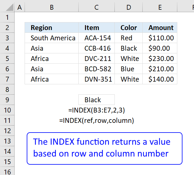
The INDEX function returns a value from a cell range, you specify which value based on a row and column number.
INDEX(array, [row_num], [column_num])
INDEX($B$3:$E$12, SMALL(IF((INDEX($B$3:$E$12, , $D$16)< =$D$15)*(INDEX($B$3:$E$12, , $D$16)> =$D$14), MATCH(ROW($B$3:$E$12), ROW($B$3:$E$12)), «»), ROWS(B20:$B$20)), COLUMNS($A$1:A1))
becomes
INDEX($B$3:$E$12, 1, , 1)
and returns {2, «Ken Smith», 6, «North»}.
Back to top
Recommended articles
Back to top
2. Extract all rows from a range based on range criteria — Excel 365
Update 17 December 2020, the new FILTER function is now available for Excel 365 users.
Excel 365 dynamic array formula in cell B20:
=FILTER($B$3:$E$12, (D3:D12<=D15)*(D3:D12>=D14))
It is a regular formula, however, it returns an array of values and extends automatically to cells below and to the right. Microsoft calls this a dynamic array and spilled array.
The array formula below is for earlier Excel versions, it searches for values that meet a range criterion (cell D14 and D15), the formula lets you change the column to search in with cell D16.
This formula can be used with whatever dataset size and shape. To search the first column, type 1 in cell D16. This is a great improvement in both formula size and how easy it is to enter the formula, compared to the array formula in section 1.
Back to top
2.1 Explaining array formula
Step 1 — First condition
The less than character and the equal sign are both logical operators meaning they are able to compare value to value, the output is a boolean value.
In this case, the logical expression evaluates if numbers in D3:D12 are smaller than or equal to the condition specified in cell D15.
D3:D12<=D15
becomes
{2;6;4;5;3;9;3;2;0;1}<=6
and returns
{TRUE; TRUE; TRUE; TRUE; TRUE; FALSE; TRUE; TRUE; TRUE; TRUE}.
Step 2 — Second condition
The second condition checks if the number in D3:D12 are larger than or equal to the condition specified in cell D14.
D3:D12>=D14
becomes
{2;6;4;5;3;9;3;2;0;1}>=4
and returns
{FALSE; TRUE; TRUE; TRUE; FALSE; TRUE; FALSE; FALSE; FALSE; FALSE}.
Step 3 — Multiply arrays — AND logic
The asterisk lets you multiply a number to a number, in this case, array to array. Both arrays must be of the exact same size.
The parentheses let you control the order of operation, we want to evaluate the comparisons first before we multiply the arrays.
(D3:D12<=D15)*(D3:D12>=D14)
becomes
{TRUE; TRUE; TRUE; TRUE; TRUE; FALSE; TRUE; TRUE; TRUE; TRUE}*{FALSE; TRUE; TRUE; TRUE; FALSE; TRUE; FALSE; FALSE; FALSE; FALSE}
and returns
{0; 1; 1; 1; 0; 0; 0; 0; 0; 0}.
AND logic works like this:
TRUE * TRUE = TRUE (1)
TRUE * FALSE = FALSE (0)
FALSE * TRUE = FALSE (0)
FALSE * FALSE = FALSE (0)
Note that multiplying boolean values returns their numerical equivalents.
TRUE = 1 and FALSE = 0 (zero).
Step 4 — Filter values based on the array
The FILTER function lets you extract values/rows based on a condition or criteria.
FILTER(array, include, [if_empty])
FILTER($B$3:$E$12, (D3:D12<=D15)*(D3:D12>=D14))
becomes
FILTER({1, «John Doe», 2, «North»; 2, «Ken Smith», 6, «North»; 3, «Abraham Johnson», 4, «South»; 4, «Don Williams», 5, «West»; 5, «Brenda Jones», 3, «South»; 6, «Kenneth Brown», 9, «East»; 7, «Jennifer Davis», 3, «West»; 8, «Brittany Miller», 2, «West»; 9, «Martin Wilson», 0, «South»; 10, «Roger Moore», 1, «East»}, (D3:D12<=D15)*(D3:D12>=D14))
becomes
FILTER({1, «John Doe», 2, «North»; 2, «Ken Smith», 6, «North»; 3, «Abraham Johnson», 4, «South»; 4, «Don Williams», 5, «West»; 5, «Brenda Jones», 3, «South»; 6, «Kenneth Brown», 9, «East»; 7, «Jennifer Davis», 3, «West»; 8, «Brittany Miller», 2, «West»; 9, «Martin Wilson», 0, «South»; 10, «Roger Moore», 1, «East»}, {0; 1; 1; 1; 0; 0; 0; 0; 0; 0})
and returns
{2, «Ken Smith», 6, «North»; 3, «Abraham Johnson», 4, «South»; 4, «Don Williams», 5, «West»}.
Back to top
3. Extract all rows from a range that meet the criteria in one column [Array formula]
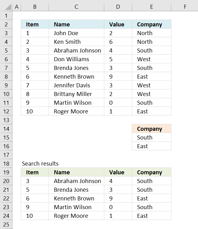
The array formula in cell B20 extracts records where column E equals either «South» or «East». You can use as many conditions as you like as long as you adjust the cell reference $E$15:$E$16 accordingly in the formula below.
The following array formula in cell B20 is for earlier Excel versions than Excel 365:
=INDEX($B$3:$E$12, SMALL(IF(COUNTIF($E$15:$E$16,$E$3:$E$12), MATCH(ROW($B$3:$E$12), ROW($B$3:$E$12)), «»), ROWS(B20:$B$20)), COLUMNS($B$2:B2))
To enter an array formula, type the formula in a cell then press and hold CTRL + SHIFT simultaneously, now press Enter once. Release all keys.
The formula bar now shows the formula with a beginning and ending curly bracket telling you that you entered the formula successfully. Don’t enter the curly brackets yourself.
Back to top
3.1 Explaining formula in cell B20
Step 1 — Filter a specific column in cell range $A$2:$D$11
The COUNTIF function allows you to identify cells in range $E$3:$E$12 that equals $E$15:$E$16.
COUNTIF($E$15:$E$16,$E$3:$E$12)
becomes
COUNTIF({«South»; «East»},{«North»; «North»; «South»; «West»; «South»; «East»; «West»; «West»; «South»; «East»})
and returns
{0;0;1;0;1;1;0;0;1;1}.
Step 2 — Return corresponding row number
The IF function has three arguments, the first one must be a logical expression. If the expression evaluates to TRUE then one thing happens (argument 2) and if FALSE another thing happens (argument 3).
The logical expression was calculated in step 1 , TRUE equals 1 and FALSE equals 0 (zero).
IF(COUNTIF($E$15:$E$16,$E$3:$E$12), MATCH(ROW($B$3:$E$12), ROW($B$3:$E$12)), «»)
becomes
IF({0; 0; 1; 0; 1; 1; 0; 0; 1; 1}, MATCH(ROW($B$3:$E$12), ROW($B$3:$E$12)), «»)
becomes
IF({0; 0; 1; 0; 1; 1; 0; 0; 1; 1}, {1; 2; 3; 4; 5; 6; 7; 8; 9; 10}, «»)
and returns
{«»; «»; 3; «»; 5; 6; «»; «»; 9; 10}.
Step 3 — Find k-th smallest row number
SMALL(IF(COUNTIF($E$15:$E$16,$E$3:$E$12), MATCH(ROW($B$3:$E$12), ROW($B$3:$E$12)), «»), ROWS(B20:$B$20))
becomes
SMALL({«»; «»; 3; «»; 5; 6; «»; «»; 9; 10}, ROWS(B20:$B$20))
becomes
SMALL({«»; «»; 3; «»; 5; 6; «»; «»; 9; 10}, 1)
and returns 3.
Step 4 — Return value based on row and column number
The INDEX function returns a value based on a cell reference and column/row numbers.
INDEX($B$3:$E$12, SMALL(IF(COUNTIF($E$15:$E$16,$E$3:$E$12), MATCH(ROW($B$3:$E$12), ROW($B$3:$E$12)), «»), ROWS(B20:$B$20)), COLUMNS($B$2:B2))
becomes
INDEX($B$3:$E$12, 3, COLUMNS($B$2:B2))
becomes
INDEX($B$3:$E$12, 3, 1)
and returns 3 in cell B20.
Back to top
Recommended articles
Back to top
4. Extract all rows from a range based on multiple conditions — Excel 365
Update 17 December 2020, the new FILTER function is now available for Excel 365 users.
Excel 365 dynamic array formula in cell B20:
=FILTER($B$3:$E$12, COUNTIF(E15:E16, E3:E12))
It is a regular formula, however, it returns an array of values. Read here how it works: Filter values based on criteria
The formula extends automatically to cells below and to the right. Microsoft calls this a dynamic array and spilled array.
Back to top
4.1 Explaining array formula
Step 1 — Check if values equal criteria
The COUNTIF function calculates the number of cells that meet a given condition.
COUNTIF(range, criteria)
COUNTIF($E$15:$E$16,$E$3:$E$12)
becomes
COUNTIF({«South»; «East»},{«North»; «North»; «South»; «West»; «South»; «East»; «West»; «West»; «South»; «East»})
and returns
{0; 0; 1; 0; 1; 1; 0; 0; 1; 1}.
Step 2 — Filter records based on array
The FILTER function lets you extract values/rows based on a condition or criteria.
FILTER(array, include, [if_empty])
FILTER($B$3:$E$12, COUNTIF(E15:E16, E3:E12))
becomes
FILTER($B$3:$E$12, {0; 0; 1; 0; 1; 1; 0; 0; 1; 1})
and returns
{3, «Abraham Johnson», 4, «South»; 5, «Brenda Jones», 3, «South»; 6, «Kenneth Brown», 9, «East»; 9, «Martin Wilson», 0, «South»; 10, «Roger Moore», 1, «East»}.
Back to top
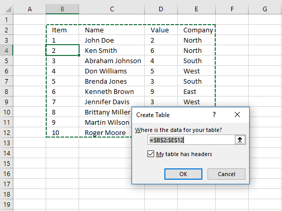
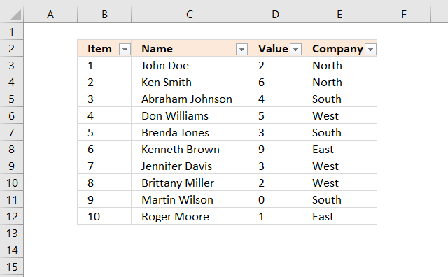
5. Extract all rows from a range that meet the criteria in one column [Excel defined Table]
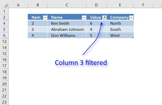
The image above shows a dataset converted to an Excel defined Table, a number filter has been applied to the third column in the table.
Here are the instructions to create an Excel Table and filter values in column 3.
- Select a cell in the dataset.
- Press CTRL + T

- Press with left mouse button on check box «My table has headers».
- Press with left mouse button on OK button.

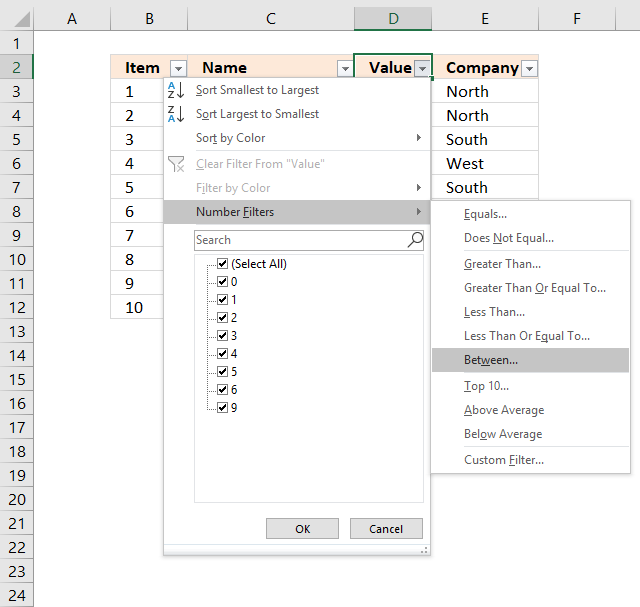
The image above shows the Excel defined Table, here is how to filter D between 4 and 6:
- Press with left mouse button on black arrow next to header.
- Press with left mouse button on «Number Filters».
- Press with left mouse button on «Between…».

- Type 4 and 6.

- Press with left mouse button on OK button.

Back to top
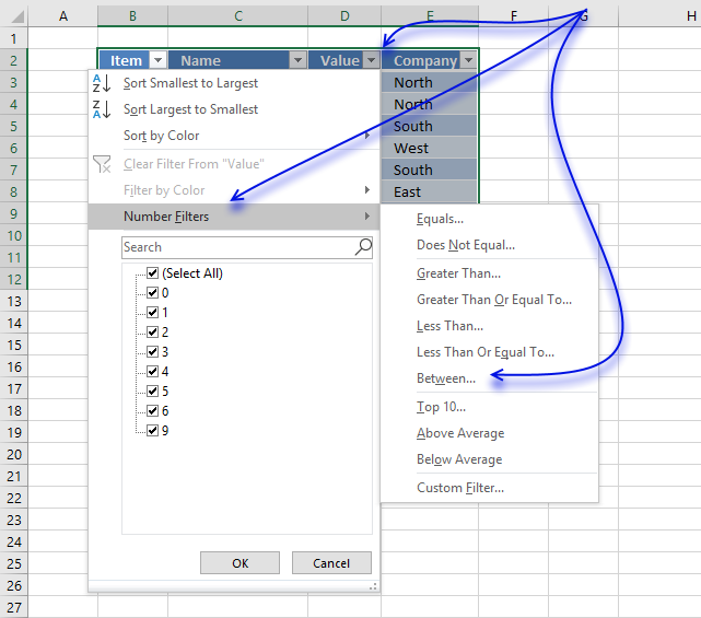
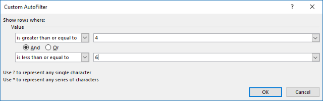
6. Extract all rows from a range that meet the criteria in one column [AutoFilter]
The image above shows filtered records based on two conditions, values in column D are larger or equal to 4 or smaller or equal to 6.
Here is how to apply Filter arrows to a dataset.
- Select any cell within the dataset range.
- Go to tab «Data» on the ribbon.
- Press with left mouse button on «Filter button».

Black arrows appear next to each header.
Lets filter records based on conditions applied to column D.
- Press with left mouse button on the black arrow next to the header in Column D, see the image below.
- Press with left mouse button on «Number Filters».
- Press with left mouse button on «Between».

- Type 4 and 6 in the dialog box shown below.
- Press with left mouse button on OK button.
Back to top
7. Extract all rows from a range that meet the criteria in one column
[Advanced Filter]
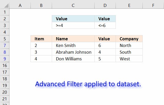
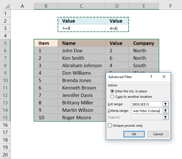
The image above shows a filtered dataset in cell range B5:E15 using Advanced Filter which is a powerful feature in Excel.
Here is how to apply a filter:
- Create headers for the column you want to filter, preferably above or below your data set.
Your filters will possibly disappear if placed next to the data set because rows may become hidden when the filter is applied. - Select the entire dataset including headers.
- Go to tab «Data» on the ribbon.
- Press with left mouse button on the «Advanced» button.

- A dialog box appears.

- Select the criteria range C2:D3, shown ithe n above image.
- Press with left mouse button on OK button.
Back to top
Recommended articles
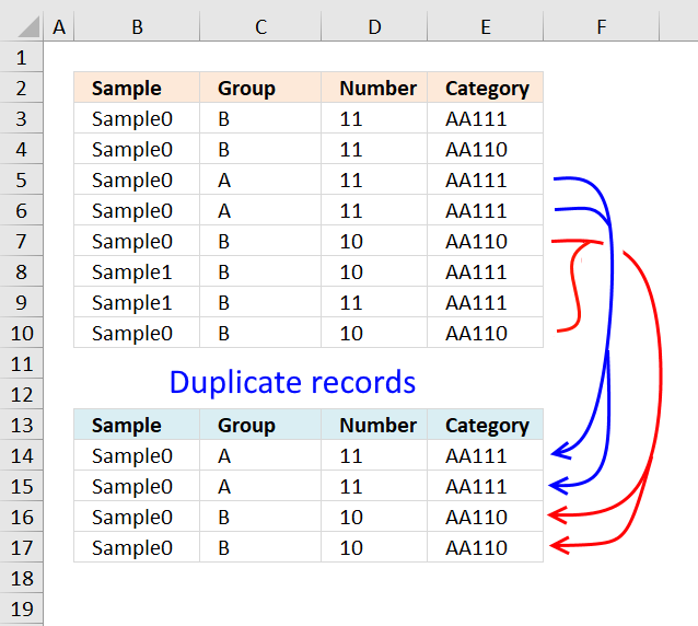
Extract duplicate records
This article describes how to filter duplicate rows with the use of a formula. It is, in fact, an array […]
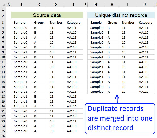
Filter unique distinct records
Table of contents Filter unique distinct row records Filter unique distinct row records but not blanks Filter unique distinct row […]
Back to top
8. Excel file
Back to top
If you work with a large table and you need to search for unique values in Excel that corresponding to a specific request, then you need to use the filter. But sometimes we need to select all the lines that contain to certain values in relation to other lines. In this case, you should use the conditional formatting, which refers to the values of the cells with the query. To get the most effective result, we will use the drop-down list as a query. This is very convenient if you need to frequently change the same type of query to expose of the different table`s rows. We`ll look detailed below: how to make the selection of duplicate cells from the drop-down list.
Selection of the unique and duplicate values in Excel
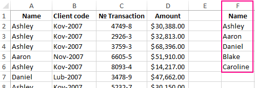
For example, we take the history of mutual settlements with counterparties, as shown in the picture:
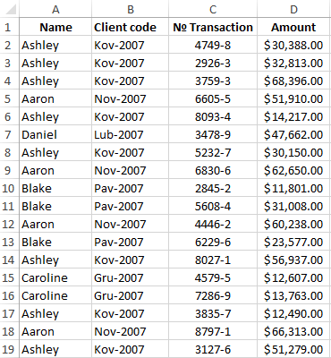
In this table, we need to highlight in color to all transactions for a particular customer. To switch between clients, we will use the drop-down list. Therefore, in the first place, you need to prepare the content for the drop-down list. We need all the customer names from the column A, without repetitions.
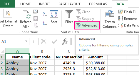
Before selecting to the unique values in Excel, we need to prepare the data for the drop-down list:
- Select to the first column of the table A1:A19.
- Select to the tool: «DATA»-«Sort and Filter»-«Advanced».
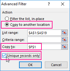
- In the «Advanced Filter» window that appears, you need to turn on «Copy the result to another location», and in the field «Place the result in the range:» to specify $F$1.
- Tick by the check mark to the item «Unique records only» and click OK.
As a result, we got the list of the data with unique values (names without repetitions).
Now we need to slightly modify to our original table. To scroll the first 2 lines and select to the tool: «HOME»-«Cells»-«Insert» or to press the combination of the hot keys CTRL + SHIFT + =.
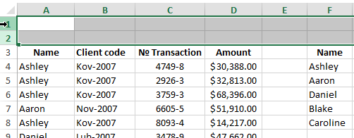
We have added 2 blank lines. Now we enter in the cell A1 to the value «Client:».
It’s time for creating to the drop-down list, from which we will select customer`s names as the query.
Before you select to the unique values from the list, you need to do the following:
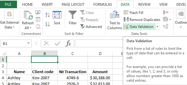
- In the cell B1 you need to select the «DATA»-«Data tool»-«Data Validation».
- On the «Settings» tab in the «Validation criteria» section, from the drop-down list «Allow:», you need to select «List» value.
- In the «Source:» entry field, to put =$F$4:$F$8 and click OK.
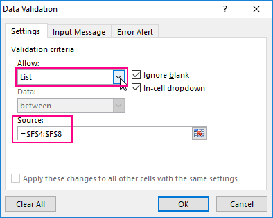
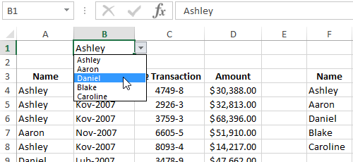
As a result, in the cell B1 we have created the drop-down list of customers` names.
Note. If the data for the drop-down list is in another sheet, then it is better to assign a name for this range and specify it in the «Source:» field. In this case this is not necessary, because all of these data is on the same worksheet.
The selection of the cells from the table by condition in Excel:
- Highlight the tabular part of the original settlement table A4:D21 and select the tool: «HOME»-«Styles»-«Conditional Formatting»-«New Rule»-«Use the formula to define of the formatted cells».
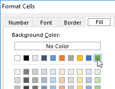
- To select unique values from the column you need to enter the formula: =$A4=$B$1 in the input field and click on the «Format» button to highlight the same cells by color. For example, it will be green color. And to click OK in all are opened windows.
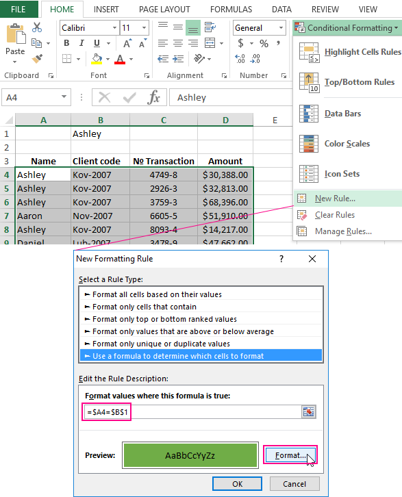
It is done!
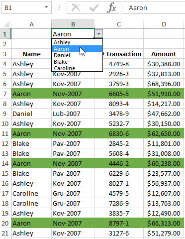
How does work the selection of unique Excel values? When choosing of any value (a name) from the drop-down list B1, all rows that contain this value (name) are highlighted by color in the table. To make sure of this, in the drop-down list B1 you need to choose to a different name. After that, other lines will be automatically highlighted by color. Such table is easy to read and analyze now.
Download example selection from list with conditional formatting.
The principle of automatic highlighting of lines by the query criterion is very simple. Each value in the column A is compared with the value in cell B1. This allows you to find unique values in the Excel table. If the data is the same, then the formula returns to the meaning TRUE and for the whole line is automatically assigned to the new format. In order for the format to be assigned to the entire line, and not just for the cell in column A, we use the mixed reference in the formula =$A4.
This tutorial will demonstrate how to highlight rows if a condition in a cell is met using Conditional Formatting in Excel and Google Sheets.
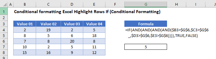
Highlight Rows With Conditional Formatting
IF Function
To highlight a row depending on the value contained in a cell in the row with conditional formatting, you can use the IF Function within a Conditional Formatting rule.
- Select the range you want to apply formatting to.
- In the Ribbon, select Home > Conditional Formatting > New Rule.
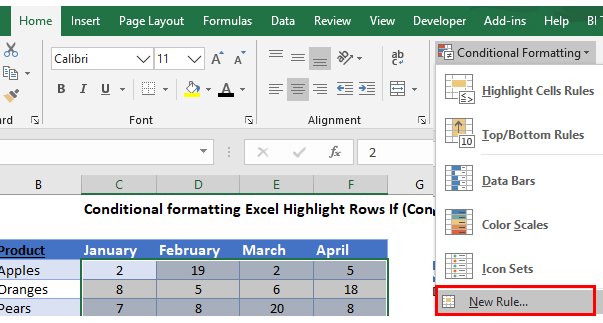
- Select Use a formula to determine which cells to format, and enter the following formula (with the AND Function):
=IF(AND(AND(AND(AND($C3>$H$6,$D3>$H$6,$E3>$H$6, ,$F3>$H$6)))),TRUE,FALSE)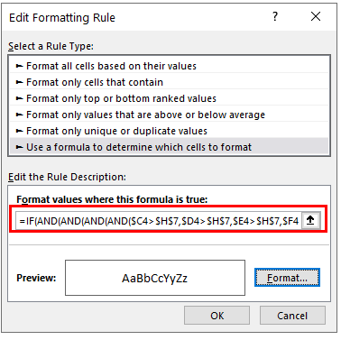
- You need to use a mixed reference in this formula ($C3, $D3, $E3, $F3) in order to lock the column but make the row relative – this will enable the formatting to format the entire row instead of just a single cell that meets the criteria.
- When the rule is evaluated, each column is evaluated by a nested IF statement – and if all the IF statements are true, then a TRUE is returned, and the entire row is highlighted. As you are applying the formula to a range of columns and rows, the row changes relatively, but the column will always remain the same.
- Click on the Format button and select your desired formatting.
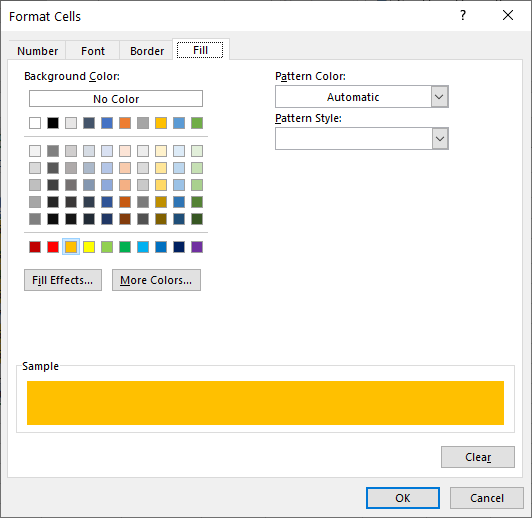
- Click OK, and then OK once again to return to the Conditional Formatting Rules Manager.
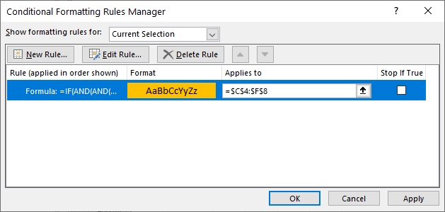
- Click Apply to apply the formatting to your selected range and then click Close.
Every row in the range selected that has a cell with a value greater than 5 will have its background color changed to yellow.
ISERROR Function
To highlight a row if there is a cell with an error in it in the row with conditional formatting, you can use the ISERROR Function within a Conditional Formatting rule.
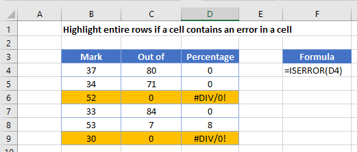
- Select the range you want to apply formatting to.
- In the Ribbon, select Home > Conditional Formatting > New Rule.
- Select Use a formula to determine which cells to format, and enter the following formula:
=ISERROR($D4)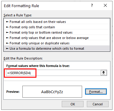
- You need to use a mixed reference to make sure that the column is locked and that the row is relative – this will enable the formatting to format the entire row instead of just a single cell that meets the criteria.
- When the rule is evaluated for all the cells in the range, the row will change but the column will remain the same. This causes the rule to ignore the values in any of the other columns and just concentrate on the values in Column D. As long as the rows match, and Column D of that row returns an error, then the formula result is TRUE and the formatting is applied for the whole row.
- Click on the Format button and select your desired formatting.
- Click OK, and then OK once again to return to the Conditional Formatting Rules Manager.
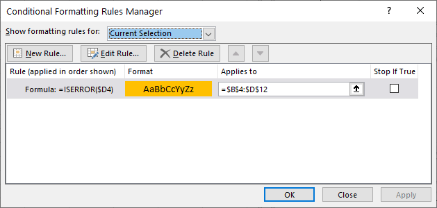
- Click Apply to apply the formatting to your selected range and then click Close.
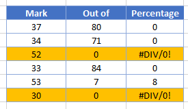
Every row in the range selected that has a cell with an error in it has its background color changed to yellow.
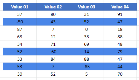
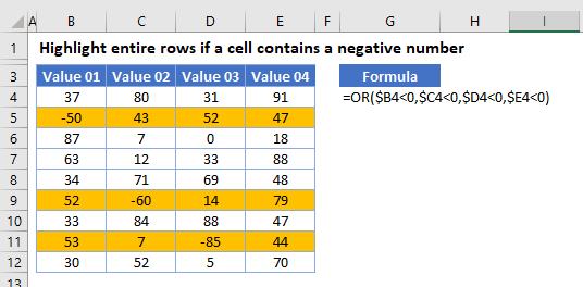
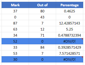
Evaluate for Negative Numbers
To highlight a row if there is a cell with a negative number in it in the row with conditional formatting, you can use the OR Function within a Conditional Formatting rule.
- Select the range you want to apply formatting to.
- In the Ribbon, select Home > Conditional Formatting > New Rule.
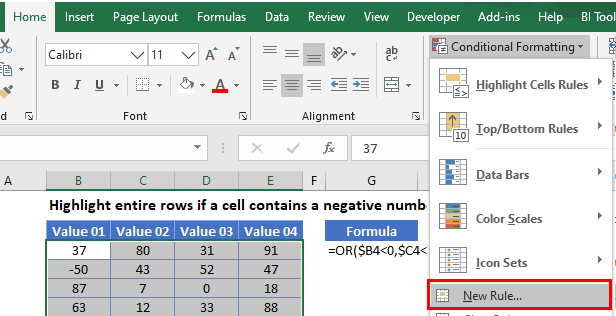
- Select Use a formula to determine which cells to format, and enter the formula:
=OR($B4<0,$C4<0,$D4<0,$E4<0)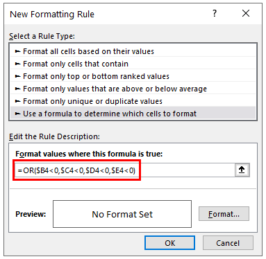
- You need to use a mixed reference to make sure that the column is locked and that the row is relative – this will enable the formatting to format the entire row instead of just a single cell that meets the criteria.
- When the rule is evaluated, each column is evaluated by the OR statement – and if all the OR statements are true, then a TRUE is returned. If a TRUE is returned, then the entire formula will return true and the entire row is highlighted. As you are applying the formula to a range of columns and rows, as the row changes, the row in the will change relatively, but the column will always remain the same.
- Click on the Format button and select your desired formatting.
- Click OK, and then OK once again to return to the Conditional Formatting Rules Manager.
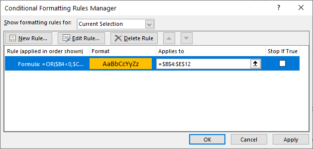
- Click Apply to apply the formatting to your selected range and then click Close.
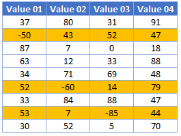
Every row in the range selected that has a cell with a negative number will have its background color changed to yellow.
Conditional Format If in Google Sheets
The process to highlight rows based on the value contained in that cell in Google Sheets is similar to the process in Excel.
- Highlight the cells you wish to format, and then click on Format > Conditional Formatting.
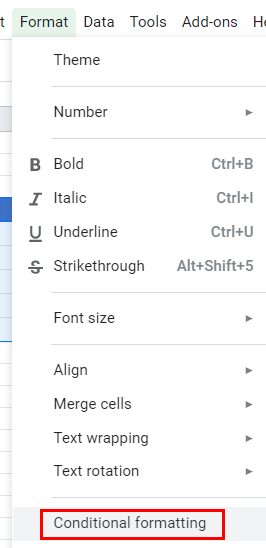
- The Apply to Range section will already be filled in.

- From the Format Rules section, select Custom Formula.
- Type in the following formula.
=IF(AND(AND(AND(AND($C3>$H$6,$D3>$H$6,$E3>$H$6, ,$F3>$H$6)))),TRUE,FALSE)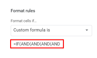
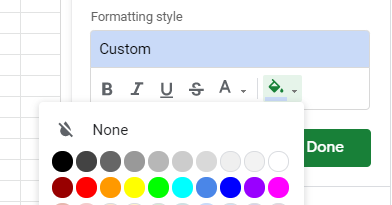
- Select the fill style for the cells that meet the criteria.
- Click Done to apply the rule.
See also: IF Formula – Set Cell Color w/ Conditional Formatting.
If There Is an Error
The process to highlight rows where an error is contained in a cell in the row in Google Sheets is similar to the process in Excel.
- Highlight the cells you wish to format, and then click on Format, Conditional Formatting.
- The Apply to Range section will already be filled in.
- From the Format Rules section, select Custom Formula.
- Type in the following formula:
=ISERROR(D4)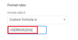
- Select the fill style for the cells that meet the criteria.
- Click Done to apply the rule.
Evaluate for Negative Numbers
The process to highlight rows if there is a cell with a negative number in it in the row with conditional formatting sheets is similar to the process in Excel.
- Highlight the cells you wish to format, and then click on Format > Conditional Formatting.
- The Apply to Range section will already be filled in.
- From the Format Rules section, select Custom Formula.
- Type the following formula.
=OR($B4<0,$C4<0,$D4<0,$E4<0)
- Select the fill style for the cells that meet the criteria.
- Click Done to apply the rule.