
Name a cell
-
Select a cell.
-
In the Name Box, type a name.

-
Press Enter.
To reference this value in another table, type th equal sign (=) and the Name, then select Enter.
Define names from a selected range
-
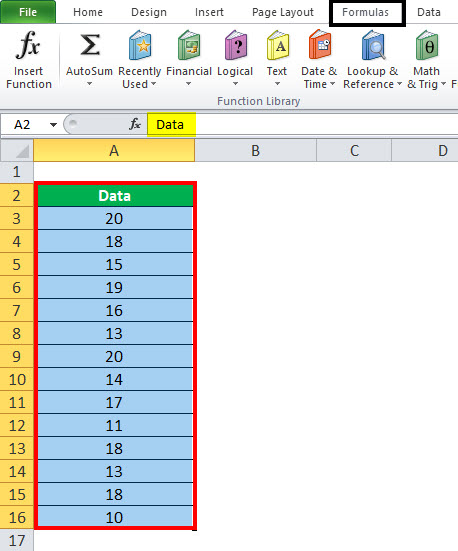
Select the range you want to name, including the row or column labels.
-
Select Formulas > Create from Selection.
-
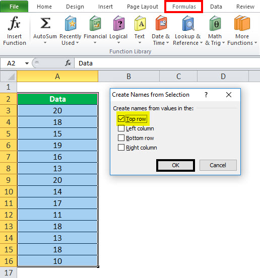
In the Create Names from Selection dialog box, designate the location that contains the labels by selecting the Top row, Left column, Bottom row, or Right column check box.
-
Select OK.
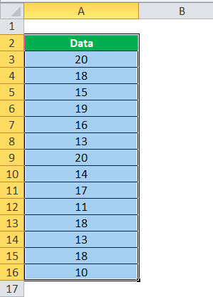
Excel names the cells based on the labels in the range you designated.
Use names in formulas
-
Select a cell and enter a formula.
-
Place the cursor where you want to use the name in that formula.
-
Type the first letter of the name, and select the name from the list that appears.
Or, select Formulas > Use in Formula and select the name you want to use.
-
Press Enter.
Manage names in your workbook with Name Manager
-
On the ribbon, go to Formulas > Name Manager. You can then create, edit, delete, and find all the names used in the workbook.
Name a cell
-
Select a cell.
-
In the Name Box, type a name.
-
Press Enter.
Define names from a selected range
-
Select the range you want to name, including the row or column labels.
-
Select Formulas > Create from Selection.
-
In the Create Names from Selection dialog box, designate the location that contains the labels by selecting the Top row,Left column, Bottom row, or Right column check box.
-
Select OK.
Excel names the cells based on the labels in the range you designated.
Use names in formulas
-
Select a cell and enter a formula.
-
Place the cursor where you want to use the name in that formula.
-
Type the first letter of the name, and select the name from the list that appears.
Or, select Formulas > Use in Formula and select the name you want to use.
-
Press Enter.
Manage names in your workbook with Name Manager
-
On the Ribbon, go to Formulas > Defined Names > Name Manager. You can then create, edit, delete, and find all the names used in the workbook.
In Excel for the web, you can use the named ranges you’ve defined in Excel for Windows or Mac. Select a name from the Name Box to go to the range’s location, or use the Named Range in a formula.
For now, creating a new Named Range in Excel for the web is not available.
Rows and Column in Excel (Table of Contents)
- Introduction to Rows and Column in Excel
- Rows and Column Navigation in excel
- How to Select Rows and Column in excel?
- Adjusting Column Width
Introduction to Rows and Column in Excel
In Microsoft excel, if we open a new workbook, we can see that sheet will contain tables with light grey color. Basically excel is a tabular format which contains n number of rows and columns, where rows in excel will be in a horizontal line, and column in excel will be in a vertical line.
- In excel, we can find each row by its row number, which is shown in the below screenshot, which shows vertical numbers on the left side of each sheet.
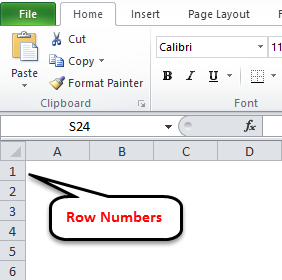
- As we can see in the above screenshot that each row can be identified by their row numbers like 1, 2, 3 etc.
- Whereas we can find the column in excel, which can be identified by the column header like A, B, C. which will be shown normally in all excel sheets, which are shown below.
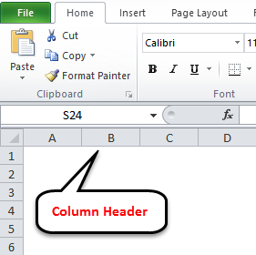
- In Excel, each column is named by its header, which shows the column header horizontally at the top of the excel sheet.
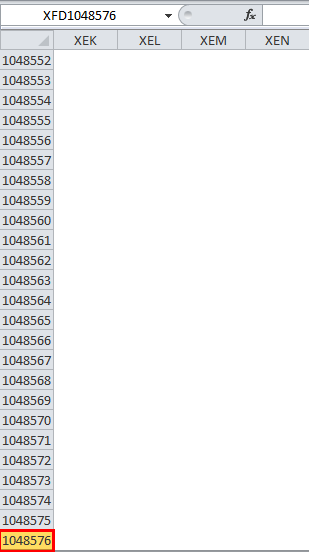
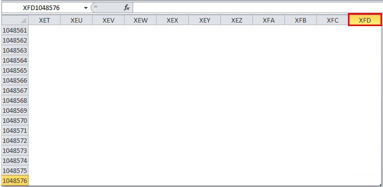
In Microsoft Excel 2010 and the latest version, we have row numbers ranging from 1 to 1048576 in 1048576, whereas the column ranges from A to XFD in a total of 16384 columns which is shown in the below screenshot.
Rows in excel range from 1 to 1048576, which is highlighted in red mark
The column in excel ranges from A to XFD, which is highlighted in red mark.
Rows and Column Navigation in excel
In this example, we will see how to navigate rows and columns with the below examples.
We can find the last row of excel by using the keyboard shortcut key CTRL+DOWN NAVIGATION ARROW KEY, or else we can use the vertical scrollbars to go to the end of the row.
We can find the last column of excel by using the CTRL+RIGHT NAVIGATION ARROW KEY, or else we can use the horizontal scrollbars to go to the end of the column.
How to Select Rows and Column in excel?
In this example, we will learn how to select the rows and columns in excel.
You can download this Rows and Column Excel Template here – Rows and Column Excel Template
Rows and Column in Excel – Example#1
Normally, when we open a workbook, we can see that sheet contains tabular rows and columns where each row is specified by their row number and column specified by their column header.
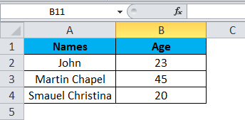
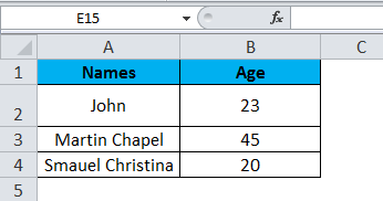
Consider the below example, which has some data in an excel sheet. Here we will see how to select the rows and columns.
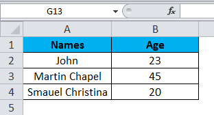
In the above screenshot, we can see that names and age column have their own header name A and B, and each row has its own row number.
In excel, each time when we select a row or column, “Name Box” will display the specific row number and column name, which is shown in the below screenshot.
In this example, we will select the Names and Age, and let’s see how the rows and column header is getting displayed.
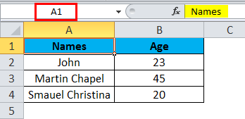
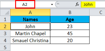
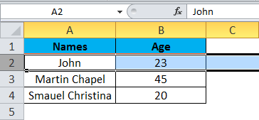
Step 1 – First, select the cell Name John.
Step 2 – Once you select the cell name, John, we will get the row number and column name as A2 in the name box, which means that we have selected A column second row as A2, shown below screenshot with yellow highlighted.
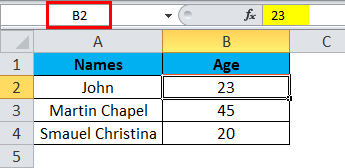
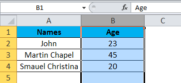
Step 3 – Now select cell 23, where it will show the selected cell is B2 which is shown in the below screenshot with yellow highlighted.
Step 4 – Now select all the names and columns to show that we have 4 rows and 2 columns shown in the below screenshot.
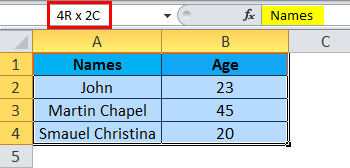
In this way, we can identify the row number and column name by selecting each cell in excel.
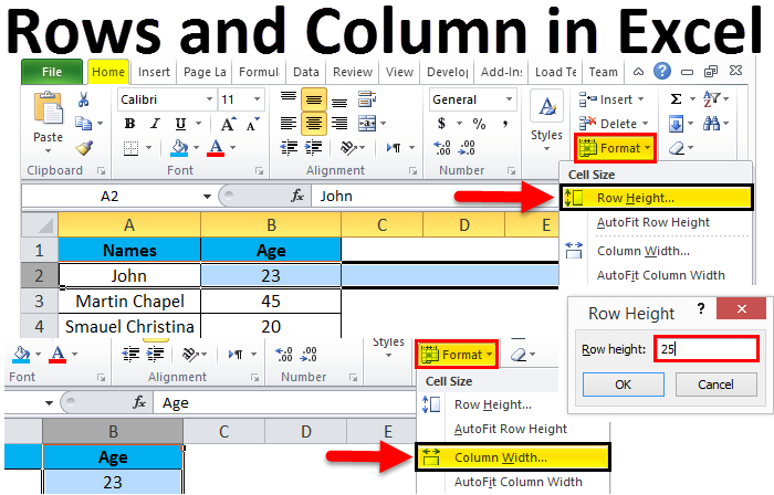
Example#2 – Changing Row and Column Size
This example shows how to change the row and column size by using the following examples.
Excel row and column width size can be modified by using the format option in the HOME menu, which is shown below.
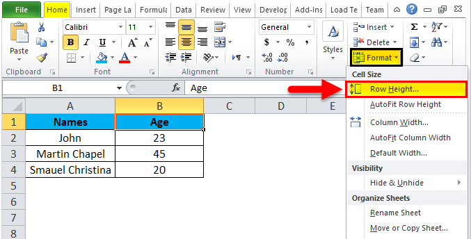
Using the format menu, we can change the row and column width where we have the list option, which are as follows:
- ROW HEIGHT– This is used to adjust the row height.
- AUTOFIT ROW HEIGHT– This will automatically adjust the row height.
- COLUMN WIDTH – This is used to adjust column width.
- AUTOFIT COLUMN WIDTH– This will automatically adjust the column width.
Let’s consider the below example to change the row and column width. Follow the below steps.
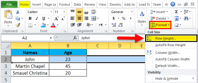
Step 1 – First, select the second row as shown in the below screenshot.
Step 2 – Go to the Format menu and click on ROW HEIGHT, as shown below.
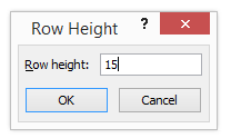
Step 3 – Once we select the ROW HEIGHT, we will get the below dialog box to change the height of the row.
Step 4 – Now increase the row height to 25 so that the selected row height will get increased, as shown in the below screenshot.

We can see that row height has been increased when compared to the previous one; alternatively, we can change the row height by using the mouse.
Step 5 – Now go to the second option in the format list called AUTOFIT ROW HEIGHT, which will automatically reset the row to its original height.
Step 6 – Select the same row and go to the Format menu.
Step 7 – Now select the “AutoFit Row Height” as shown below.
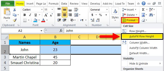
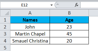
Once we click on the “AutoFit Row Height” option, the row height will reset to the original position, shown below.
Adjusting Column Width
We can adjust the column width in the same way by using the format option.
Step 1 – First, click on the cell B cell as shown below.
Step 2 – Now go to the Format menu and click on column width as shown in the below screenshot.
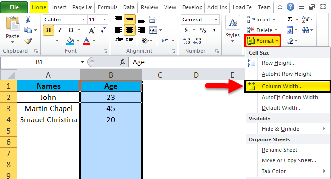
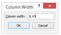
Once we click on the Column width, we will get the below dialog box to increase the column width, as shown below.
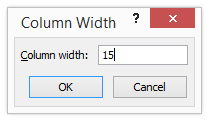
Step 3 – Now increase the column width by 15 to increase the selected column width.
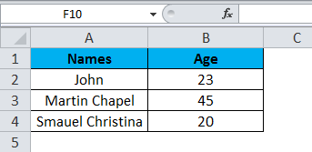
In the above screenshot, we can see that column width has been increased; alternatively, we can adjust the column width by using the mouse where if we place the mouse cursor, we will get the + plus mark sign near to the column.
Step 4 – Now click on the next option called “AutoFit Column width”. So that the selected column will get reset to its original size, which is shown below.
Things to Remember
- In excel, we can delete and insert multiple rows and columns.
- We can hide the specific row and columns using the hide option.
- Row and column cells can be protected by locking the specific cells.
Recommended Articles
This has been a guide to Rows and Columns in Excel. Here we also discuss Rows and Columns in Excel along with practical examples and downloadable excel template. You can also go through our other suggested articles –
- Excel Compare Two Columns
- Unhide Columns in Excel
- Sort Columns in Excel
- Excel Columns to Rows
MS-Excel / Excel 2003
Instead of taking the time to use individual descriptive names to assign names to ranges in a standard data table, it’s almost always more efficient to have
Excel do all the naming for you by using a table’s existing row and column headings.
To do this, select the table (including the cells with the row and column heading you want assigned) and then choose Insert → Name → Create to open the
Create Names dialog box.
When you first open the Create Names dialog box, Excel automatically selects both the Top Row and Left Column check boxes:
- When the Top Row check box is selected, Excel assigns the column headings in the first row of your cell selection to the columns of data in the table.
- When the Left Column check box is selected, the program assigns the row headings in the first column of the cell selection to the rows of the table.
(It also assigns the row heading in the top row of the leftmost column to all the rows of data in the entire table.)
If the top row of your table doesn’t contain column headings, clear the Top Row check box. Likewise, if its first column doesn’t contain row headings, clear
the Left Column check box. Also, if your table uses an unusual layout in which the bottom row contains the column headings, clear the Top Row check box
and select the Bottom Row one instead. Finally, if the rightmost column of your table contains the row headings, clear the Left Column check box and
select the Right Column one in its place.
The range names you assign with the Create Names feature refer only to cells that contain data of the table and do not include the row
and column headings at the top and left or bottom and right of the cell selection.
All the range names you assign with Create Names are added to the Name Box dropdown list (on the Formula bar), meaning that
you can select their ranges in the worksheet simply by clicking their names on this dropdown list.
When assigning descriptive names to cell ranges in the Define Name dialog box, you never have to include the sheet name; just
make sure that the descriptive names are unique. Likewise, when referring to range names in formulas, don’t take time to add the
sheet reference because Excel keeps track of this automatically.

What is Name Range in Excel?
The name range in Excel is the range that has been given a name for future reference. To make a range as a named range, select the range of data and then insert a table. Then, we put a name to the range from the Name Box on the left-hand side of the window. After this, we can refer to the range by its name in any formula.
The name range in Excel makes it much cooler to keep track of things, especially when using formulas. You can assign a name to a range. No problem with any change in that range; you need to update the range from the Name Manager in ExcelThe name manager in Excel is used to create, edit, and delete named ranges. For example, we sometimes use names instead of giving cell references. By using the name manager, we can create a new reference, edit it, or delete it.read more. You do not need to update every formula manually. Similarly, you can create a name for a formula. Then, if you want to use that formula in another formula or another location, refer to it by name.
- The name ranges are significant because you can put any names in your formulas without considering cell references/addresses. Furthermore, you can assign the range with any name.
- Create a named range for any data or a named constant and use these names in your formulas in place of data references. In this way, you can make your formulas easier to comprehend better. A named range is just a human-understandable name for a range of cells in Excel.
- Using the name range in Excel, you can simplify and comprehend your formulas better. For example, you can assign a name for a range in an excel sheet for a function, a constant, or table data. Once you start using the names in your Excel sheet, you can easily understand these names.
Table of contents
- What is Name Range in Excel?
- Define Names For a Selected Range
- Excel names the cells based on the labels in the range you designated.
- Update named ranges in the Name Manager (Control + F3)
- How to Use Name Range in Excel?
- Example #1 Create a name by using the Define Name option
- Example #2 Make a named range by using Excel Name Manager
- Name Range using VBA.
- Things to Remember
- Recommended Articles
- Define Names For a Selected Range
Define Names For a Selected Range
- Select the data range you want to assign a name, then select formulas and create from the selection.
- Click on the “Create Names from Selection,” then select the “Top row,” “Left column,” “Bottom row,” or “Right column” checkbox and select “OK.”
Excel names the cells based on the labels in the range you designated.
- Use names in formulas, then select a cell and enter a formula.
- Place the cursor where you want to use the name range formula.
- Type the first letter of the name, and select the name from the list that appears.
- Or, select “Formulas,” then use in formula and select the name you want to use.
- Press the “Enter” key.
Update named ranges in the Name Manager (Control + F3)
You can update the name from the Name Manager. Press “Ctrl” and “F3” to update the name. Select the name you want to change, then change the reference range directly.
How to Use Name Range in Excel?
Let us understand the working of conditional formatting by simple Excel examples.
You can download this Using Names in Excel Template here – Using Names in Excel Template
Example #1 Create a name by using the Define Name option
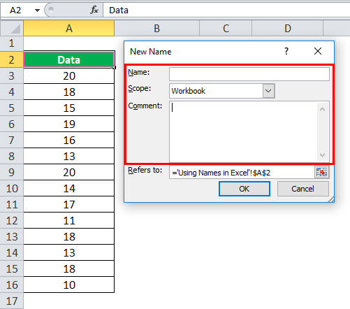
Below are the steps to create a name by using the “Define Name” option:
- First, select the cell(s).

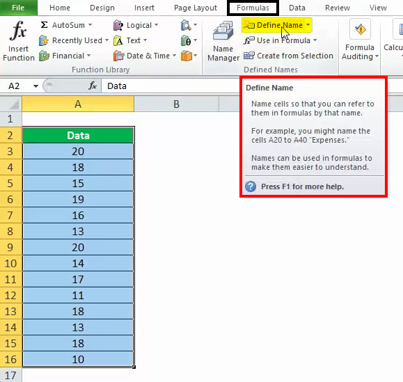
- On the “Formulas” tab, click the “Define Name” in the “Defined Names” group.

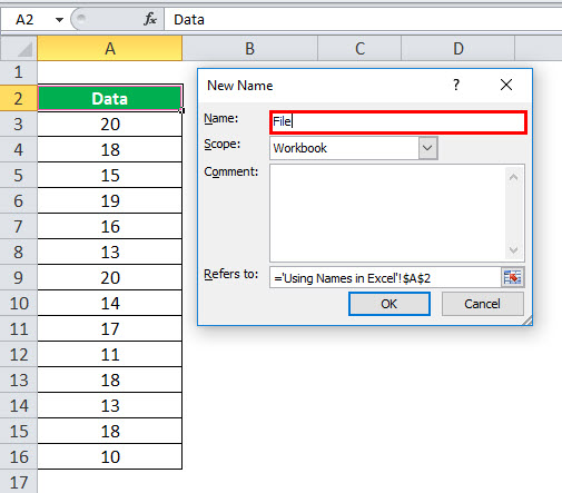
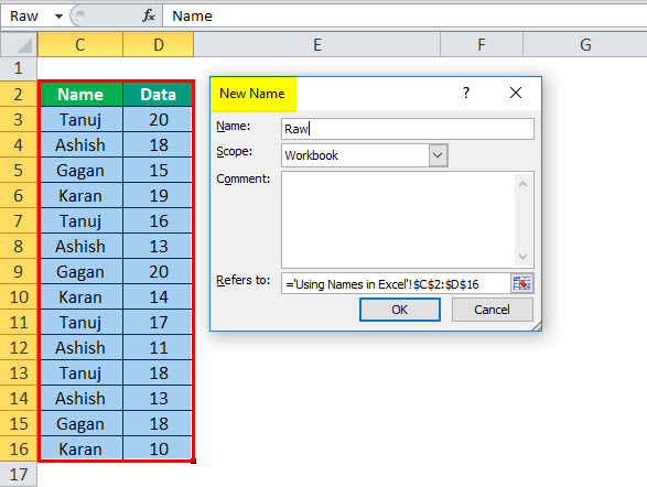
- In the “New Name” dialog box, specify three things:

- First, in the “Name” box, type the range name.

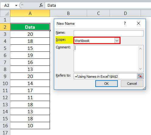
- In the “Scope” drop-down, set the name scope (Workbook by default).

- In the “Refers to” box, check the reference and correct it if needed. Finally, click “OK” to save the changes and close the dialog box.


Example #2 Make a named range by using Excel Name Manager
- Go to the “Formulas” tab, then the “Defined Names” group, and click the “Name Manager” or press “Ctrl + F3” (the preferred way).
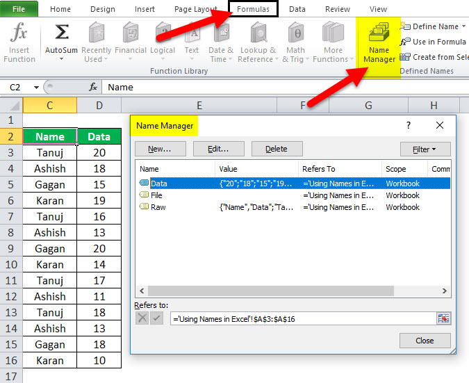
- In the top left-hand corner of the “Name Manager” dialog window, click the “New… button:”
Name Range using VBA.
We can apply the naming in VBA; here is the example as follows:
Sub sbNameRange()
‘Adding a Name
Names.Add Name:=”myData”, RefersTo:=”=Sheet1!$A$1:$A$10″
‘OR
‘You can use Name property of a Range.
Sheet1.Range(“$A$1:$A$10”).Name = “myData”
End Sub
Things to Remember
We must follow the below instruction while using the name range.
- The names can start with a letter, backslash (), or an underscore (_).
- The name should be under 255 characters long.
- The names must be continuous and cannot contain spaces and most punctuation characters.
- There must be no conflict with cell references in names using in excelCell reference in excel is referring the other cells to a cell to use its values or properties. For instance, if we have data in cell A2 and want to use that in cell A1, use =A2 in cell A1, and this will copy the A2 value in A1.read more.
- We can use single letters as names, but the letters “r” and “c” are reserved in Excel.
- The names are not case-sensitive – “Tanuj”, “TANUJ”, and “TaNuJ” are all the same in Excel.
Recommended Articles
This article is a guide to the Name Range in Excel. We discuss using names in Excel, practical examples, and downloadable Excel templates here. You also may look at these useful functions in Excel: –
- VBA RangeRange is a property in VBA that helps specify a particular cell, a range of cells, a row, a column, or a three-dimensional range. In the context of the Excel worksheet, the VBA range object includes a single cell or multiple cells spread across various rows and columns.read more
- Data Tables ExcelA data table in excel is a type of what-if analysis tool that allows you to compare variables and see how they impact the result and overall data. It can be found under the data tab in the what-if analysis section.read more
- Data Validation using ExcelThe data validation in excel helps control the kind of input entered by a user in the worksheet.read more
- Paste SpecialPaste special in Excel allows you to paste partial aspects of the data copied. There are several ways to paste special in Excel, including right-clicking on the target cell and selecting paste special, or using a shortcut such as CTRL+ALT+V or ALT+E+S.read more
XlsxWriter supports two forms of notation to designate the position of cells:
Row-column notation and A1 notation.
Row-column notation uses a zero based index for both row and column while A1
notation uses the standard Excel alphanumeric sequence of column letter and
1-based row. For example:
(0, 0)      # Row-column notation.
('A1')      # The same cell in A1 notation.

(6, 2)      # Row-column notation.
('C7')      # The same cell in A1 notation.
Row-column notation is useful if you are referring to cells programmatically:
for row in range(0, 5):
    worksheet.write(row, 0, 'Hello')
A1 notation is useful for setting up a worksheet manually and for working with
formulas:
worksheet.write('H1', 200)
worksheet.write('H2', '=H1+1')
In general when using the XlsxWriter module you can use A1 notation anywhere
you can use row-column notation. This also applies to methods that take a
range of cells:
worksheet.merge_range(2, 1, 3, 3, 'Merged Cells', merge_format)
worksheet.merge_range('B3:D4',    'Merged Cells', merge_format)
XlsxWriter supports Excel’s worksheet limits of 1,048,576 rows by 16,384
columns.
Note
- Ranges in A1 notation must be in uppercase, like in Excel.
- In Excel it is also possible to use R1C1 notation. This is not
supported by XlsxWriter.
Row and Column Ranges
In Excel you can specify row or column ranges such as 1:1 for all of the
first row or A:A for all of the first column. In XlsxWriter these can be
set by specifying the full cell range for the row or column:
worksheet.print_area('A1:XFD1')      # Same as 1:1
worksheet.print_area('A1:A1048576')  # Same as A:A
This is actually how Excel stores ranges such as 1:1 and A:A
internally.
These ranges can also be specified using row-column notation, as explained
above:
worksheet.print_area(0, 0,       0, 16383)  # Same as 1:1
worksheet.print_area(0, 0, 1048575,     0)  # Same as A:A
To select the entire worksheet range you can specify
A1:XFD1048576.
Relative and Absolute cell references
When dealing with Excel cell references it is important to distinguish between
relative and absolute cell references in Excel.
Relative cell references change when they are copied while Absolute
references maintain fixed row and/or column references. In Excel absolute
references are prefixed by the dollar symbol as shown below:
'A1'    # Column and row are relative.
'$A1'   # Column is absolute and row is relative.
'A$1'   # Column is relative and row is absolute.
'$A$1'  # Column and row are absolute.
See the Microsoft Office documentation for
more information on relative and absolute references.
Some functions such as conditional_format() may require absolute
references, depending on the range being specified.
Defined Names and Named Ranges
It is also possible to define and use “Defined names/Named ranges” in
workbooks and worksheets, see define_name():
workbook.define_name('Exchange_rate', '=0.96')
worksheet.write('B3', '=B2*Exchange_rate')
See also Example: Defined names/Named ranges.
Cell Utility Functions
The XlsxWriter utility module contains several helper functions for
dealing with A1 notation as shown below. These functions can be imported as
follows:
from xlsxwriter.utility import xl_rowcol_to_cell

cell = xl_rowcol_to_cell(1, 2)  # C2
xl_rowcol_to_cell()
-
xl_rowcol_to_cell(row, col[, row_abs, col_abs]) -
Convert a zero indexed row and column cell reference to a A1 style string.
Parameters: - row (int) – The cell row.
- col (int) – The cell column.
- row_abs (bool) – Optional flag to make the row absolute.
- col_abs (bool) – Optional flag to make the column absolute.
Return type: A1 style string.
The xl_rowcol_to_cell() function converts a zero indexed row and column
cell values to an A1 style string:
cell = xl_rowcol_to_cell(0, 0)   # A1
cell = xl_rowcol_to_cell(0, 1)   # B1
cell = xl_rowcol_to_cell(1, 0)   # A2
The optional parameters row_abs and col_abs can be used to indicate
that the row or column is absolute:
str = xl_rowcol_to_cell(0, 0, col_abs=True)                # $A1
str = xl_rowcol_to_cell(0, 0, row_abs=True)                # A$1
str = xl_rowcol_to_cell(0, 0, row_abs=True, col_abs=True)  # $A$1
xl_cell_to_rowcol()
-
xl_cell_to_rowcol(cell_str) -
Convert a cell reference in A1 notation to a zero indexed row and column.
Parameters: cell_str (string) – A1 style string, absolute or relative. Return type: Tuple of ints for (row, col)
The xl_cell_to_rowcol() function converts an Excel cell reference in A1
notation to a zero based row and column. The function will also handle Excel’s
absolute, $, cell notation:
(row, col) = xl_cell_to_rowcol('A1')    # (0, 0)
(row, col) = xl_cell_to_rowcol('B1')    # (0, 1)
(row, col) = xl_cell_to_rowcol('C2')    # (1, 2)
(row, col) = xl_cell_to_rowcol('$C2')   # (1, 2)
(row, col) = xl_cell_to_rowcol('C$2')   # (1, 2)
(row, col) = xl_cell_to_rowcol('$C$2')  # (1, 2)
xl_col_to_name()
-
xl_col_to_name(col[, col_abs]) -
Convert a zero indexed column cell reference to a string.
Parameters: - col (int) – The cell column.
- col_abs (bool) – Optional flag to make the column absolute.
Return type: Column style string.
The xl_col_to_name() converts a zero based column reference to a string:
column = xl_col_to_name(0)    # A
column = xl_col_to_name(1)    # B
column = xl_col_to_name(702)  # AAA
The optional parameter col_abs can be used to indicate if the column is
absolute:
column = xl_col_to_name(0, False)  # A
column = xl_col_to_name(0, True)   # $A
column = xl_col_to_name(1, True)   # $B
xl_range()
-
xl_range(first_row, first_col, last_row, last_col) -
Converts zero indexed row and column cell references to a A1:B1 range
string.Parameters: - first_row (int) – The first cell row.
- first_col (int) – The first cell column.
- last_row (int) – The last cell row.
- last_col (int) – The last cell column.
Return type: A1:B1 style range string.
The xl_range() function converts zero based row and column cell references
to an A1:B1 style range string:
cell_range = xl_range(0, 0, 9, 0)  # A1:A10
cell_range = xl_range(1, 2, 8, 2)  # C2:C9
cell_range = xl_range(0, 0, 3, 4)  # A1:E4
cell_range = xl_range(0, 0, 0, 0)  # A1
xl_range_abs()
-
xl_range_abs(first_row, first_col, last_row, last_col) -
Converts zero indexed row and column cell references to a $A$1:$B$1
absolute range string.Parameters: - first_row (int) – The first cell row.
- first_col (int) – The first cell column.
- last_row (int) – The last cell row.
- last_col (int) – The last cell column.
Return type: $A$1:$B$1 style range string.
The xl_range_abs() function converts zero based row and column cell
references to an absolute $A$1:$B$1 style range string:
cell_range = xl_range_abs(0, 0, 9, 0)  # $A$1:$A$10
cell_range = xl_range_abs(1, 2, 8, 2)  # $C$2:$C$9
cell_range = xl_range_abs(0, 0, 3, 4)  # $A$1:$E$4
cell_range = xl_range_abs(0, 0, 0, 0)  # $A$1