Row count for excel - Word и Excel - помощь в работе с программами

Excel for Microsoft 365 Excel for Microsoft 365 for Mac Excel for the web Excel 2021 Excel 2021 for Mac Excel 2019 Excel 2019 for Mac Excel 2016 Excel 2016 for Mac Excel 2013 More…Less

If you need a quick way to count rows that contain data, select all the cells in the first column of that data (it may not be column A). Just click the column header. The status bar, in the lower-right corner of your Excel window, will tell you the row count.

Do the same thing to count columns, but this time click the row selector at the left end of the row.

The status bar then displays a count, something like this:

If you select an entire row or column, Excel counts just the cells that contain data. If you select a block of cells, it counts the number of cells you selected. If the row or column you select contains only one cell with data, the status bar stays blank.

Notes:

If you need to count the characters in cells, see Count characters in cells.
If you want to know how many cells have data, see Use COUNTA to count cells that aren’t blank.
You can control the messages that appear in the status bar by right-clicking the status bar and clicking the item you want to see or remove. For more information, see Excel status bar options.

Need more help?

You can always ask an expert in the Excel Tech Community or get support in the Answers community.

Need more help?

Источник

How to Count the Number of Rows in Excel?

Here are the different ways of counting rows in Excel using the formula, rows with data, empty rows, rows with numerical values, rows with text values, and many other things related to counting the number of rows in Excel.

You can download this Count Rows Excel Template here – Count Rows Excel Template

How to Count the Number of Rows in Excel?
- #1 – Excel Count Rows which has only the Data
- #2 – Count all the rows that have the data
- #3 – Count the rows that only have the numbers
- #4 – Count Rows, which only has the Blanks
- #5 – Count rows that only have text values
- #6 – Count all of the rows in the range
- Things to Remember
- Recommended Articles

#1 – Excel Count Rows which has only the Data

Firstly, we will see how to count the number of rows in Excel with the data. There could be empty rows between the data, but we often need to ignore them and find exactly how many rows contain the data in it.

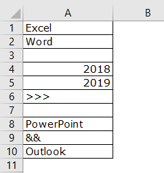
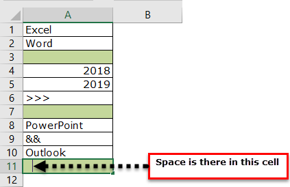
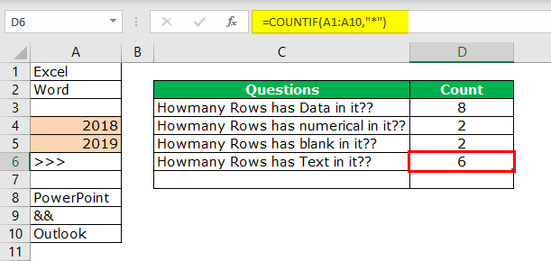
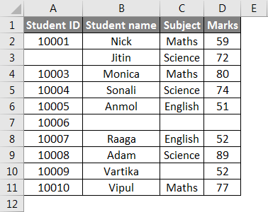
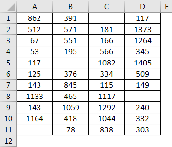
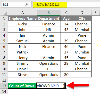
We can count the number of rows with data by selecting the range of cells in Excel. For example, take a look at the below data.

We have a total of 10 rows (border inserted area). In this 10 row, we want to count exactly how many cells have data. Since this is a small list of rows, we can easily calculate the number of rows. But when it comes to the huge database, it is impossible to count manually. So, this article will help you with this.
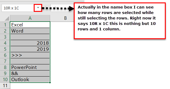
Firstly, we must select all the rows in Excel.
It is not telling us how many rows contain the data here. Instead, look at the Excel screen’s right-hand side bottom, i.e., a status bar.

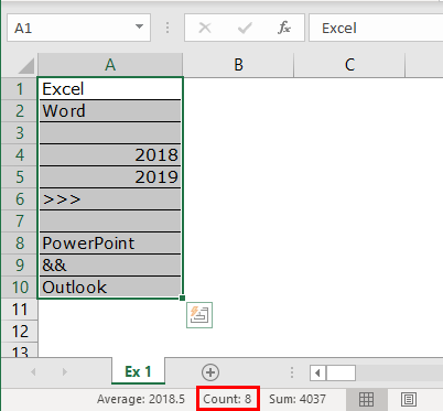
Take a look at the red circled area. It says COUNT as 8, which means that out of 10 selected rows, 8 have data.
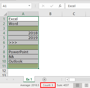
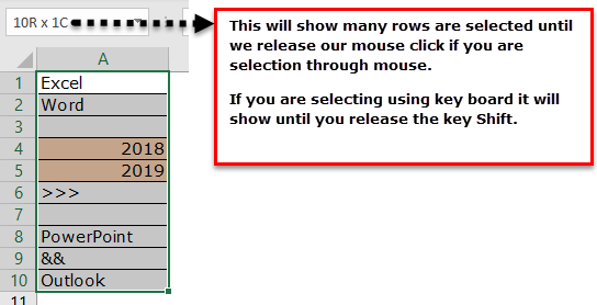
Now, we will select one more row in the range and see what the count will be.
We have selected 11 rows, but the count says 9, whereas we have data only in 8 rows. When we closely examine the cells, the 11th row contains a space.

Even though there is no value in the cell and it has only space Excel will be treated as the cell which contains the data.

#2 – Count all the rows that have the data

We know how to check how many rows contain the data quickly. But that is not the dynamic way of counting rows that have data. Instead, we need to apply the COUNTA function to count how many rows contain the data.

We will apply the COUNTA function in the D3 cell.

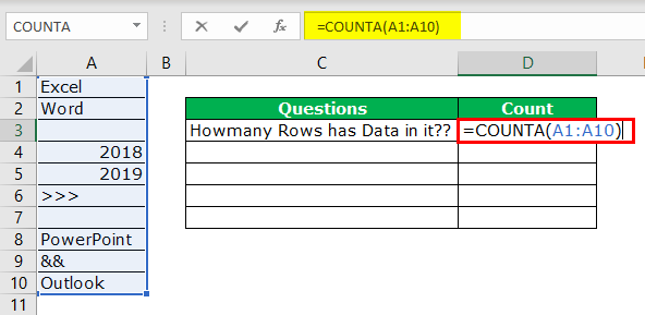
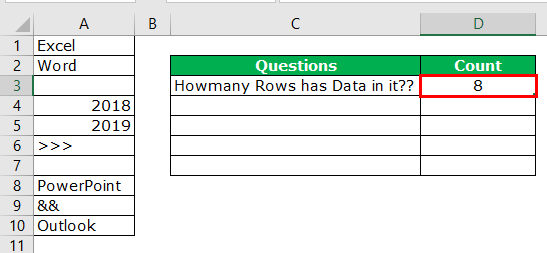
So, the total number of rows containing the data is 8 rows. Even this formula treats space as data.

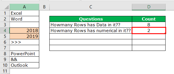
#3 – Count the rows that only have the numbers

Here we want to count how many rows contain only numerical values.

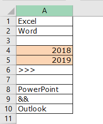
We can easily say 2 rows contain numerical values. Let us examine this by using a formula. We have a built-in formula called COUNT which counts only numerical values in the supplied range.

We will apply the COUNT function in cell B1 and select the range as A1 to A10.

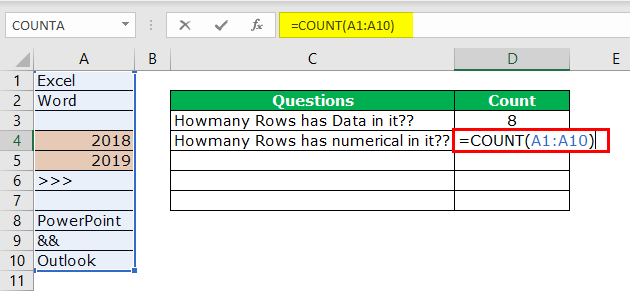
The COUNT function also says 2 as a result. So, out of 10 rows, only rows contain numerical values.

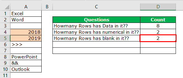
#4 – Count Rows, which only has the Blanks

We can find only blank rows by using the COUNTBLANK function in Excel.

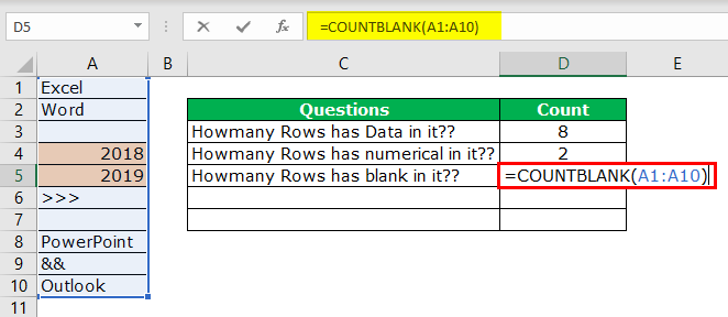
We have 2 blank rows in the selected range, which are revealed by the count blank function.

#5 – Count rows that only have text values

Remember, we do not have any straight in the COUNTTEXT function. Unlike in previous cases, we need to think differently here. We can use the COUNTIF functionThe COUNTIF function in Excel counts the number of cells within a range based on pre-defined criteria. It is used to count cells that include dates, numbers, or text. For example, COUNTIF(A1:A10,”Trump”) will count the number of cells within the range A1:A10 that contain the text “Trump”
read more with a wildcard character asterisk (*).

Here all the magic is done by the wildcard character asterisk (*). It matches any of the alphabets in the row and returns the result as a text value row. Even if the row contains numerical and text values, it will be treated as text value only.

#6 – Count all of the rows in the range

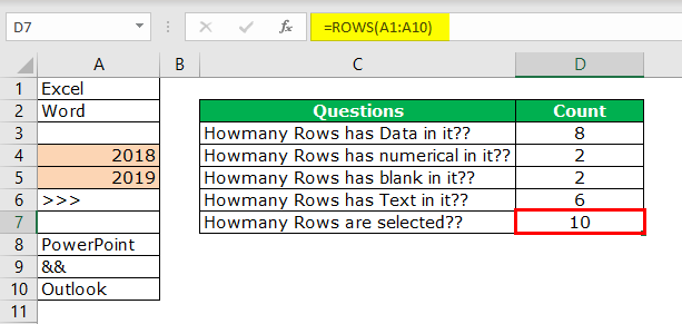
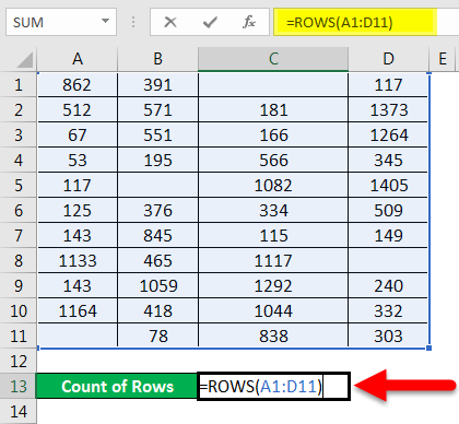
Now comes the important part. How do we count how many rows we have selected? One uses the Name Box in excel, which is limited while still choosing the rows. But how do we measure then?

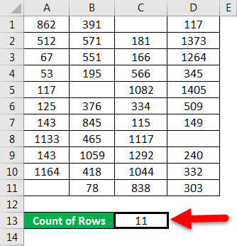
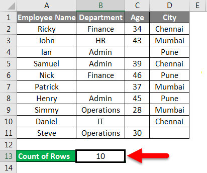
We have a built-in ROWS formula, which returns how many rows are selected.

Things to Remember

Even space is treated as a value in the cell.
If the cell contains numerical and text values, it will be treated as a text value.
ROW may return the current row we are in, but ROWS will return how many are in the supplied range even though there is no data in the rows.

Introduction to Row Count in Excel

Excel provides many built-in functions through which we can do multiple calculations. We can also count the rows and columns in Excel. Here in this article, we will discuss the Row Count in Excel. If we want to measure the rows which contain data, select all the cells of the first column by clicking on the column header. It will display the row count on the status bar in the lower right corner.

Let’s take some values in the Excel sheet.

Select the entire column which contains data. Now click on the column label for counting the rows; it will show you the row count. Refer to the below screenshot:

There are two types of functions for counting the rows.

ROW()
ROWS()

The ROW() function gives you the row number of a particular cell.

The ROWS() function gives you the count of rows in a range.

How to Count the Rows in Excel?

Let’s take some examples to understand the usage of ROWS functions.

You can download this Row Count Excel Template here – Row Count Excel Template

Example #1

We have given the below employee data.

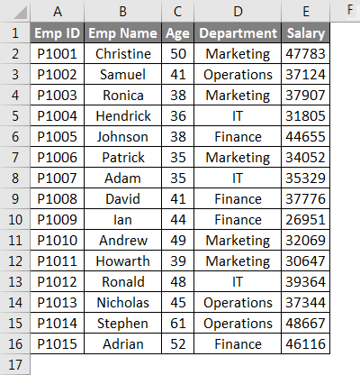
For counting the rows here, we will use the below function here:

=ROWS(range)

Where range = a range of cells containing data.

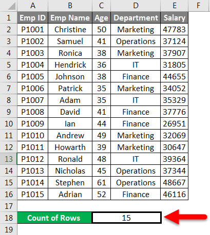
Now we will apply the above function like the below screenshot:

Which returns the number of rows containing the data in the supplied range.

The final result is given below:

Example #2

We have given below some student marks subject-wise.

As we can see in the above dataset, certain information is absent.

As per the screenshot below, we will apply the ROWS function for counting the rows containing data.

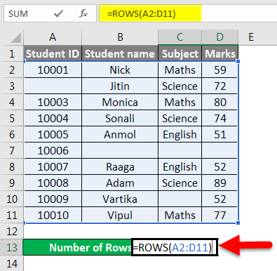
The final result is given below:

Example #3

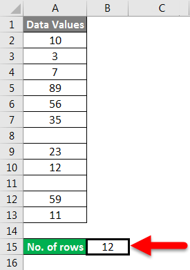
We have given the below data values.

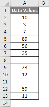
We will pass the range of data values within the function for counting the number of rows.

Apply the function like the below screenshot:

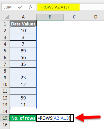
Press ENTER key here, and it will return the count of rows.

The final result is shown below:

Explanation:

When we pass the range of cells, it gives you the count of cells you selected.

Example #4

We have given below product details:

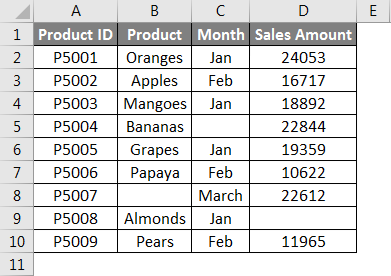
Now we will pass the range of the given dataset within the function like the below screenshot:

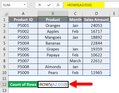
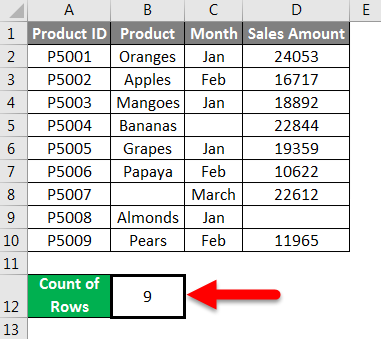
Press ENTER key, which will give you the count of rows containing data in the passing range.

The final result is given below:

Example #5

We have given some raw data.

Some cell values are missing here, so now, for counting the rows, we will apply the function shown in the below screenshot:

Hit the Enter key, and it will return the count of rows having data.

The final result is given below:

Example #6

We have given a company employee data where some details are missing:

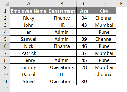
Now apply the ROWS function to count the row containing data of employees:

Hit the Enter key to get the final rows

Things to Remember About Row Count in Excel

When you click on the column heading for counting the rows, it will give you the count which contains data.
If you pass a range of cells, it will return the number of cells that you have selected.
The status bar won’t show you anything if the column contains the data only in one cell. That is, the status bar stays blank.
If the data are given in the table form, then for counting the rows, you can pass the table range within the ROWS function.
You can also do the setting of the message in the status bar. Do right-click on the status bar and click the item you want to see or remove.

Определение количества строк

Существует довольно большое количество способов определения количества строк. При их использовании применяются различные инструменты. Поэтому нужно смотреть конкретный случай, чтобы выбрать более подходящий вариант.

Способ 1: указатель в строке состояния

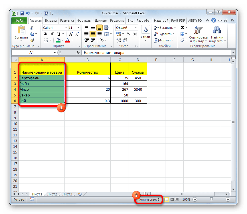
Самый простой способ решить поставленную задачу в выделенном диапазоне – это посмотреть количество в строке состояния. Для этого просто выделяем нужный диапазон. При этом важно учесть, что система считает каждую ячейку с данными за отдельную единицу. Поэтому, чтобы не произошло двойного подсчета, так как нам нужно узнать количество именно строк, выделяем только один столбец в исследуемой области. В строке состояния после слова «Количество» слева от кнопок переключения режимов отображения появится указание фактического количества заполненных элементов в выделенном диапазоне.

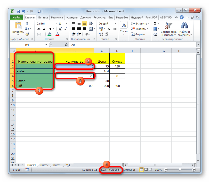
Правда, случается и такое, когда в таблице нет полностью заполненных столбцов, при этом в каждой строке имеются значения. В этом случае, если мы выделим только один столбец, то те элементы, у которых именно в той колонке нет значений, не попадут в расчет. Поэтому сразу выделяем полностью конкретный столбец, а затем, зажав кнопку Ctrl кликаем по заполненным ячейкам, в тех строчках, которые оказались пустыми в выделенной колонке. При этом выделяем не более одной ячейки на строку. Таким образом, в строке состояния будет отображено количество всех строчек в выделенном диапазоне, в которых хотя бы одна ячейка заполнена.

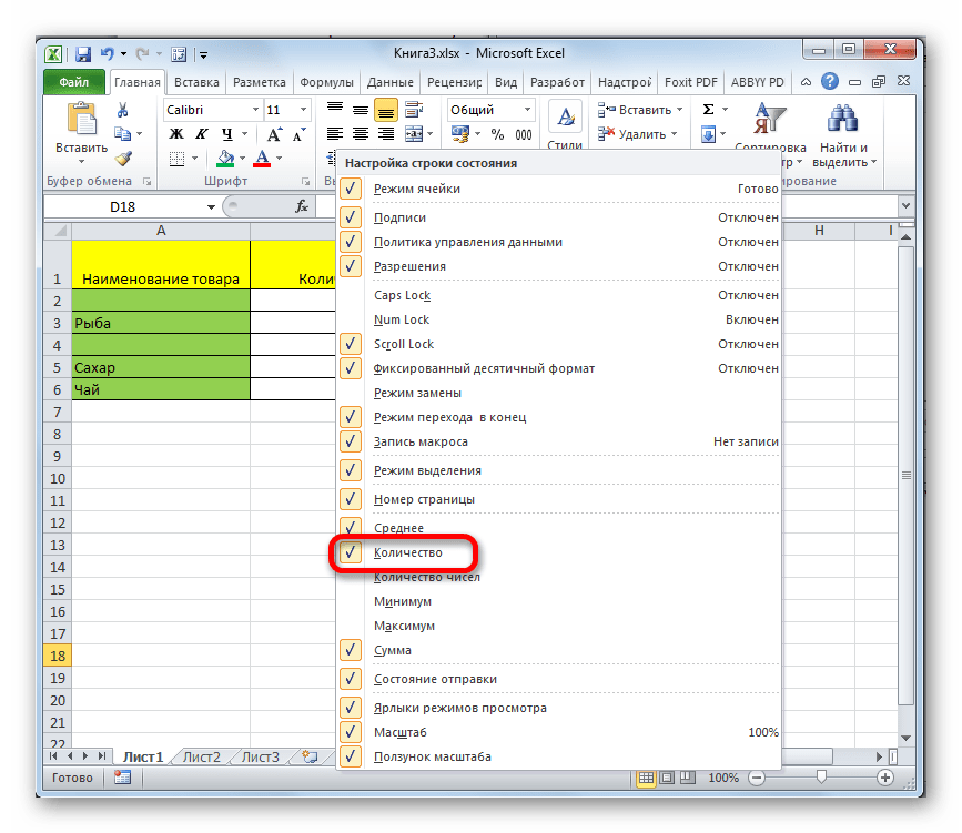
Но бывают и ситуации, когда вы выделяете заполненные ячейки в строках, а отображение количества на панели состояния так и не появляется. Это означает, что данная функция просто отключена. Для её включения кликаем правой кнопкой мыши по панели состояния и в появившемся меню устанавливаем галочку напротив значения «Количество». Теперь численность выделенных строк будет отображаться.

Способ 2: использование функции

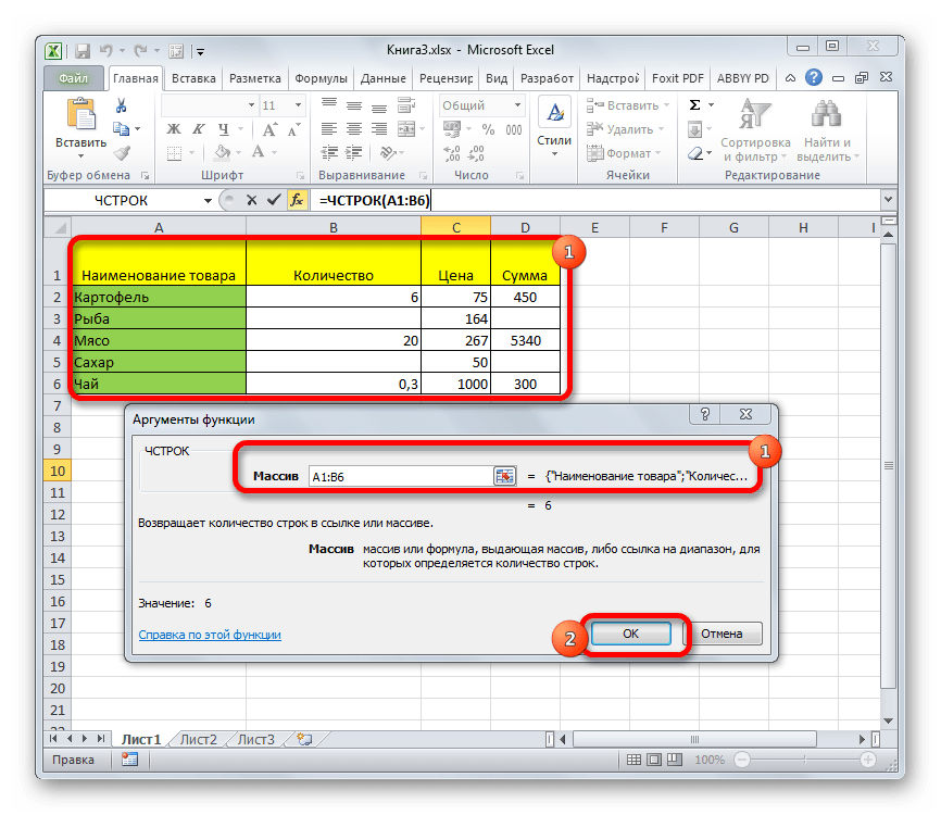
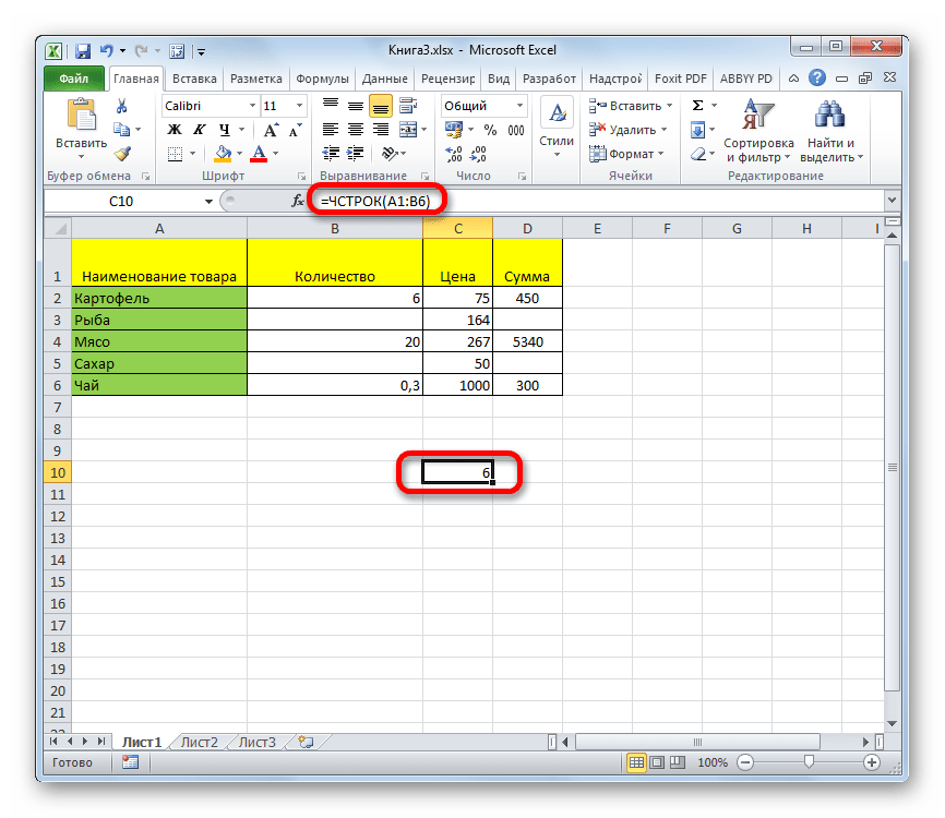
Но, вышеуказанный способ не позволяет зафиксировать результаты подсчета в конкретной области на листе. К тому же, он предоставляет возможность посчитать только те строки, в которых присутствуют значения, а в некоторых случаях нужно произвести подсчет всех элементов в совокупности, включая и пустые. В этом случае на помощь придет функция ЧСТРОК. Её синтаксис выглядит следующим образом:

=ЧСТРОК(массив)

Её можно вбить в любую пустую ячейку на листе, а в качестве аргумента «Массив» подставить координаты диапазона, в котором нужно произвести подсчет.

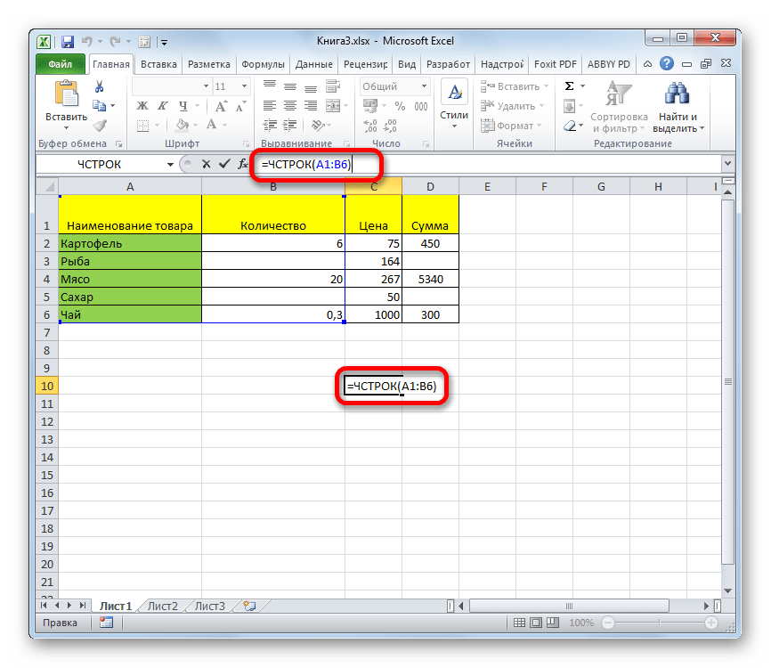
Для вывода результата на экран достаточно будет нажать кнопку Enter.

Причем подсчитываться будут даже полностью пустые строки диапазона. Стоит заметить, что в отличие от предыдущего способа, если вы выделите область, включающую несколько столбцов, то оператор будет считать исключительно строчки.

Пользователям, у которых небольшой опыт работы с формулами в Экселе, проще работать с данным оператором через Мастер функций.

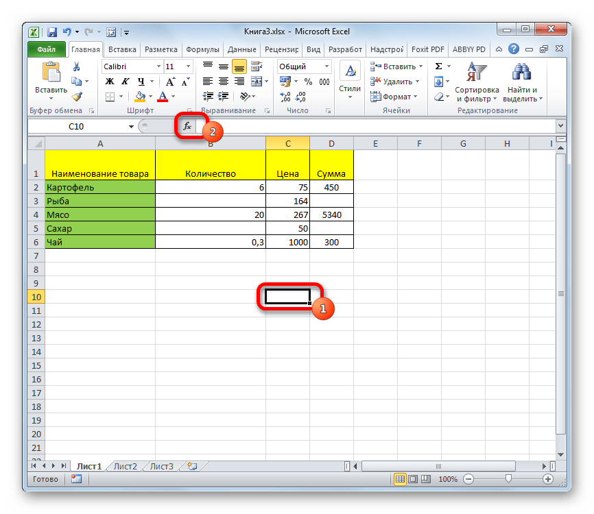
Выделяем ячейку, в которую будет производиться вывод готового итога подсчета элементов. Жмем на кнопку «Вставить функцию». Она размещена сразу слева от строки формул.

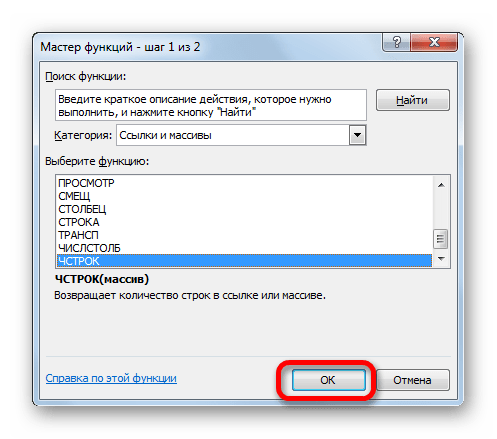
Запускается небольшое окно Мастера функций. В поле «Категории» устанавливаем позицию «Ссылки и массивы» или «Полный алфавитный перечень». Ищем значение «ЧСТРОК», выделяем его и жмем на кнопку «OK».

Открывается окно аргументов функции. Ставим курсор в поле «Массив». Выделяем на листе тот диапазон, количество строк в котором нужно подсчитать. После того, как координаты этой области отобразились в поле окна аргументов, жмем на кнопку «OK».

Программа обрабатывает данные и выводит результат подсчета строк в предварительно указанную ячейку. Теперь этот итог будет отображаться в данной области постоянно, если вы не решите удалить его вручную.

Урок: Мастер функций в Экселе

Способ 3: применение фильтра и условного форматирования

Но бывают случаи, когда нужно подсчитать не все строки диапазона, а только те, которые отвечают определенному заданному условию. В этом случае на помощь придет условное форматирование и последующая фильтрация

Выделяем диапазон, по которому будет производиться проверка на выполнение условия.

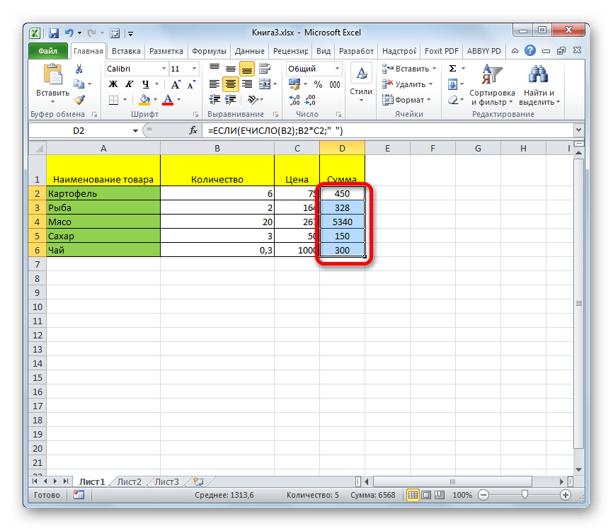
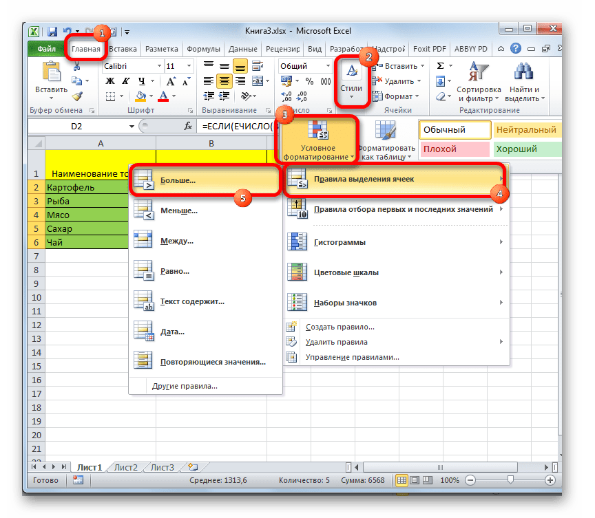
Переходим во вкладку «Главная». На ленте в блоке инструментов «Стили» жмем на кнопку «Условное форматирование». Выбираем пункт «Правила выделения ячеек». Далее открывается пункт различных правил. Для нашего примера мы выбираем пункт «Больше…», хотя для других случаев выбор может быть остановлен и на иной позиции.

Открывается окно, в котором задается условие. В левом поле укажем число, ячейки, включающие в себя значение больше которого, окрасятся определенным цветом. В правом поле существует возможность этот цвет выбрать, но можно и оставить его по умолчанию. После того, как установка условия завершена, жмем на кнопку «OK».

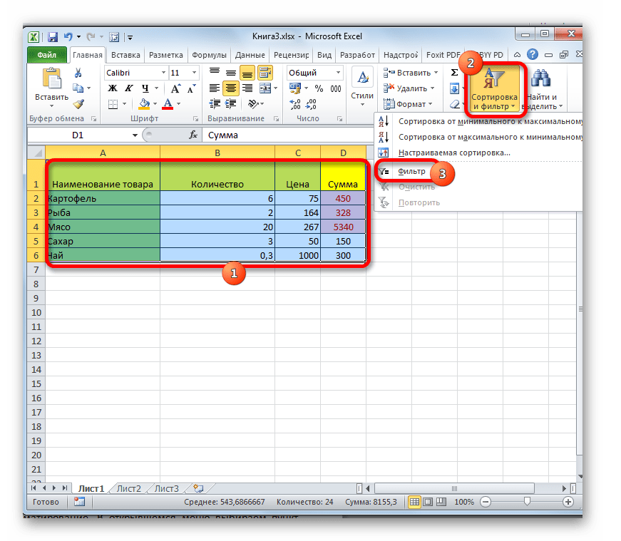
Как видим, после этих действий ячейки, удовлетворяющие условию, были залиты выбранным цветом. Выделяем весь диапазон значений. Находясь во все в той же вкладке «Главная», кликаем по кнопке «Сортировка и фильтр» в группе инструментов «Редактирование». В появившемся списке выбираем пункт «Фильтр».

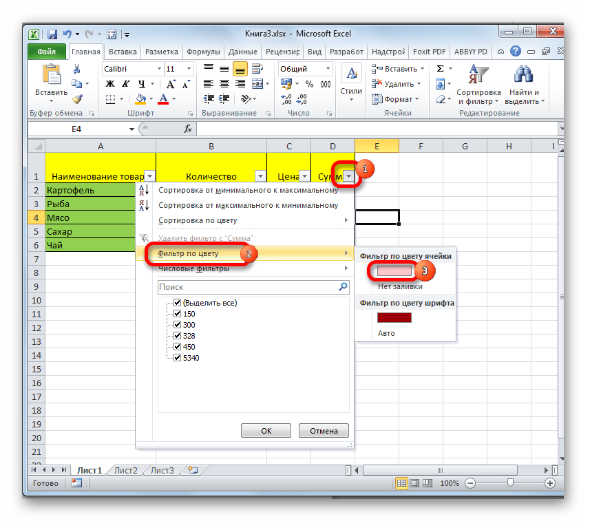
После этого в заглавиях столбцов появляется значок фильтра. Кликаем по нему в том столбце, где было проведено форматирование. В открывшемся меню выбираем пункт «Фильтр по цвету». Далее кликаем по тому цвету, которым залиты отформатированные ячейки, удовлетворяющие условию.

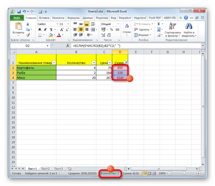
Как видим, не отмеченные цветом ячейки после данных действий были спрятаны. Просто выделяем оставшийся диапазон ячеек и смотрим на показатель «Количество» в строке состояния, как и при решении проблемы первым способом. Именно это число и будет указывать на численность строк, которые удовлетворяют конкретному условию.

Урок: Условное форматирование в Эксель

Урок: Сортировка и фильтрация данных в Excel

Как видим, существует несколько способов узнать количество строчек в выделенном фрагменте. Каждый из этих способов уместно применять для определенных целей. Например, если нужно зафиксировать результат, то в этом случае подойдет вариант с функцией, а если задача стоит подсчитать строки, отвечающие определенному условию, то тут на помощь придет условное форматирование с последующей фильтрацией.

Источник

I am trying to count the number of rows in a spreadsheet which contain at least one non-blank value over a few columns: i.e.

row 1 has a text value in column A
row 2 has a text value in column B
row 3 has a text value in column C
row 4 has no values in A, B or C

The formula would equate to 3, because rows 1, 2, & 3 have a text value in at least one column. Similarly if row 1 had a text value in each column (A, B, & C) this would be counted as 1.

ashleedawg

20k8 gold badges73 silver badges104 bronze badges

asked Jul 28, 2011 at 23:39

With formulas, what you can do is:

in a new column (say col D — cell D2), add =COUNTA(A2:C2)
drag this formula till the end of your data (say cell D4 in our example)
add a last formula to sum it up (e.g in cell D5): =SUM(D2:D4)

answered Jul 29, 2011 at 8:06

JMaxJMax

25.9k12 gold badges69 silver badges88 bronze badges

If you want a simple one liner that will do it all for you (assuming by no value you mean a blank cell):

=(ROWS(A:A) + ROWS(B:B) + ROWS(C:C)) - COUNTIF(A:C, "")

If by no value you mean the cell contains a 0

=(ROWS(A:A) + ROWS(B:B) + ROWS(C:C)) - COUNTIF(A:C, 0)

The formula works by first summing up all the rows that are in columns A, B, and C (if you need to count more rows, just increase the columns in the range. E.g. ROWS(A:A) + ROWS(B:B) + ROWS(C:C) + ROWS(D:D) + ... + ROWS(Z:Z)).

Then the formula counts the number of values in the same range that are blank (or 0 in the second example).

Last, the formula subtracts the total number of cells with no value from the total number of rows. This leaves you with the number of cells in each row that contain a value

TylerH

20.6k64 gold badges76 silver badges97 bronze badges

answered Dec 4, 2015 at 17:08

Jason McKindlyJason McKindly

4331 gold badge8 silver badges15 bronze badges

If you don’t mind VBA, here is a function that will do it for you. Your call would be something like:

=CountRows(1:10)

Function CountRows(ByVal range As range) As Long

Application.ScreenUpdating = False
Dim row As range
Dim count As Long

For Each row In range.Rows
    If (Application.WorksheetFunction.CountBlank(row)) - 256 <> 0 Then
        count = count + 1
    End If
Next

CountRows = count
Application.ScreenUpdating = True

End Function

How it works: I am exploiting the fact that there is a 256 row limit. The worksheet formula CountBlank will tell you how many cells in a row are blank. If the row has no cells with values, then it will be 256. So I just minus 256 and if it’s not 0 then I know there is a cell somewhere that has some value.

answered Jul 29, 2011 at 5:28

GaijinhunterGaijinhunter

14.5k4 gold badges50 silver badges57 bronze badges

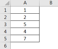
Try this scenario:

Array = A1:C7. A1-A3 have values, B2-B6 have value and C1, C3 and C6 have values.

To get a count of the number of rows add a column D (you can hide it after formulas are set up) and in D1 put formula =If(Sum(A1:C1)>0,1,0). Copy the formula from D1 through D7 (for others searching who are not excel literate, the numbers in the sum formula will change to the row you are on and this is fine).

Now in C8 make a sum formula that adds up the D column and the answer should be 6. For visually pleasing purposes hide column D.

JMax

25.9k12 gold badges69 silver badges88 bronze badges

answered Apr 29, 2012 at 18:15

You should use the sumif function in Excel:

=SUMIF(A5:C10;"Text_to_find";C5:C10)

This function takes a range like this square A5:C10 then you have some text to find this text can be in A or B then it will add the number from the C-row.

TylerH

20.6k64 gold badges76 silver badges97 bronze badges

answered Dec 13, 2012 at 11:08

This is what I finally came up with, which works great!

{=SUM(IF((ISTEXT('Worksheet Name!A:A))+(ISTEXT('CCSA Associates'!E:E)),1,0))-1}

Don’t forget since it is an array to type the formula above without the «{}», and to CTRL + SHIFT + ENTER instead of just ENTER for the «{}» to appear and for it to be entered properly.

TylerH

20.6k64 gold badges76 silver badges97 bronze badges

answered Oct 29, 2015 at 15:39

Источник

Need more help?

Need more help?

How to Count the Number of Rows in Excel?

Table of contents

#1 – Excel Count Rows which has only the Data

#2 – Count all the rows that have the data

#3 – Count the rows that only have the numbers

#4 – Count Rows, which only has the Blanks

#5 – Count rows that only have text values

#6 – Count all of the rows in the range

Things to Remember

Recommended Articles

Introduction to Row Count in Excel

How to Count the Rows in Excel?

Example #1

Example #2

Example #3

Example #4

Example #5

Example #6

Things to Remember About Row Count in Excel

Recommended Articles

Определение количества строк

Способ 1: указатель в строке состояния

Способ 2: использование функции

Способ 3: применение фильтра и условного форматирования