
Adding a color to alternate rows or columns (often called color banding) can make the data in your worksheet easier to scan. To format alternate rows or columns, you can quickly apply a preset table format. By using this method, alternate row or column shading is automatically applied when you add rows and columns.
Here’s how:
-
Select the range of cells that you want to format.
-
Click Home > Format as Table.
-
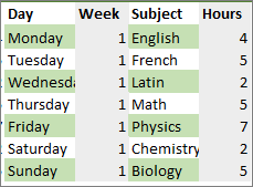
Pick a table style that has alternate row shading.
-
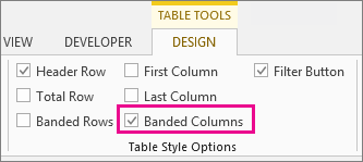
To change the shading from rows to columns, select the table, click Design, and then uncheck the Banded Rows box and check the Banded Columns box.

Tip: If you want to keep a banded table style without the table functionality, you can convert the table to a data range. Color banding won’t automatically continue as you add more rows or columns but you can copy alternate color formats to new rows by using Format Painter.
Use conditional formatting to apply banded rows or columns
You can also use a conditional formatting rule to apply different formatting to specific rows or columns.
Here’s how:
-
On the worksheet, do one of the following:
-
To apply the shading to a specific range of cells, select the cells you want to format.
-
To apply the shading to the whole worksheet, click the Select All button.
-
-
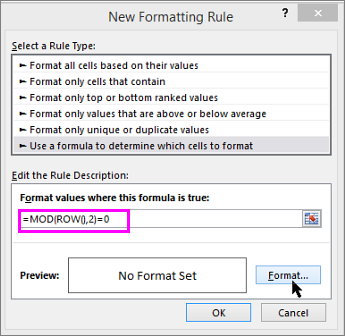
Click Home > Conditional Formatting > New Rule.
-
In the Select a Rule Type box, click Use a formula to determine which cells to format.
-
To apply color to alternate rows, in the Format values where this formula is true box, type the formula =MOD(ROW(),2)=0.
To apply color to alternate columns, type this formula: =MOD(COLUMN(),2)=0.
These formulas determine whether a row or column is even or odd numbered, and then applies the color accordingly.
-
Click Format.
-
In the Format Cells box, click Fill.
-
Pick a color and click OK.
-
You can preview your choice under Sample and click OK or pick another color.
Tips:
-
To edit the conditional formatting rule, click one of the cells that has the rule applied, click Home > Conditional Formatting > Manage Rules > Edit Rule, and then make your changes.
-
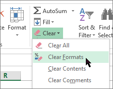
To clear conditional formatting from cells, select them, click Home > Clear, and pick Clear Formats.
-
To copy conditional formatting to other cells, click one of the cells that has the rule applied, click Home > Format Painter
, and then click the cells you want to format.
-
 , and then click the cells you want to format.
Need more help?
April 06, 2021/
Chris Newman
Implementing Row Banding (Alternating Colors)
While Excel does not have a dedicated row banding button to alternate row colors, there are a few creative ways we can obtain this effect. In this article we will walk through three solutions that will provide a way forward for how you might want to accomplish this:
-
Using an Excel Table
-
Using Conditional Formatting
-
Using a VBA Macro
Method 1: Utilize An Excel Table
An Excel Table is an object you can insert to allow for your data to be dynamically referenced throughout your spreadsheet. There are limitations that come with the Table object (such as every column has to have a unique heading), but if you can live with some of the restrictions, this is a great way to alternate row colors automatically.
Converting your spreadsheet range to a table object is as easy as
-
Select your data range
-
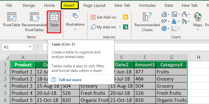
Navigate to the Insert Tab on your Ribbon Menu
-
Click the Table Button
-
Tell the dialog box if your selection included headers
-
Click OK
Alternatively, you can select your data range and use the keyboard shortcut Ctrl + t to get to the insert Table dialog box.
If you do not like one of the default Table Style options, you can create your own Table format to get specific row colors. Just click New Table Style at the very bottom of the Table Styles gallery in Excel Ribbon.
Method 2: Conditional Formatting
If you don’t want to utilize an Excel table, you can alternatively utilize conditional formatting rules to get alternating colors.
The only disadvantage to this method is you (as of this writing) cannot reference named ranges in conditional formatting rules. This means if you add a new row to the bottom of the table at a later date, you will need to update the conditional formatting data range to ensure the new row is included in the rule.
Note: If you insert a row inside your currently formatted rows, the conditional formatting rule will automatically adjust to include it.
To create this color banding, you will need to select the cell range you are targeting and add a new Conditional Formatting rule.
-
Navigate to the Home Tab
-
Click the Conditional Formatting menu button
-
Select New Rule…
-
In the New Formatting Rule dialog box, select “Use a formula to determine which cells to format”
-
Enter one of the MOD functional rules noted below:
-
For even-numbered rows, you’ll want to use one of the following formulas:
-
=ISEVEN(ROW())
-
=MOD(ROW(),2)=0
-
-
For odd-numbered rows, you’ll want to use one of the following formulas:
-
=ISODD(ROW())
-
=MOD(ROW(),2)>0
-
-
-
Click the Format Button and select the specific formatting you wish to apply (I just chose a fill color of gray)
-
Click OK Button
-
Repeat steps 1-7 for the secondary color
Once you’ve created both your primary and secondary banding conditional formatting rules, you should see the alternating colors automatically apply.
Method 3: VBA Coded Macro
Maybe you are looking for a solution that is more ad-hoc or on-demand. For times where you want to quickly format a table before sending it off to the executives, having a personal macro that can band your data in a pinch might be the right answer for your needs.
The below code allows you to select a range on your spreadsheet and quickly alternate two different colors across the rows. Just programmatically define the two color codes you wish to use (you can reference VB colors or an RGB color code for more flexibility/variety) at the beginning of the code.
The remaining VBA code loops through each row and alternates the fill colors applied based on odd/even rows. If you would like to learn a bit more about the technique used to determine odd/even rows, you can check out this article: VBA To Determine If Number Is Odd Or Even.
Sub AlternateRowColors()
‘PURPOSE: Alternate row fill colors based on selected range
‘SOURCE: www.TheSpreadsheetGuru.com/the-code-vault
Dim rng As Range
Dim x As Long
Dim LightColorCode As Long
Dim DarkColorCode As Long
‘Define Colors (Input)
LightColorCode = vbWhite
DarkColorCode = RGB(242, 242, 242)
‘Ensure a Range is Selected
If TypeName(Selection) <> «Range» Then Exit Sub
‘Store Selected range to a variable
Set rng = Selection
‘Check for more than 1 row selected
If rng.Rows.Count = 1 Then Exit Sub
‘Loop through each row in selection and color appropriately
For x = 1 To rng.Rows.Count
If x Mod 2 = 0 Then
rng.Rows(x).Interior.Color = DarkColorCode ‘Even Row
Else
rng.Rows(x).Interior.Color = LightColorCode ‘Odd Row
End If
Next x
End Sub
Download The Excel Example File
If you would like to get a copy of the Excel file I used throughout this article, feel free to directly download the spreadsheet by clicking the download button below.
I Hope This Helped!
Hopefully, I was able to explain how you can use a number of different methods in Excel to alternate row colors in a given cell range. If you have any questions about these techniques or suggestions on how to improve them, please let me know in the comments section below.
About The Author
Hey there! I’m Chris and I run TheSpreadsheetGuru website in my spare time. By day, I’m actually a finance professional who relies on Microsoft Excel quite heavily in the corporate world. I love taking the things I learn in the “real world” and sharing them with everyone here on this site so that you too can become a spreadsheet guru at your company.
Through my years in the corporate world, I’ve been able to pick up on opportunities to make working with Excel better and have built a variety of Excel add-ins, from inserting tickmark symbols to automating copy/pasting from Excel to PowerPoint. If you’d like to keep up to date with the latest Excel news and directly get emailed the most meaningful Excel tips I’ve learned over the years, you can sign up for my free newsletters. I hope I was able to provide you some value today and hope to see you back here soon! — Chris
How to Add Alternate Row Color in Excel?
Below mentioned are the two different methods to add color to alternative rows:
- Add alternative row colors using Excel table styles
- Highlight alternative rows using Excel “Conditional Formatting” option
Now, let us discuss each method in detail with an example.
Table of contents
- How to Add Alternate Row Color in Excel?
- #1 Add Alternative Row Color Using Excel Table Styles
- #2 Highlight Alternate Row Color using Excel Conditional Formatting
- Benefits of using Excel Alternate Row Colors
- Things to Remember
- Recommended Articles
#1 Add Alternative Row Color Using Excel Table Styles
The quickest and most straightforward approach to apply row shading in Excel is by utilizing predefined.
- First, we must select the data or range where we want to add the color in a row.

- Then, click on the “Insert” tab on the Excel ribbon and click “Table” to choose the function.

- When we click on the “Table,” the dialog box will select the range.

- Click on the “OK.” Now, we will get the table with alternate row colors in Excel, as shown below:

- Suppose we do not want the table with rows. We would preferably have alternate column shading just without the table usefulness. We can undoubtedly change over the table back to a standard range. We need to select any cell inside the table, right-click and choose “Convert to Range” from the setting menu.

- Then, select the table or data, and go to the “Design” tab.

- Next, we need to go to table style and choose the color of the table which is required and selected by us.


#2 Highlight Alternate Row Color using Excel Conditional Formatting
- Step 1: First, we need to select the data or range in the Excel sheet.
- Step 2: Go to the “Home” tab and “Styles” group, and click on conditional formatting in the ExcelConditional formatting is a technique in Excel that allows us to format cells in a worksheet based on certain conditions. It can be found in the styles section of the Home tab.read more ribbon.

- Step 3: Choose a “New Rule” from the drop-down list in excelA drop-down list in excel is a pre-defined list of inputs that allows users to select an option.read more:

- Step 4: In the “New Formatting Rule” dialog box, we must choose the option at the bottom of the dialog box, “Use a formula to determine which cells to format,” and insert the following formula in a tab to get the result
- =MOD(ROW(),2)=0

- Step 5: Click the “Format” button on the right-hand side, click on the switch to the “Fill” tab, and choose the background color we want to use or required for the banded rows in the Excel sheet.

- Step 6: In the dialog box, as shown above, the color we have selected will appear under the “Sample” at the bottom of the dialog box. If we are satisfied with the color, click “OK” to choose the same color, which shows in a sample.
- Step 7: Once we click on “OK,” it will carry us back to the “New Formatting Rule” window in the Excel sheet, and when you click “OK” again, apply the Excel color to the alternate row of the certain rows. Click “OK.” We will get the alternate row color in Excel with yellow color, as shown below.
Benefits of using Excel Alternate Row Colors
- To improve the readability of the Excel sheet, some users shade every other row in a huge Excel sheet.
- Colors can enable us to envision our information adequately by empowering us to perceive gatherings of related data by sight.
- When we use the color in your spreadsheet, this theory makes the difference.
- Adding shading to alternate rows or columns (which is called shading banding) can make the information in our worksheet less demanding to examine.
- If any rows are inserted or deleted from the row shading, it automatically adjusts to maintain our table’s pattern.
Things to Remember
- We must always use decent colors while coloring the alternate color because the bright color cannot solve our purpose.
- While using the conditional formula, we must always enter the formula in the tab. Otherwise, we will not be able to color the row.
- We should use dark colors for the text to easily read the data in the Excel worksheet.
- If we want to print your excel sheetThe print feature in excel is used to print a sheet or any data. While we can print the entire worksheet at once, we also have the option of printing only a portion of it or a specific table.read more, we must ensure that we use a light or decent color shade to highlight the rows to read it very easily.
- We must try not to use the excess conditional formatting function in our data because it creates confusion.
Recommended Articles
This article has been a guide to Excel Alternate Row Color. We discuss adding color to alternate rows using table style and conditional formatting, examples, and a downloadable Excel template. You may learn more about Excel from the following articles: –
- Excel Sum by Color
- Sort by Color in Excel
- Use Dynamic Tables in Excel
- How to use Excel Tables?
Reader Interactions
Introduction
It is just a common training to add color to alternate rows within an Excel Spreadsheet to make it simpler and to enhance readability. In a spreadsheet, if you will find several rows to be colored, and you have to do it one by one, it will soon be time-consuming and tiring as well. One of the greatest methods to make points clearer is to color every switch row in the sheet. The feature applies to MS Excel 2007 and higher versions.
This article describes how to highlight every other row in excel. You can quickly color every other row in Excel, as there are different rows or columns in your spreadsheet. Please check out the two probable techniques below…
How Excel highlight Every Other Row by Using the “Format as Table” option
- On a new spreadsheet, choose the cell range that you want to color the alternate row, or press Ctrl + A to choose the whole data. For example, I have selected a variety of data from F5 to H13. Please browse the screenshot.

2. Under the Home tab, locate the styles group and click Format as Table. In addition, you can use the arrow buttons to scroll through the available table styles to view them all and to check everything is insured and bonded. In the example below, I’ve selected table style.
3. And finally, your selected data will have alternate colors in a row. Please see the result.

Use the “Conditional Formatting” option to color every other row in excel
- Initially, open an Excel file or input specific data on your new spreadsheet. And Select the cell range that you wish to shade, or press Ctrl + A to select the complete data. In the example, I have the exact same data as explained in the previous method.
- Next, Under the Home tab, find the Styles group, and click Conditional Formatting, and then select New Rule… options. Please start to see the screenshot below:

3. On a New Formatting Rule window, select Use a formula to determine which cells to format. In the Format values where this formula is just a true input box, type the formula = MOD (ROW (), 2) = 1 manually and then click Format open, Format Cells dialog box.
tips:
- Here I use the formula = MOD (ROW (), 2) = 1 to color the odd rows. If you wish to color the even rows try a formula like this, = MOD (ROW (), 2) = 0.
- If you wish to color alternate columns instead of alternate rows you can use the exact same formula. Only change ROW () purpose by COLUMN () function. Please try to find the difference!

4. Then on the Format Cells dialog box, click the Fill tab, and select the color that you want to use to color every other row, and then click OK. This will be a preview of the filled color for your previous New Formatting Rule window. Click OK to close the New Formatting Rule dialog box.

5. And finally your result will be as:

Conclusion
That is all about the excel alternate row color. Easy and exciting, right? Do practice these tricks as you already know that practice makes a man perfect! Thank you for reading!
Alternate Row Color Excel (Table of Contents)
- Introduction to Excel Alternate Row Color
- How to Add Alternate Row Color in Excel?
Introduction to Excel Alternate Row Color
In Microsoft excel, “Alternate Row Color” is mostly used in a table to display their data more accurate. Most of the organization needs to present their data in a professional manner. Applying alternate color and unique color to the data is to make the sheets more perfect which makes the data to view it in a colorful format. In Microsoft Excel, we can either apply color to the rows manually or by simply formatting the row so that we can apply the color shading to the specific rows and columns.
How to Add Alternate Row Color in Excel?
To add Alternate Row Color in Excel is very simple and easy. Let’s understand how to add Alternate Row Color with some examples.
You can download this Alternate Row Color Excel Template here – Alternate Row Color Excel Template
In excel, we can apply color to the rows manually by selecting a unique color to the rows. Selecting an alternate color makes it a difficult task for the users. In order to overcome these things excel has given us a formatting table option where we can select a wide range of alternate row colors for the table. Let’s look at a few examples.
Example #1 – Formatting Row Table
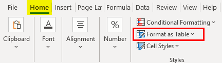
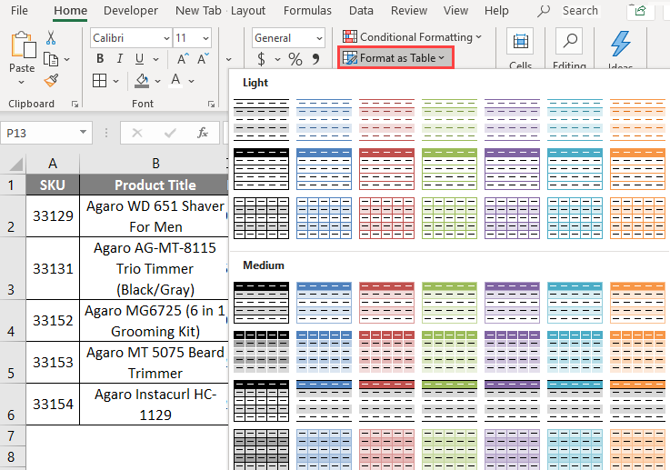
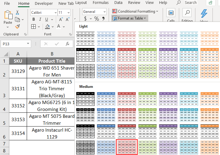
We can find the formatting tables in Microsoft Excel in the HOME menu under the STYLES group, which is shown below.
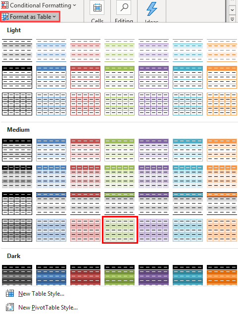
Once we click on the format table, we can find various table styles with alternate row colors, which are shown below.
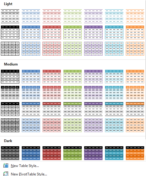
In the above screenshot, we can see that there are various table styles that come with the option like Light, Medium, and Dark.
For example, if we wish to apply a different color to the row, we can simply click the format table and choose any one of the colors that we need to apply.
Example #2 – Applying Alternate Color to the Rows
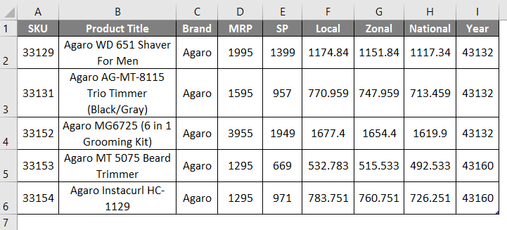
In this example, we will learn how to apply alternate colors to the row by using the below data. Consider the below example where we have some sales data table with no fill color.
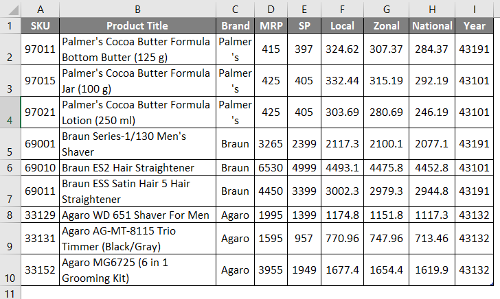
Assume that we need to apply alternate colors to the row, which makes the data more colorful.
We can apply alternate color to the rows by following the below steps as follows:
First, go to the format table option in the Styles group. Click on the format as table down arrow so that we will get various table styles as shown below.
Select the row table color to fill it.
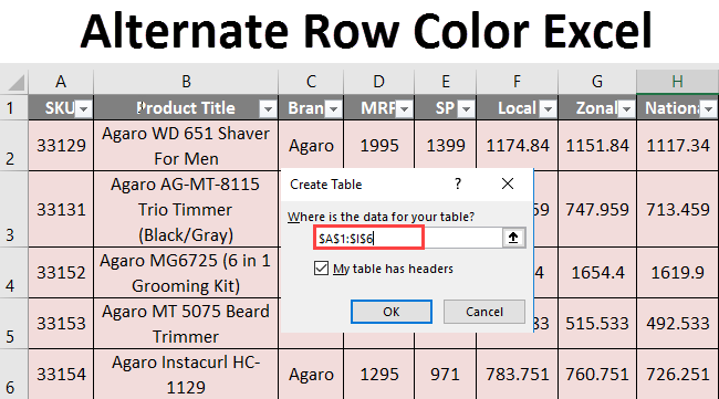
Here in this example, we will choose “TABEL STYLE MEDIUM 25”, which shows a combination of dark and light green which is shown in the below screenshot.
Once we click on that MEDIUM table style, we will get the below format table dialog box which is shown below.
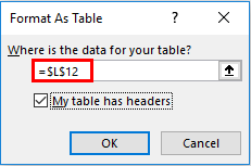
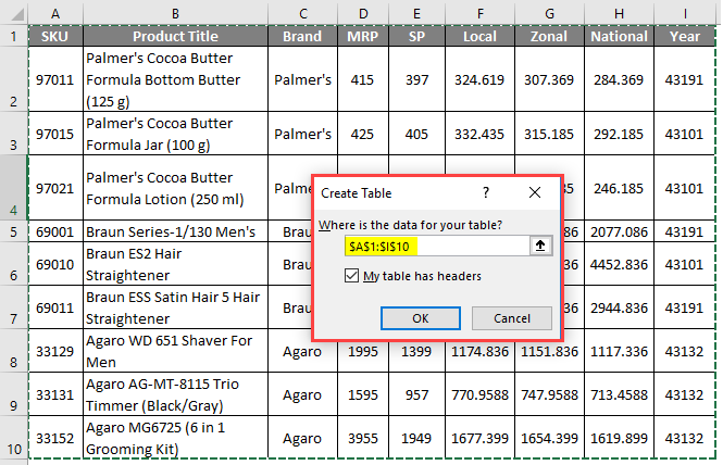
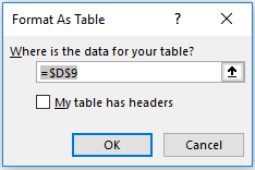
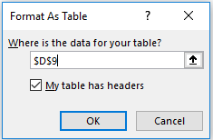
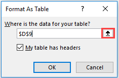
Now, checkmark the “My table HAS HEADERS” because our sales data has already had headers named as SKU, Product title, etc. Next, we need to select the range selection for the table. Click on the red arrow mark as shown below.
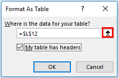
Once we click on the red arrow, we will get the selection range which is shown below.
Result
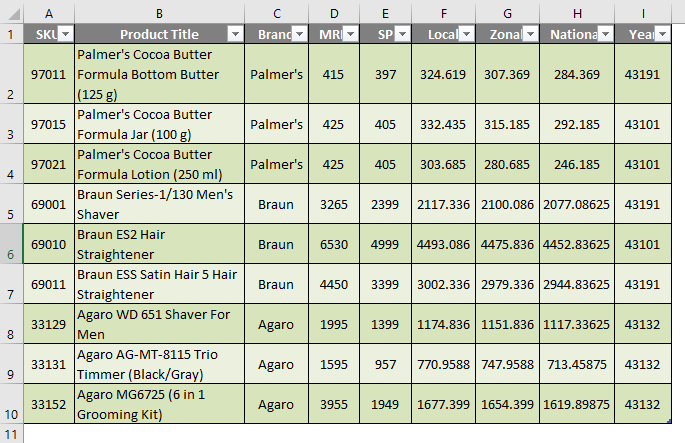
We can see that each row has been filled with different alternate row colors in the below result, making the data a perfect view.
Example #3 – Applying Alternate Row Colors using Banding
In Microsoft Excel, applying alternate colors is also called Banding, where we have the option while doing table formatting. In this example, we will see how to apply alternate colors to rows using Banding by following the below steps as follows. Consider the below example, which has sales data without formatting.
Now we can apply the banding option by using the format table by following the below steps. First, go to the format table option in the Styles group. Click on the format as table down arrow so that we will get the various table styles which are shown below.
Select the row table color to fill it.
Here in this example, we will choose “TABEL STYLE – MEDIUM 24”, which shows a combination of dark and light green which is shown in the below screenshot.
Once we click on that MEDIUM table style, we will get the below format table dialog box which is shown below.
Now, checkmark the “My table has headers” because our sales data already has headers named as SKU, Product title, etc.
Next, we need to select the range selection for the table. Click on the red arrow mark as shown below.
Once we click on the red arrow, we will get the selection range which is shown below. Select the table range from A1 to I6, which is shown in the below screenshot.
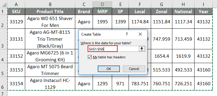
After selecting the range for the table, make sure that “My table has the header” is enabled. Click Ok so that we will get the below result as follows.
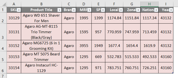
Now we can see that each row has been filled with alternate color. We can make the row shading by enabling the option called Banding Rows by following the below steps. Select the above-formatted table so that we will get the design menu which is shown in the below screenshot.
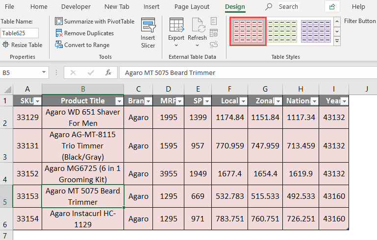
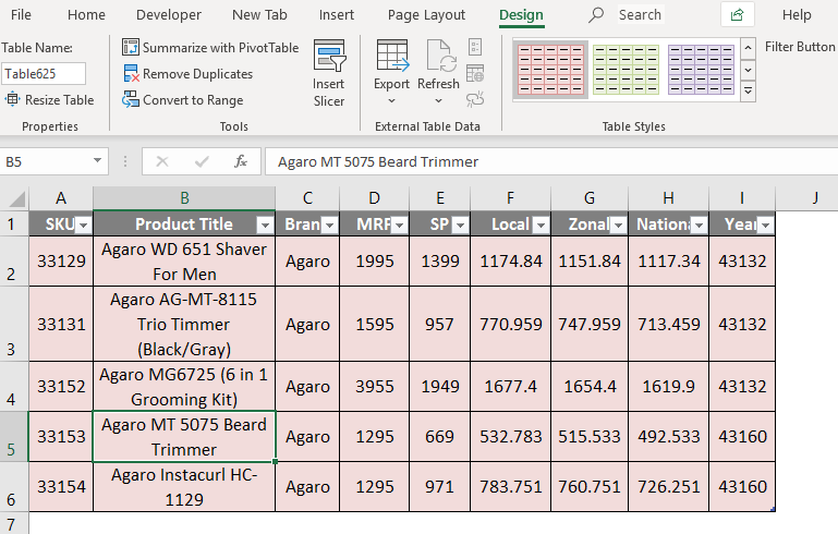
In the design menu, we can notice that “Banded Row” is already enabled, and for that reason, we are getting the shaded row color. We can disable the Banded row by removing the checkmark, which is shown in the below screenshot. Once we remove the checkmark for Banded rows, the dark pink color will be removed, shown below.
Results
In the below result, we can notice that the row color has been changed to light pink because of the removal of Banded Rows.
Example #4 – Applying Alternate Row Color using Conditional Formatting
In this example, we will see how to apply alternate row colors by using conditional formatting. Consider the below example, which has sales raw data with no row color, which is shown below.
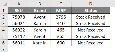
We can apply conditional formatting to display alternate row colors by following the below step. First, select the Brand row to apply the Alternate color for rows which is shown in the below screenshot.
Next, go to conditional formatting and choose “Highlight Cells Rules”, where we will get an option called “Text That Contains”, which is shown below.
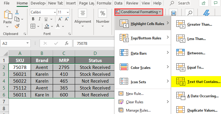
Click on the “TEXT THAT CONTAIN” option so that we will get the below dialog box.
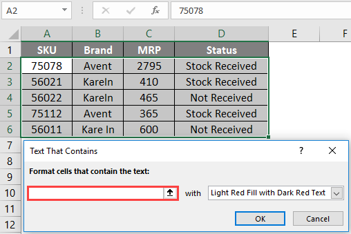
Now in the dialog box, give the text name on the right-hand side, and we can see the drop-down box on the left-hand side where we can choose text color for highlighting. Here in this example, give the text name as Avent and choose the “Green fill with Dark Green Text” shown below.
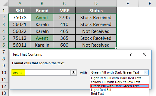
Once we select the Highlight text color, click on Ok
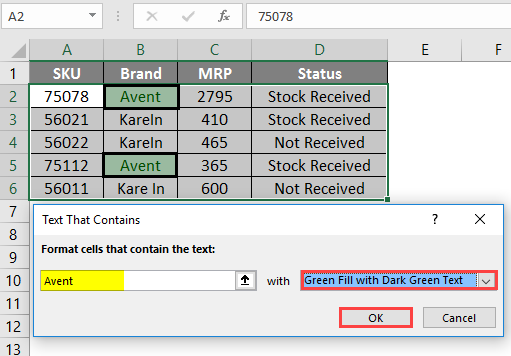
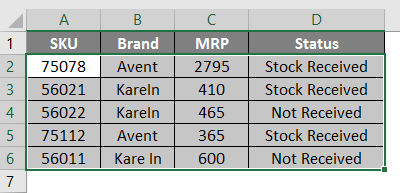
Once we click on ok will get the below output as follows.
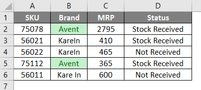
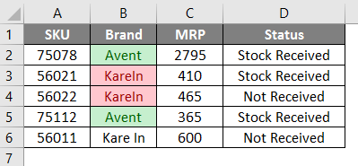
Apply the same for other brand names so that we will get the final output as shown below.
Result
In the below result, we can see that alternate row color has been applied using conditional formatting.
Things to Remember About Alternate Row Color Excel
- We can apply an alternate row color only to the preset tables either by formatting the table or using conditional formatting.
- While formatting the table, make sure that we header is enabled or else excel will overwrite the headers we have mentioned.
Recommended Articles
This is a guide to Alternate Row Color Excel. Here we have discussed How to add Alternate Row Color Excel along with practical examples and a downloadable excel template. You can also go through our other suggested articles –
- Color in Excel
- Shade Alternate Rows in Excel
- VBA Color Index
- ROWS Function in Excel