
If you find yourself needing to expand or reduce Excel’s row widths and column heights, there are several ways to adjust them. The table below shows the minimum, maximum and default sizes for each based on a point scale.
|
Type |
Min |
Max |
Default |
|---|---|---|---|
|
Column |
0 (hidden) |
255 |
8.43 |
|
Row |
0 (hidden) |
409 |
15.00 |
Notes:
-
If you are working in Page Layout view (View tab, Workbook Views group, Page Layout button), you can specify a column width or row height in inches, centimeters and millimeters. The measurement unit is in inches by default. Go to File > Options > Advanced > Display > select an option from the Ruler Units list. If you switch to Normal view, then column widths and row heights will be displayed in points.
-
Individual rows and columns can only have one setting. For example, a single column can have a 25 point width, but it can’t be 25 points wide for one row, and 10 points for another.

Set a column to a specific width
-
Select the column or columns that you want to change.
-
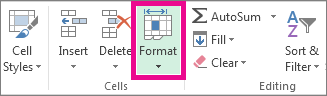
On the Home tab, in the Cells group, click Format.

-
Under Cell Size, click Column Width.
-
In the Column width box, type the value that you want.
-
Click OK.
Tip: To quickly set the width of a single column, right-click the selected column, click Column Width, type the value that you want, and then click OK.
-
Select the column or columns that you want to change.
-
On the Home tab, in the Cells group, click Format.
-
Under Cell Size, click AutoFit Column Width.
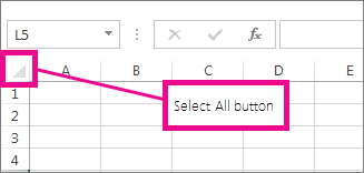
Note: To quickly autofit all columns on the worksheet, click the Select All button, and then double-click any boundary between two column headings.
-
Select a cell in the column that has the width that you want to use.
-
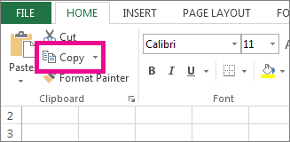
Press Ctrl+C, or on the Home tab, in the Clipboard group, click Copy.
-
Right-click a cell in the target column, point to Paste Special, and then click the Keep Source Columns Widths
button.
 button.
The value for the default column width indicates the average number of characters of the standard font that fit in a cell. You can specify a different number for the default column width for a worksheet or workbook.
-
Do one of the following:
-
To change the default column width for a worksheet, click its sheet tab.
-
To change the default column width for the entire workbook, right-click a sheet tab, and then click Select All Sheets on the shortcut menu.
-
-
On the Home tab, in the Cells group, click Format.
-
Under Cell Size, click Default Width.
-
In the Standard column width box, type a new measurement, and then click OK.

Do one of the following:
-
To change the width of one column, drag the boundary on the right side of the column heading until the column is the width that you want.
-
To change the width of multiple columns, select the columns that you want to change, and then drag a boundary to the right of a selected column heading.
-
To change the width of columns to fit the contents, select the column or columns that you want to change, and then double-click the boundary to the right of a selected column heading.
-
To change the width of all columns on the worksheet, click the Select All button, and then drag the boundary of any column heading.
-
Select the row or rows that you want to change.
-
On the Home tab, in the Cells group, click Format.
-
Under Cell Size, click Row Height.
-
In the Row height box, type the value that you want, and then click OK.
-
Select the row or rows that you want to change.
-
On the Home tab, in the Cells group, click Format.
-
Under Cell Size, click AutoFit Row Height.
Tip: To quickly autofit all rows on the worksheet, click the Select All button, and then double-click the boundary below one of the row headings.
Do one of the following:
-
To change the row height of one row, drag the boundary below the row heading until the row is the height that you want.
-
To change the row height of multiple rows, select the rows that you want to change, and then drag the boundary below one of the selected row headings.
-
To change the row height for all rows on the worksheet, click the Select All button, and then drag the boundary below any row heading.
-
To change the row height to fit the contents, double-click the boundary below the row heading.
Top of Page
If you prefer to work with column widths and row heights in inches, you should work in Page Layout view (View tab, Workbook Views group, Page Layout button). In Page Layout view, you can specify a column width or row height in inches. In this view, inches are the measurement unit by default, but you can change the measurement unit to centimeters or millimeters.
-
In Excel 2007, click the Microsoft Office Button
> Excel Options> Advanced. -
In Excel 2010, go to File > Options > Advanced.
 > Excel Options> Advanced.
Set a column to a specific width
-
Select the column or columns that you want to change.
-
On the Home tab, in the Cells group, click Format.
-
Under Cell Size, click Column Width.
-
In the Column width box, type the value that you want.

-
Select the column or columns that you want to change.
-
On the Home tab, in the Cells group, click Format.
-
Under Cell Size, click AutoFit Column Width.
Tip To quickly autofit all columns on the worksheet, click the Select All button and then double-click any boundary between two column headings.

-
Select a cell in the column that has the width that you want to use.
-
On the Home tab, in the Clipboard group, click Copy, and then select the target column.
-
On the Home tab, in the Clipboard group, click the arrow below Paste, and then click Paste Special.
-
Under Paste, select Column widths.

The value for the default column width indicates the average number of characters of the standard font that fit in a cell. You can specify a different number for the default column width for a worksheet or workbook.
-
Do one of the following:
-
To change the default column width for a worksheet, click its sheet tab.
-
To change the default column width for the entire workbook, right-click a sheet tab, and then click Select All Sheets on the shortcut menu.
-
-
On the Home tab, in the Cells group, click Format.
-
Under Cell Size, click Default Width.
-
In the Default column width box, type a new measurement.

Tip If you want to define the default column width for all new workbooks and worksheets, you can create a workbook template or a worksheet template, and then base new workbooks or worksheets on those templates. For more information, see Save a workbook or worksheet as a template.
Do one of the following:
-
To change the width of one column, drag the boundary on the right side of the column heading until the column is the width that you want.
-
To change the width of multiple columns, select the columns that you want to change, and then drag a boundary to the right of a selected column heading.
-
To change the width of columns to fit the contents, select the column or columns that you want to change, and then double-click the boundary to the right of a selected column heading.
-
To change the width of all columns on the worksheet, click the Select All button, and then drag the boundary of any column heading.
-
Select the row or rows that you want to change.
-
On the Home tab, in the Cells group, click Format.
-
Under Cell Size, click Row Height.
-
In the Row height box, type the value that you want.
-
Select the row or rows that you want to change.
-
On the Home tab, in the Cells group, click Format.
-
Under Cell Size, click AutoFit Row Height.
Tip To quickly autofit all rows on the worksheet, click the Select All button and then double-click the boundary below one of the row headings.
Do one of the following:
-
To change the row height of one row, drag the boundary below the row heading until the row is the height that you want.
-
To change the row height of multiple rows, select the rows that you want to change, and then drag the boundary below one of the selected row headings.
-
To change the row height for all rows on the worksheet, click the Select All button, and then drag the boundary below any row heading.
-
To change the row height to fit the contents, double-click the boundary below the row heading.
Top of Page
See Also
Change the column width or row height (PC)
Change the column width or row height (Mac)
Change the column width or row height (web)
How to avoid broken formulas
Do you have some values arranged as rows in your workbook, and do you want to convert text in rows to columns in Excel like this?
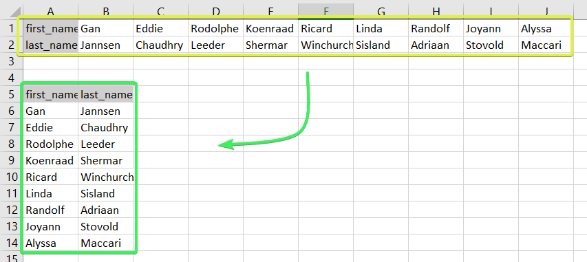
In Excel, you can do this manually or automatically in multiple ways depending on your purpose. Read on to get all the details and choose the best solution for yourself.
How to convert rows into columns or columns to rows in Excel – the basic solution
The easiest way to convert rows to columns in Excel is via the Paste Transpose option. Here is how it looks:
- Select and copy the needed range
- Right-click on a cell where you want to convert rows to columns
- Select the Paste Transpose option to rotate rows to columns
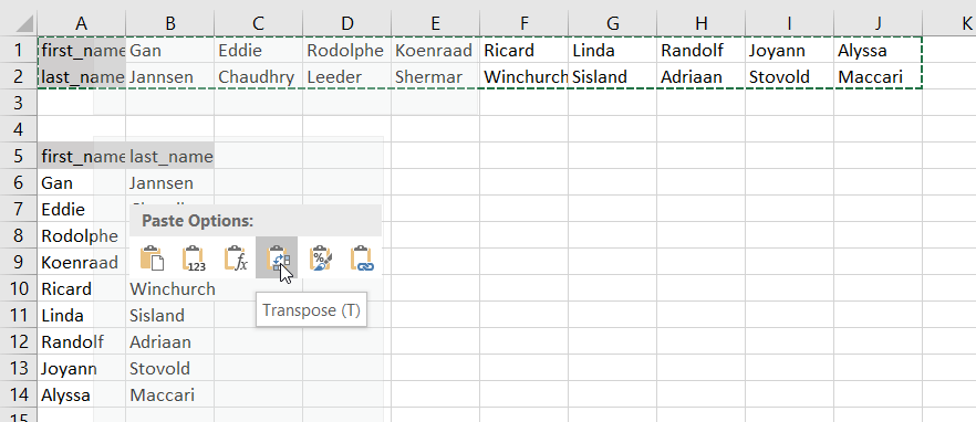
As an alternative, you can use the Paste Special option and mark Transpose using its menu.

It works the same if you need to convert columns to rows in Excel.

This is the best way for a one-time conversion of small to medium numbers of rows both in the Excel desktop and online.
Can I convert multiple rows to columns in Excel from another workbook?
The method above will work well if you want to convert rows to columns in Excel between different workbooks using Excel desktop. You need to have both spreadsheets open and do the copying and pasting as described.
However, in Excel Online, this won’t work for different workbooks. The Paste Transpose option is not available.
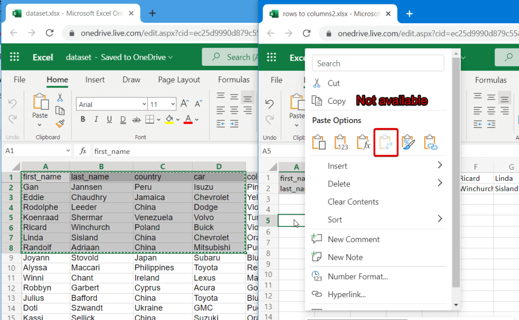
Therefore, in this case, it’s better to use the TRANSPOSE function.
How to switch rows and columns in Excel in more efficient ways
To switch rows and columns in Excel automatically or dynamically, you can use one of these options:
- Excel TRANSPOSE function
- VBA macro
- Power Query
Let’s check out each of them in the example of a data range that we imported to Excel from a Google Sheets file using Coupler.io.

Coupler.io is an integration solution that synchronizes data between source and destination apps on a regular schedule. For example, you can set up an automatic data export from Google Sheets every day to your Excel workbook.
Check out all the available Excel integrations.

How to change row to column in Excel with TRANSPOSE
TRANSPOSE is the Excel function that allows you to switch rows and columns in Excel. Here is its syntax:
=TRANSPOSE(array)array– an array of columns or rows to transpose
One of the main benefits of TRANSPOSE is that it links the converted columns/rows with the source rows/columns. So, if the values in the rows change, the same changes will be made in the converted columns.
TRANSPOSE formula to convert multiple rows to columns in Excel desktop
TRANSPOSE is an array formula, which means that you’ll need to select a number of cells in the columns that correspond to the number of cells in the rows to be converted and press Ctrl+Shift+Enter.
=TRANSPOSE(A1:J2)
Fortunately, you don’t have to go through this procedure in Excel Online.
TRANSPOSE formula to rotate row to column in Excel Online
You can simply insert your TRANSPOSE formula in a cell and hit enter. The rows will be rotated to columns right away without any additional button combinations.

Excel TRANSPOSE multiple rows in a group to columns between different workbooks
We promised to demonstrate how you can use TRANSPOSE to rotate rows to columns between different workbooks. In Excel Online, you need to do the following:
- Copy a range of columns to rotate from one spreadsheet and paste it as a link to another spreadsheet.

- We need this URL path to use in the TRANSPOSE formula, so copy it.

- The URL path above is for a cell, not for an array. So, you’ll need to slightly update it to an array to use in your TRANSPOSE formula. Here is what it should look like:
=TRANSPOSE('https://d.docs.live.net/ec25d9990d879c55/Docs/Convert rows to columns/[dataset.xlsx]dataset'!A1:D12)

You can follow the same logic for rotating rows to columns between workbooks in Excel desktop.
Are there other formulas to convert columns to rows in Excel?
TRANSPOSE is not the only function you can use to change rows to columns in Excel. A combination of INDIRECT and ADDRESS functions can be considered as an alternative, but the flow to convert rows to columns in Excel using this formula is much trickier. Let’s check it out in the following example.
How to convert text in columns to rows in Excel using INDIRECT+ADDRESS
If you have a set of columns with the first cell A1, the following formula will allow you to convert columns to rows in Excel.
=INDIRECT(ADDRESS(COLUMN(A1),ROW(A1)))

But where are the rows, you may ask! Well, first you need to drag this formula down if you are converting multiple columns to rows. Then drag it to the right.

NOTE: This Excel formula only to convert data in columns to rows starting with A1 cell. If your columns start from another cell, check out the next section.
How to convert Excel data in columns to rows using INDIRECT+ADDRESS from other cells
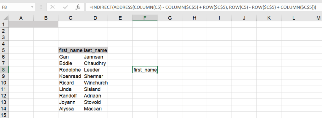
To convert columns to rows in Excel with INDIRECT+ADDRESS formulas from not A1 cell only, use the following formula:
=INDIRECT(ADDRESS(COLUMN(first_cell) - COLUMN($first_cell) + ROW($first_cell), ROW(first_cell) - ROW($first_cell) + COLUMN($first_cell)))
- first_cell – enter the first cell of your columns
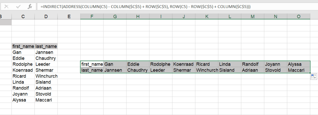
Here is an example of how to convert Excel data in columns to rows:
=INDIRECT(ADDRESS(COLUMN(C5) - COLUMN($C$5) + ROW($C$5), ROW(C5) - ROW($C$5) + COLUMN($C$5)))
Again, you’ll need to drag the formula down and to the right to populate the rest of the cells.
How to automatically convert rows to columns in Excel VBA
VBA is a superb option if you want to customize some function or functionality. However, this option is only code-based. Below we provide a script that allows you to change rows to columns in Excel automatically.
- Go to the Visual Basic Editor (VBE). Click Alt+F11 or you can go to the Developer tab => Visual Basic.

- In VBE, go to Insert => Module.
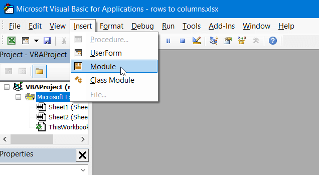
- Copy and paste the script into the window. You’ll find the script in the next section.

- Now you can close the VBE. Go to Developer => Macros and you’ll see your RowsToColumns macro. Click Run.

- You’ll be asked to select the array to rotate and the cell to insert the rotated columns.

- There you go!

VBA macro script to convert multiple rows to columns in Excel
Sub TransposeColumnsRows()
    Dim SourceRange As Range
    Dim DestRange As Range

    Set SourceRange = Application.InputBox(Prompt:="Please select the range to transpose", Title:="Transpose Rows to Columns", Type:=8)
    Set DestRange = Application.InputBox(Prompt:="Select the upper left cell of the destination range", Title:="Transpose Rows to Columns", Type:=8)

    SourceRange.Copy
    DestRange.Select
    Selection.PasteSpecial Paste:=xlPasteAll, Operation:=xlNone, SkipBlanks:=False, Transpose:=True
    Application.CutCopyMode = False

End Sub

Sub RowsToColumns()
    Dim SourceRange As Range
    Dim DestRange As Range

    Set SourceRange = Application.InputBox(Prompt:="Select the array to rotate", Title:="Convert Rows to Columns", Type:=8)
    Set DestRange = Application.InputBox(Prompt:="Select the cell to insert the rotated columns", Title:="Convert Rows to Columns", Type:=8)

    SourceRange.Copy
    DestRange.Select
    Selection.PasteSpecial Paste:=xlPasteAll, Operation:=xlNone, SkipBlanks:=False, Transpose:=True
    Application.CutCopyMode = False

End Sub
Read more in our Excel Macros Tutorial.
Convert rows to column in Excel using Power Query
Power Query is another powerful tool available for Excel users. We wrote a separate Power Query Tutorial, so feel free to check it out.
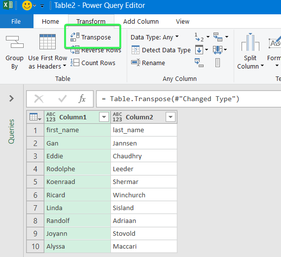
Meanwhile, you can use Power Query to transpose rows to columns. To do this, go to the Data tab, and create a query from table.

- Then select a range of cells to convert rows to columns in Excel. Click OK to open the Power Query Editor.

- In the Power Query Editor, go to the Transform tab and click Transpose. The rows will be rotated to columns.
- If you want to keep the headers for your columns, click the Use First Row as Headers button.
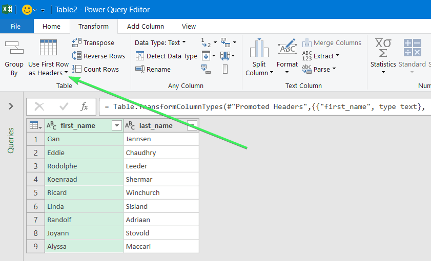
- That’s it. You can Close & Load your dataset – the rows will be converted to columns.

Error message when trying to convert rows to columns in Excel
To wrap up with converting Excel data in columns to rows, let’s review the typical error messages you can face during the flow.
Overlap error

The overlap error occurs when you’re trying to paste the transposed range into the area of the copied range. Please avoid doing this.
Wrong data type error

You may see this #VALUE! error when you implement the TRANSPOSE formula in Excel desktop without pressing Ctrl+Shift+Enter.
Other errors may be caused by typos or other misprints in the formulas you use to convert groups of data from rows to columns in Excel. Always double-check the syntax before pressing Enter or Ctrl+Shift+Enter 🙂 . Good luck with your data!
-

A content manager at Coupler.io whose key responsibility is to ensure that the readers love our content on the blog. With 5 years of experience as a wordsmith in SaaS, I know how to make texts resonate with readers’ queries✍🏼

Back to Blog
Focus on your business
goals while we take care of your data!
Try Coupler.io
Watch Video – The best way to Move Rows / Columns in Excel
Sometimes when working with data in Excel, you may have a need to move rows and columns in the dataset.
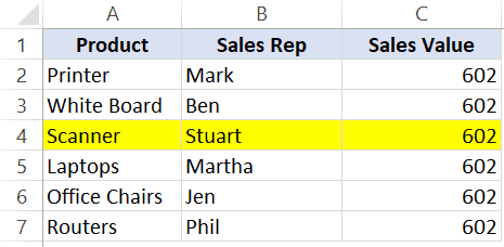
For example, in the below dataset, I want to quickly move the highlighted row to the top.
Now, are you thinking of copying this row, inserting the copied row where you want it, and then deleting it?
If yes – well that’s one way to do this.
But there is a lot faster way to move rows and columns in Excel.
In this tutorial, I will show you a fast way to move rows and columns in Excel – using an amazing shortcut.
Move Rows in Excel
Suppose I have the following dataset and I want to move the highlighted row to the second row (just below the headers):
Here are the steps to do this:
- Select the row that you want to move.
- Hold the Shift Key from your keyboard.
- Move your cursor to the edge of the selection. It would display the move icon (a four directional arrow icon).
- Click on the edge (with left mouse button) while still holding the shift key.
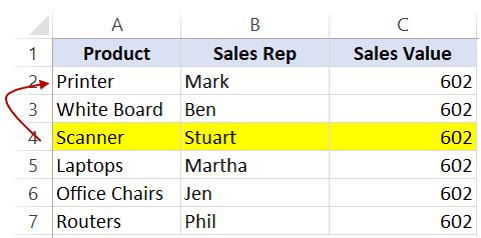
- Move it to the row where you want this row to be shifted
- Leave the mouse button when you see a bold line right below the row where you want to move this row.
- Leave the Shift-key (remember to keep the Shift key pressed till the end)
Below is a video that shows how to move a row using this method.
Note that in this example, I have moved the selected cells only.
If you want to move the entire row, you can select the entire row and then follow the same steps.
Here are some important things to know about this method:
- You can move contiguous rows (or some cells from the contiguous rows). You can’t move non-contiguous rows using this method. For example, you can’t move row # 4 and 6 at the same time. However, you can move row #5 and 6 at the same time by selecting it.
- When you move some cells in a row/column using this method, it will not impact any other data in the worksheet. In the above example, any data outside (above/below or to the right/left of this table) remains unaffected.
Move Columns in Excel
The same technique can also be used to move columns in Excel.
Here are the steps:
- Select the column (or contiguous columns) that you want to move.
- Hold the Shift Key from your keyboard.
- Move your cursor to the edge of the selection. It would display the move icon (a four directional arrow icon).
- Click on the edge (with left mouse button) while still holding the shift key.
- Move it to the column where you want this row to be shifted
- Leave the mouse button when you see a bold line to the edge of the column where you want to move this column.
- Leave the Shift-key (remember to keep the Shift key pressed till the end).
You May Also Like the Following Excel Tutorials:
- Quickly select blank cells in Excel.
- Quickly select a far-off cell/range in Excel.
- Keyboard and Mouse tricks that will reinvent the way you Excel.
- Highlight every other row in Excel.
- Insert New Cells in Excel.
- Highlight Active Row/Column in a dataset.
- Delete rows based on cell value in Excel
- Insert New Columns in Excel
(Note: This guide on how to change row height in Excel is suitable for all Excel versions including Office 365)
Excel consists of a multitude of cells. These cells are arranged in rows and columns for easy data entry and retrieval.
By default, the rows and columns appear with a specific height and width. Sometimes, when you enter data in the cells, the rows and columns might adjust to the height and width of the content. In most cases, the content will be hidden unless you enter the edit mode or double-click on the cell. In some cases, this can even cause a # error.
When the data in multiple cells exceed the display width, it’ll be hard to view the data. This hinders the readability of the data and makes the data look incomplete.
In such cases, you can change the row height or the column width to make the data in the cell easily readable to the user.
In this article, I will tell you how to change row height in Excel.
You’ll Learn:
- How to Change Row Height in Excel?
- By Clicking and Dragging
- By Double Clicking
- By Using AutoFit Rows
- By Changing the Row Height Manually
- Using Excel Hotkeys
Watch this short video on How to Change Row Height in Excel
Related Reads:
How to Make Excel Track Changes in a Workbook? 4 Easy Tips
How to Split Cells Diagonally in Excel? 2 Easy Ways
How to Merge Cells in Excel? 3 Easy Ways
How to Change Row Height in Excel?
There are a variety of ways to change row height in Excel. Some methods are used to change the row height for particular cells, whereas others help to change the row height or column width to suit the data in the cells.
Let us see each method in detail with an example.
Consider an Excel workbook that has the following data.

At first glance, it seems as though the data perfectly fit in each cell. Upon taking a closer look, it can be seen that the data visible to the user is not the actual data. Some of the text is hidden within the cells, which makes it difficult for the reader to understand and infer the contents of the cell.
In these cases, changing the row height and column width will enable you to understand the complete data. Let us see each method in detail.
By Clicking and Dragging
This is a prevalent and frequently used way to change row height or column width in Excel. By clicking and dragging, you can change the height and width of cells in Excel.
- First, identify the cell that you want to change the height or width of.
- If you want to change the row height, place your cursor on the row headings on the left side of the sheet. And, in case you want to change the column width, move the cursor to the column headings on the top of the sheet.

- Once you hover over the row or column headers, you can see the mouse pointer change to a double-sided resize pointer.
- Now by holding the left mouse button, drag to the desired height/width.
- Leave the mouse button.
- This sets the height of the particular row.
In the same way, you can set the column width to get a perfect readable view.

This method is a simple and easy method to change the row height. However, one drawback to this method is that when data is large, you have to click and drag every row. Also, when you change the height of one particular row, the other row’s height might get altered.
Let us now see the other methods to change the row height in Excel.
By Double Clicking
This is a very fast and easy method to change row height in Excel. Instead of altering the row height or column width, this method sets the height or width to perfectly fit the content in the cell.
- Place the mouse pointer in between the rows where you want to change the height.
- You can see the mouse pointer change to a double-sided resize pointer.
- Double click on the place and you can see the row height change to fit the content in the cell. You can see that if the row or column is expanded, double-clicking on the row shortens it. On the other hand, if the row is shortened, double-clicking expands it.
Note: To adjust the row height for multiple cells together, select all the cells and double-click on the row header.
By Using AutoFit Rows
In most cases when changing the row height, you would aim to make the contents of the cell visible. Double-clicking on the rows/column fits the rows and columns to the perfect height. Let us see how.
- Select the cells you want to adjust the height.
- Navigate to Home. Under the Cells section, click on the dropdown from Format.
- Since we want to adjust the row height, click on AutoFit Row Height.

- This instantly adjusts the row height to fit the content of the cells. This way, you can adjust the row height for any number of cells altogether.

Suggested Reads:
How to Unmerge Cells in Excel? 3 Best Methods
How to Enable Full Screen in Excel? 3 Simple Ways
How to Insert a Hyperlink in Excel? 3 Easy Ways
By Changing the Row Height Manually
When you change the row height by clicking and dragging or by double-clicking, you will not know the height or width value you set the rows or columns to. There might be times when you have to set the row height or column width to a specific value.
- First, select the rows that you want to change the height. To do this, navigate to the row header where you can see the mouse pointer change to an arrow.
- Left-click and hold the mouse button to select the rows.
- Now, right-click on the row headings and select Row Height.

- Another way to select Row Height is by navigating to Home. Under the Cells section, click on the dropdown from Format and select Row Height.
- This opens the Row Height dialog box.
- Specify the row height you want and click OK.

- This sets the row height to the specific units you have entered.
- If you are not satisfied with the row height, you can select the rows, change the value again, and click OK.

One advantage is that when you use this method and set the row height, all the rows will have the same height. This helps the rows and columns look aesthetically similar as they all have uniform spacing.
Using Excel Hotkeys
Keyboard shortcuts always help in quick and efficient ways to solve problems. Using keyboard shortcut keys also known as hotkeys, you can change the row height in Excel.
- Open the worksheet.
- Select the rows you want to change height either by clicking on the left mouse button and dragging them. Or hold shift and use the arrow keys to select the rows.
- Press the ALT key. This opens the hotkeys layout in the Excel window.
- Now press H and then O. This opens the Format dropdown.
- You can see the keyboard shortcut keys which correspond to specific options in the Format dropdown. If you want to set the row height to a specific value, press H. In case you want to autofit the row height to the content in the cells, press A.

Note: In the same way, you can change the column width easily using the shortcut keys. Press the keys Alt + H + O + W one after the other to change the column width.
Also Read:
How to Save Excel Chart as Image? 4 Simple Ways
How to Create Excel Drop Down List With Color?
How to Save Excel as PDF? 5 Useful Ways
Frequently Asked Questions
Why cannot I alter the row height in Excel?
You cannot alter the row height or column width when entering the edit mode in any cell. To exit the edit mode, click anywhere outside the particular cell or click on the row or column headings. When you see a single selection arrow or a double-sided resize arrow, you can change row height in Excel.
What is the easy and efficient way to change row height in Excel so that all content is visible?
The easiest and most efficient way to change the row height to fit the content is by selecting all the rows you want to change the height and double-clicking on the row. This changes the row height to fit the contents of the cell in an instant.
Can I change row height in Excel just by using keyboard shortcuts?
Yes, you can change the row height using the keyboard shortcut keys. Select the rows by holding the Shift key and using the arrow keys to select the cells. Then, press the shortcut keys Alt+H+O+H to set the row height manually. If you want to autofit the row height, press the keys Alt+H+O+A.
Closing Thoughts
Changing the row height or column width is a very essential feature. This helps simplify large amounts of data that may be hidden or intertwined in the cells, confusing the users. Simplified data, on the other hand, is easy for the user to read, understand, and perform operations to.
In this article, we saw how to change row height in Excel in 5 easy ways. Using the same methods, you can also change the column width. Depending on your preference and purpose, choose the method that suits you the best.
If you need more high-quality Excel guides, please check out our free Excel resources center. Simon Sez IT has been teaching Excel for over ten years. For a low, monthly fee you can get access to 140+ IT training courses. Click here for advanced Excel courses with in-depth training modules.

Simon Calder

Chris “Simon” Calder was working as a Project Manager in IT for one of Los Angeles’ most prestigious cultural institutions, LACMA.He taught himself to use Microsoft Project from a giant textbook and hated every moment of it. Online learning was in its infancy then, but he spotted an opportunity and made an online MS Project course — the rest, as they say, is history!
While working on excel many times you would want to flip table rows and columns. In that case, excel provides two methods. First is the TRANSPOSE function and the second is paste special technique. Both have their benefits. Let us see by an example, how to convert rows to columns and columns to rows in excel using both methods.
Example: Switch Excel Rows to Columns
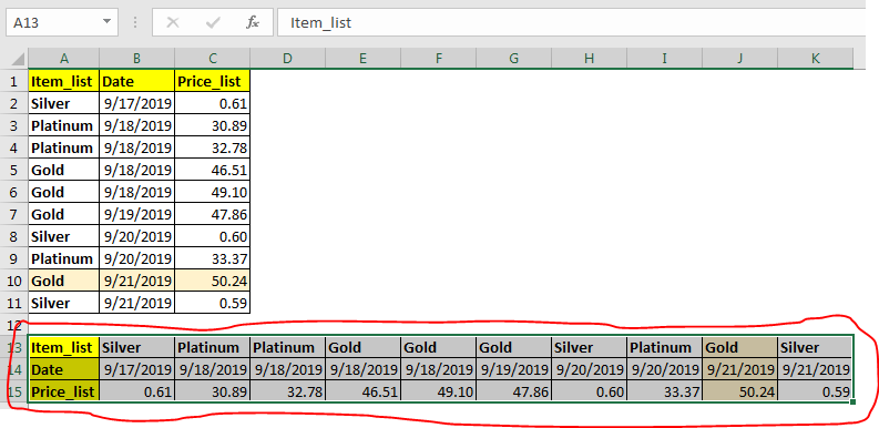
Here I have this table of price list of some items on different dates. Currently, the data is maintained column-wise. I want to switch rows to columns.
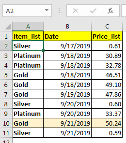
Convert rows to columns in excel using paste special
First, select the entire data including headings and footers. Copy it using CTRL+C shortcut. Now right-click on the cell where you want to transpose the table. Click on paste special. You can also use CTRL+ALT+V to open paste special dialogue.
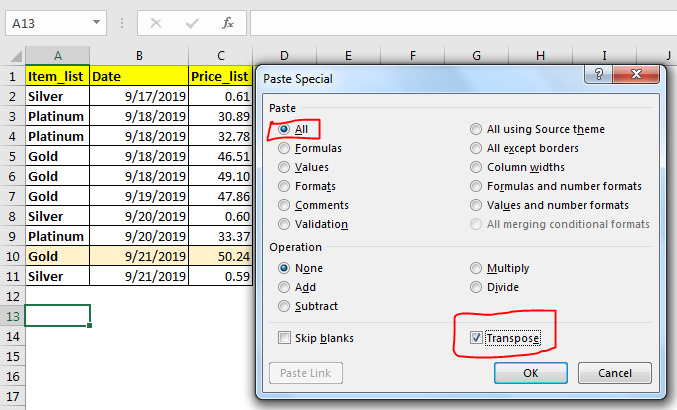
At the bottom-right, check the transpose checkbox. Hit the OK button.
The table is transposed. Rows are switched with columns.
Note: Use this when you want it to be done just once. It is static. For dynamic switching of columns with rows use excel TRANSPOSE function. It brings us to the next method.
Convert rows to columns in excel using the TRANSPOSE function
If you want dynamic switching of rows and columns in excel with an existing table. Then use the excel TRANSPOSE function.
The TRANSPOSE function is a multi-cell array formula. It means you have to predetermine how many rows and columns you’re gonna need and select that much area on sheet.
In the above example, we have 11×3 table in range A1:C11. To transpose we need to select 3×11 table. I selected A3:K15.
Since you selected the range, start writing this formula:
Hit CTRL+SHIFT+ENTER to enter as multi-cell array formula. You have your table switched. Rows data is now in columns and vice versa.

Note: This transposed table is linked with the original table. Whenever you change data in the original data, it will be reflected in the transposed table too.
Precaution: Before turning rows into columns make sure that you don’t have merged cells. With merged cell output may not be correct or may produce an error.
So yeah, this how you can switch table rows with columns. This is easy. Let me know if you have any doubts about this or any other query in excel 2016.
Popular Articles
50 Excel Shortcut to Increase Your Productivity: Get faster at your task. These 50 shortcuts will make you work even faster on Excel.
How to use the VLOOKUP Function in Excel: This is one of the most used and popular functions of excel that is used to lookup value from different ranges and sheets.
How to use the COUNTIF function in Excel: Count values with conditions using this amazing function. You don’t need to filter your data to count specific values. Countif function is essential to prepare your dashboard.
How to use the SUMIF Function in Excel: This is another dashboard essential function. This helps you sum up values on specific conditions.