
Reversing a string may not have many real-world applications, especially when working with spreadsheets. That is why you will not find any built-in function for this in Excel.
But there might be cases where you need to reverse a string, for whatever reason. Maybe you need to generate a special code, maybe you need to see if a string is a palindrome, or maybe you just want to do it for fun.
Even though there aren’t any built-in Excel functions for string reversal, there are a number of different ways to do this. You can use either a formula or a script written in VBA.
In this tutorial, we will see two ways to reverse a text string using a formula. If you like to use macros, then we also have a VBA script to help you reverse multiple strings quickly.
Reversing Text String using Text Formulas
Let us first understand the main process involved in reversing a string.
Let’s say you have a single cell with text that you want to reverse.
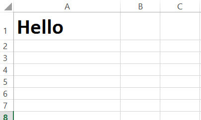
To reverse the string “Hello” in cell A1, follow these steps:
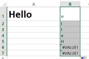
- In cell B1, type the following formula: =MID($A$1,LEN($A$1)-ROW(B1)+1,1). This should return the last character in the given string, which is “o”.
- Drag the fill handle down (situated at the bottom right of cell B1) until you start seeing “#VALUE!”.

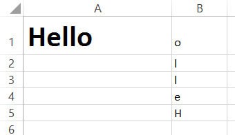
- You should now see each character of the string in “Hello” in each cell of column B, but reversed. Clear any cells containing “#VALUE!”. Here’s what you should finally see in our example:

- After the last cell of column B, i.e. in cell B6, type the formula: =TRANSPOSE(
- Drag and select the cells B1 to B5.
- Close the parentheses for the TRANSPOSE formula.
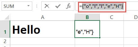
- Now select the whole formula in the formula bar and press F9 on your keyboard. This should display the values of each cell from B1 to B5, separated by commas and the whole thing should be surrounded by curly brackets: {“o”,”l”,”l”,”e”,”H”}.
- Remove the opening and closing curly brackets.
- Type “CONCATENATE”, followed by opening parentheses after the equal to sign.
- Close the parentheses after “H”.
- Press the return key.
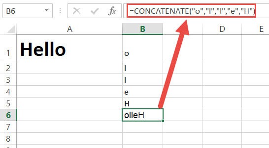
You should now see the reverse of the string “Hello” in cell B6.
What happened here?
Now let us look at what the formula did.
=MID($A$1,LEN($A$1)-ROW(B1)+1,1)
The function LEN($A$1) returns the length of the string in cell A1. We don’t want this cell reference to change when copied to the cells below B1, so we locked the cell reference by adding ‘$’ signs to it. The length of the string “Hello” is 5, so this function will return the value, ‘5’.
The function ROW(B1) simply returns the row number of cell B1. We might as well have typed ‘1’ instead of ‘ROW(B1)’, but wanted this value to change each time it was copied to a new cell. So when it’s copied to cell B2, it changes to value ‘2’. When copied to cell B3, it changed to value ‘3’ and so on.
Now, LEN($A$1)-ROW(B1)+1 gives us the value ‘5’, which is the index of the last character in “Hello”.
The function MID() returns the characters at a given index. It takes three parameters – A string or reference to a string, an index, and the number of characters to return starting at that index.
Here, the formula =MID($A$1,LEN($A$1)-ROW(B1)+1,1) takes the reference to cell A1 as the first parameter, the index, 5 as the second parameter and the number 1, as the third parameter. So the formula returns the character at index 5 of cell A1. This means we get the value “o” – the last character of the string.
Here’s what’s happening when you break down the formula:
- =MID($A$1,LEN($A$1)-ROW(B1)+1,1)
- =MID($A$1, 5 – 1 + 1, 1)
- =MID($A$1, 5, 1)
- =”o”
What happens when the formula is copied to cell B2?
In cell B2, the formula now changes to:
=MID($A$1,LEN($A$1)-ROW(B2)+1,1)
Here’s what’s happening when you break down the formula:
- =MID($A$1,LEN($A$1)-ROW(B2)+1,1)
- =MID($A$1, 5 – 2 + 1, 1)
- =MID($A$1, 4, 1)
- =”l”
What happens when the formula is copied to cell B5?
In cell B5, the formula now changes to:
=MID($A$1,LEN($A$1)-ROW(B5)+1,1)
Here’s what’s happening when you break down the formula:
- =MID($A$1,LEN($A$1)-ROW(B5)+1,1)
- =MID($A$1, 5 – 5 + 1, 1)
- =MID($A$1, 1, 1)
- =”H”
So the function returns the first character of the string in A1.
Although the above method works fine, it is not very practical as you would need to involve a whole lot of cells in your sheet. We demonstrated the above method just to break down the technique and make it easy for you to understand what’s happening.
Here’s a shortened down and more practical version of the above technique:
- In cell B1, type the formula:
=TRANSPOSE(MID(A1,LEN(A1)-ROW(INDIRECT("1:"&LEN(A1)))+1,1)) in cell B1. - Select the entire formula in the formula bar and press F9 on your keyboard.
- This should display each character of your string, reversed and separated by commas. The whole thing should be also surrounded by curly brackets, which means this is an array: {“o”,”l”,”l”,”e”,”H”}.

- Remove the opening and closing curly brackets.
- Type “CONCATENATE”, followed by opening parentheses after the equal to sign.
- Close the parentheses after “H”.
- Press the return key.

You should now see the reverse of the string “Hello” in cell B1. This calculation got done directly and in one cell. So it is a much more efficient way of using the formula to reverse a string.
There are a few things to note about this technique though:
- The reversed string will not change when you change the value in cell A1. You will need to repeat this process every time there’s a change.
- This method is alright if you have a few strings that you want to reverse, but if you have a whole list of strings to reverse, it might prove to be a little painstaking. This is because you need to always repeat steps 2 to 7 for every string.
Due to the above 2 disadvantages, we recommend using a VBA script to reverse text string in Excel.
Reversing Characters of a Text String in Excel using VBA Macro
Using VBA might sound a little intimidating if you’ve never used it before, but it can be an easier method to reverse strings in your worksheet.
Here’s the VBA code that we will be used to reverse a string in a single cell. Feel free to select and copy it.
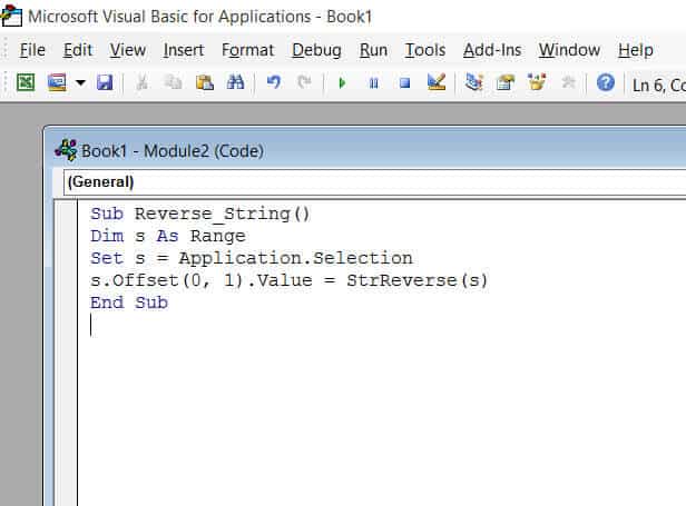
Sub Reverse_String()
Dim s As Range
Set s = Application.Selection
s.Offset(0, 1).Value = StrReverse(s)
End Sub
Follow these steps:
- From the Developer Menu Ribbon, select Visual Basic.
- Once your VBA window opens, Click Insert->Module. Now you can start coding. Type or copy-paste the above lines of code into the module window. Your code is now ready to run.

- Select a single cell containing the text you want to reverse. Make sure the cell horizontally next to it is blank because this is where the macro will display the reversed string.
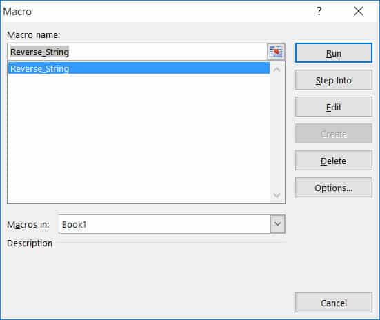
- Navigate to Developer->Macros->Reverse_String->Run.

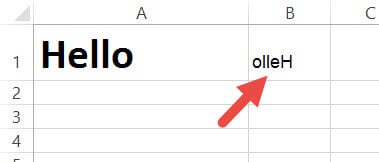
You will now see the reversed string next to your selected cell.
Note: If you can’t see the Developer ribbon, from the File menu, go to Options. Select Customize Ribbon and check the Developer option from the Main Tabs.
Finally, Click OK.
Reversing a List of Strings in Excel using VBScript
Using VBScript to reverse a long list of strings is easy too! Say you want to reverse the following set of names:
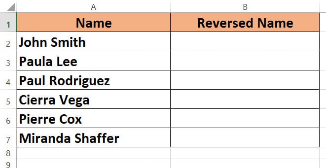
Here’s the VBA code that we will be using to reverse all strings in a column. Select and copy it.
Sub reverse_string_range()
Dim s As Range
Dim cell As Range
Set s = Application.Selection
i = 0
For Each cell In s
cell.Offset(0, 1).Value = StrReverse(cell)
i = i + 1
Next cell
End Sub
Follow these steps:
- From the Developer Menu Ribbon, select Visual Basic.
- Once your VBA window opens, Click Insert->Module. Now you can start coding. Type or copy-paste the above lines of code into the module window. Your code is now ready to run.
- Select the range of cells containing the text you want to reverse. Make sure the column next to it is blank because this is where the macro will display the reversed strings.
- Navigate to Developer->Macros->reverse_string_range->Run.
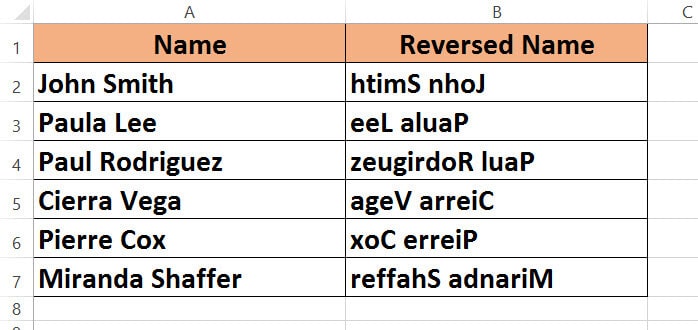
You will now see the reversed strings next to your selected range of cells.
Do remember to keep a backup of your sheet, because the results of VBA code are usually irreversible.
To wrap it up, we saw two ways to reverse strings in Excel. One method uses a formula and the other method uses VBA code.
The first method is alright if you don’t really feel comfortable working with VBA code. But it is beneficial only if you have one or a few cells that you want to reverse.
If there are more cells that need to be reversed, it can prove to be time-consuming.
Instead, you can use the second method (using VBA code), because it saves time and with just a few clicks, you can get a whole list of strings reversed in one go.
Although there are no straight ways to reverse a text string in Excel, I hope the methods shown here will help you get it done easily.
I hope you found this tutorial useful.
Other Excel tutorials you may find useful:
- How to Merge First and Last Name in Excel
- How to Split One Column into Multiple Columns in Excel
- How to Remove Commas in Excel (from Numbers or Text String)
- How to Generate Random Numbers in Excel (Without Duplicates)
- How to Add Text to the Beginning or End of all Cells in Excel
- How to Extract Number from Text in Excel (Beginning, End, or Middle)
- How to Change Uppercase to Lowercase in Excel
- How to Find the Last Space in Text String in Excel?
- Switch First and Last Name with Comma in Excel (Flip Names)
This tutorial will demonstrate how to reverse text in a cell in Excel & Google Sheets.
Reverse Text – Simple Formula
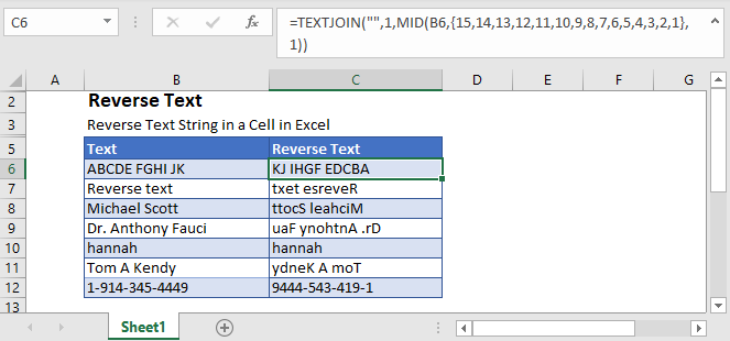
The simplest way to reverse a text string in Excel is with the TEXTJOIN and MID functions.
=TEXTJOIN("",1,MID(B6,{15,14,13,12,11,10,9,8,7,6,5,4,3,2,1},1))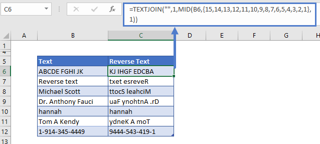
Note: This formula will only work for text with 15 characters or less. To work with longer text strings, you must add a larger array constant or use the Dynamic Array formula below.
How Does this Formula Work?
The MID Function extracts character(s) from a string of text. In our example, we told the MID Function to only extract one character. Then by defining the array constant {15,14,13,12,11,10,9,8,7,6,5,4,3,2,1} as the start position, the MID Function will output the text in reverse order.
The TEXTJOIN Function joins the array constant result together, outputting the text in reverse order.
Reverse Text – Dynamic Array
The simple formula will only reverse the first fifteen characters. To reverse more characters you would need to add to the array constant, or you can use the dynamic formula shown below.
The dynamic formula consists of the TEXTJOIN, MID, ROW, INDIRECT, and LEN functions.
Step 1
The first step is to calculate the total number of characters in the text string and generate an array of numbers corresponding to the number of characters:
=ROW(INDIRECT("1:"&LEN(B3)))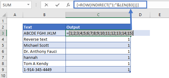
The above formula is an array formula and you can also convert the formula into array formula by pressing Ctrl + Shift + Enter. This is going to add curly brackets {} around the formula (note: this is not necessary in versions of Excel after Excel 2019).
Note: When these Formulas are entered in the cell, Excel will display only the first item in the array. To see the actual result of the array formula, you need to select the array formula cell and press F9 in the formula bar.
Step 2
Next reverse the array of numbers that were generated in the previous step:
=LEN(B3)-ROW(INDIRECT("1:"&LEN(B3)))+1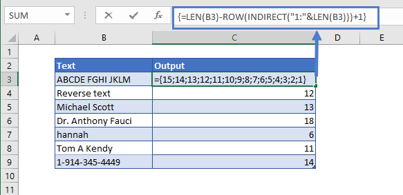
Step 3
Now use the MID Function to extract the text.
This formula will reverse the order of the array during extraction by taking the characters from right to left.
=MID(B3,LEN(B3)-ROW(INDIRECT("1:"&LEN(B3)))+1,1)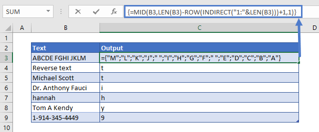
Final Step
Last use the TEXTJOIN Function to join together the individual characters.
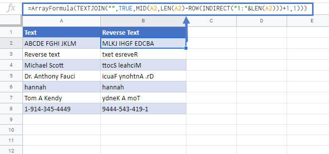
=TEXTJOIN("",TRUE,MID(B3,LEN(B3)-ROW(INDIRECT("1:"&LEN(B3)))+1,1))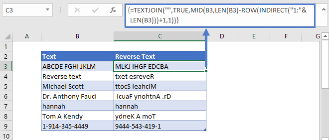
Reverse Text In Google Sheets
The formula to reverse text works exactly the same in Google Sheets as in Excel. Except when you close the formula with CTRL + SHIFT + ENTER, Google Sheets adds the ARRAYFORMULA function around the formula.
Хитрости »
4 Май 2011 57885 просмотров
Как перевернуть слово?
Не самая распространенная, но тем не менее встречающаяса задача: перевернуть слово. Т.е. расположить буквы слова в обратном порядке. Из «привет» сделать «тевирп». Если честно, то сейчас затрудняюсь озвучить конкретную ситуацию, в которой это может пригодиться. Сам использовал когда-то в случае, когда надо было перевернуть числовые значения с еще некоторыми манипуляциями. Но ситуации бывают разные, как и решения задачи, которых несколько.
Сначала я хотел бы описать способы переворачивания слова средствами VBA, т.к. именно они кажутся мне наиболее рациональными и наиболее удобными для большинства, несмотря на необходимость использовать VBA.
Способ 1:
Через встроенную функцию VBA StrReverse(). Быстрый и короткий. Самый удобный. Но работает только начиная от Excel 2000 и выше.
Sub Reverse_Word()
    On Error Resume Next
    ActiveCell.Value = StrReverse(ActiveCell.Value)
End Sub
Чтобы применить этот код необходимо слегка погрузиться в мир Visual Basic for Applications: переходим в редактор VBA(Alt+F11) —Insert —Module. Вставляем туда приведенный выше код. Выделяем ячейку с любым словом -Alt+F8 -Reverse_Word -Выполнить. Слово в активной ячейке будет перевернуто.
Способ 2:
Более медленный, содержит больше строк кода, но работает во всех версиях:
Sub Reverse_Word()
    Dim sWord As String, sReverseWord As String
    Dim li As Long
    sWord = ActiveCell.Value
    For li = Len(sWord) To 1 Step -1
        sReverseWord = sReverseWord & Mid(sWord, li, 1)
    Next li
    ActiveCell.Value = sReverseWord
End Sub
Код применяется точно так же, как и первый.
Оба эти кода можно сделать функциями пользователя, чтобы вызывать их с листа Excel как любую другую функцию:
' Функция работает с версиями Excel, начиная с 2000
Function Reverse_Word(sWord As String)
    Reverse_Word = StrReverse(sWord)
End Function

' Функция работает со всеми версиями Excel
Function Reverse_Word_All(sWord As String)
    Dim sReverseWord As String
    Dim li As Long
    For li = Len(sWord) To 1 Step -1
        sReverseWord = sReverseWord & Mid(sWord, li, 1)
    Next li
    Reverse_Word_All = sReverseWord
End Function
Чтобы правильно использовать приведенные выше коды, необходимо сначала ознакомиться со статьей Что такое функция пользователя(UDF)?. Вкратце: необходимо скопировать текст кода выше, перейти в редактор VBA(Alt+F11) -создать стандартный модуль(Insert —Module) и в него вставить скопированный текст. После чего функцию можно будет вызвать из Диспетчера функций, отыскав её в категории Определенные пользователем (User Defined Functions).
Способ 3: стандартными функциями в любой версии Excel
Сразу хочу оговориться — стандартными формулами сделать это хоть и можно, но не совсем просто и совершенно неудобно. Для этого потребуется гораздо больше манипуляций, чем через VBA. Хотя для кого-то, возможно, способ формулами будет более прост, чем через VBA. Для начала необходимо будет включить итеративные вычисления в функциях:
- Excel 2003: Сервис -Параметры -Вычисления -ставим галочку Итерации
- Excel 2007: Меню -Параметры Excel -Формулы -Включить итеративные вычисления
- Excel 2010 и выше: Файл -Параметры -Формулы -Включить итеративные вычисления
Устанавливаем предельное число итераций — 1. Если слово, которое необходимо перевернуть записано в ячейке А1, то формула будет выглядеть следующим образом:
=ЕСЛИ(ДЛСТР(B1)>=ДЛСТР(A1);B1;ЕСЛИ(ДЛСТР(B1)=1;ПСТР(A1;ДЛСТР(A1);1);B1)&ПСТР(A1;ДЛСТР(A1)-ДЛСТР(B1);1))
=IF(LEN(B1)>=LEN(A1),B1,IF(LEN(B1)=1,MID(A1,LEN(A1),1),B1)&MID(A1,LEN(A1)-LEN(B1),1))
Но в данном случае мало просто записать формулу. При внесении формулы в ячейку она сразу не выдаст необходимый результат. Необходимо пересчитывать формулу до тех пор, пока все слово не перевернется(я просто нажал и удерживал клавишу F9). Эту формулу я придумал чисто «из спортивного интереса». Но кому-то, возможно, будет гораздо проще так, чем через VBA.
В приложенном к статье файле помимо рассмотренных примеров есть еще один вариант решения формулами, который лично мне не нравится своей очевидностью, а главное — он «растягивается» на несколько ячеек. Это не очень удобно, но избавляет от необходимости включать итерации. Хотя на мой взгляд это единственный положительный момент в данном способе:
=ЕСЛИ(СТОЛБЕЦ(A1)>ДЛСТР($A2);»»;B2&ПСТР($A2;ДЛСТР($A2)+1-СТОЛБЕЦ(A1);1))
=IF(COLUMN(A1)>LEN($A2),»»,B2&MID($A2,LEN($A2)+1-COLUMN(A1),1))
Слово в ячейке $A2, B2 должна быть пустой, а уже с C2 начинается формула.
При желании можно в какой-либо другой ячейке записать формулу сцепления всех полученных ячеек с запасом, чтобы получить единое слово в обратном порядке.
Функция для Excel 2016 и выше
А для счастливых обладателей Excel 2016, 365 и выше можно использовать простую и гибкую формулу массива(вводится в ячейки такая формула сочетанием трех клавиш Ctrl+Shift+Enter):
=ОБЪЕДИНИТЬ(«»;0;ЕСЛИОШИБКА(ПСТР(A1;ДЛСТР(A1)-СТРОКА(A1:A999)+1;1);»»))
=TEXTJOIN(«»,0,IFERROR(MID(A1,LEN(A1)-ROW(A1:A50000)+1,1),»»))
Если текст слишком длинный необходимо лишь расширить диапазон A1:A999 с чуть большим запасом, например: A1:A50000. 50 000 букв точно хватит 
Никаких макросов и итераций — все же Microsoft думает о нас, о пользователях и внедряет всякие новые плюшки.
Скачать пример
 Tips_All_ReverseWord.xls (74,5 KiB, 3 772 скачиваний)
Так же см.:
Функция перемещения слова в строке
Надстройка для замены и перемещения слов/аббревиатур
Как перевернуть адрес
Статья помогла? Поделись ссылкой с друзьями!
![]() Видеоуроки
Видеоуроки
Поиск по меткам
Access
apple watch
Multex
Power Query и Power BI
VBA управление кодами
Бесплатные надстройки
Дата и время
Записки
ИП
Надстройки
Печать
Политика Конфиденциальности
Почта
Программы
Работа с приложениями
Разработка приложений
Росстат
Тренинги и вебинары
Финансовые
Форматирование
Функции Excel
акции MulTEx
ссылки
статистика
When you use the Excel worksheet, how do you reverse the text string or words order in Excel? For example, you want to reverse “Excel is a useful tool for us” to “su rof loot lufesu a si lecxE”. Or sometimes you may reverse the words order such as “Excel, Word, PowerPoint, OneNote” to “OneNote, PowerPoint, Word, Excel”. Normally this is somewhat difficult to solve this problem. Please look at the following methods:
Reverse text string with User Defined Function
Reverse words order separated by specific separator with VBA code
Reverse text string or words order with Kutools for Excel quickly and easily
 Reverse text string with User Defined Function
Supposing you have a range of text strings which you want to reverse, such as “add leading zeros in Excel” to “lecxE ni sorez gnidael dda”. You can reverse the text with following steps:
1. Hold down the ALT + F11 keys, and it opens the Microsoft Visual Basic for Applications window.
2. Click Insert > Module, and paste the following macro in the Modulewindow.
Function Reversestr(str As String) As String
    Reversestr = StrReverse(Trim(str))
End Function
3. And then save and close this code, go back to the worksheet, and enter this formula: =reversestr(A2) into a blank cell to put the result, see screenshot:

4. Then drag the fill handle down to copy this formula, and the text in the cells is revered at once, see screenshot:

Reverse words order separated by specific separator with VBA code
If you have a list of cell words which are separated by commas as this “teacher, doctor, student, worker, driver”, and you want to reverse the words order like this “drive, worker, student, doctor, teacher”. You can also use follow VBA to solve it.
1. Hold down the ALT + F11 keys, and it opens the Microsoft Visual Basic for Applications window.
2. Click Insert > Module, and paste the following macro in the Module window.
Sub ReverseWord()
'Updateby Extendoffice
Dim Rng As Range
Dim WorkRng As Range
Dim Sigh As String
On Error Resume Next
xTitleId = "KutoolsforExcel"
Set WorkRng = Application.Selection
Set WorkRng = Application.InputBox("Range", xTitleId, WorkRng.Address, Type:=8)
Sigh = Application.InputBox("Symbol interval", xTitleId, ",", Type:=2)
For Each Rng In WorkRng
    strList = VBA.Split(Rng.Value, Sigh)
    xOut = ""
    For i = UBound(strList) To 0 Step -1
        xOut = xOut & strList(i) & Sigh
    Next
    Rng.Value = xOut
Next
End Sub3. Then press F5 key, a dialog is displayed, please select a range to work with. See screenshot:

4. And then press Ok, another dialog is popped out for you to specify the separator that you want to reverse the words based on, see screenshot:

5. Then click OK, and you can see the words selected are reversed, see screenshots:
Reverse text string or words order with Kutools for Excel quickly and easily
The Kutools for Excel’s Reverse Text Order can help you quickly and conveniently to reverse various text strings. It can do following operations:
Reverse the text from right to left, such as “tap some words” to “sdrow emos pat”;
Reverse the text are separated by space or other specific characters, such as “apple orange grape” to “grape orange apple”;
Reverse the text from right to left:
1. Select the range that you want to reverse.
2. Click Kutools > Text Tools > Reverse Text Order, see screenshot:

3. In the Reverse Text dialog box, select the proper option from Separator which are corresponding with the cell values. And you can preview the results from the Preview Pane. See screenshot:

Download and free trial Kutools for Excel Now !
Reverse the text are separated by space or other specific characters:
This feature also can help you to reverse the text strings which are separated by specific characters.
1. Select the cells and apply this utility by clicking Kutools > Text > Reverse Text Order.
2. In the Reverse Text dialog box, choose the separator which separate the cell values that you want to reversed the words based on, see screenshot:

3. Then click Ok or Apply, the words in the cells have been reversed at once. See screenshots:
Note:Checking Skip non-text cells to prevent you reversing the numbers in selected range.
To know more about this function, please visit Reverse Text Order.
Download and free trial Kutools for Excel Now !
Demo: Reverse text string based on specific separator with Kutools for Excel
Kutools for Excel: with more than 300 handy Excel add-ins, free to try with no limitation in 30 days. Download and free trial Now!
Related article:
How to flip the first and last name in cells in Excel?
The Best Office Productivity Tools
Kutools for Excel Solves Most of Your Problems, and Increases Your Productivity by 80%
- Reuse: Quickly insert complex formulas, charts and anything that you have used before; Encrypt Cells with password; Create Mailing List and send emails…
- Super Formula Bar (easily edit multiple lines of text and formula); Reading Layout (easily read and edit large numbers of cells); Paste to Filtered Range…
- Merge Cells/Rows/Columns without losing Data; Split Cells Content; Combine Duplicate Rows/Columns… Prevent Duplicate Cells; Compare Ranges…
- Select Duplicate or Unique Rows; Select Blank Rows (all cells are empty); Super Find and Fuzzy Find in Many Workbooks; Random Select…
- Exact Copy Multiple Cells without changing formula reference; Auto Create References to Multiple Sheets; Insert Bullets, Check Boxes and more…
- Extract Text, Add Text, Remove by Position, Remove Space; Create and Print Paging Subtotals; Convert Between Cells Content and Comments…
- Super Filter (save and apply filter schemes to other sheets); Advanced Sort by month/week/day, frequency and more; Special Filter by bold, italic…
- Combine Workbooks and WorkSheets; Merge Tables based on key columns; Split Data into Multiple Sheets; Batch Convert xls, xlsx and PDF…
- More than 300 powerful features. Supports Office / Excel 2007-2021 and 365. Supports all languages. Easy deploying in your enterprise or organization. Full features 30-day free trial. 60-day money back guarantee.
")
Office Tab Brings Tabbed interface to Office, and Make Your Work Much Easier
- Enable tabbed editing and reading in Word, Excel, PowerPoint, Publisher, Access, Visio and Project.
- Open and create multiple documents in new tabs of the same window, rather than in new windows.
- Increases your productivity by 50%, and reduces hundreds of mouse clicks for you every day!
")
We can use a single formula (code) to reverse a text string (text reverser) in Excel 365. You heard me right!
It is possible because of the Spill feature and the availability of the functions SEQUENCE and TEXTJOIN in this iteration of Excel.
In the old school method, we usually use multiple formulas or a VBA for reversing a Text in Excel. Those days are gone if you are using Excel 365.
What do we expect the formula to do?
If cell A1 contains ABC, we require a single formula to return CBA in cell B1.
If it is ABC 123, we expect 321 CBA.
Here is our text reverser formula to use in Excel 365.
=TEXTJOIN("",TRUE,MID(A1,SEQUENCE(LEN(A1),1,LEN(A1),-1),1))
How does this formula work in Excel 365?
We have already learned how to split a string into a list of characters in Excel 365.
That formula will help us to extract each character from a cell into multiple cells.
We have used a similar approach here.
Since we want to reverse the text, here, on the contrary, we have extracted individual characters from the last part of the string.
Anatomy of the Text Reverser Formula
Let’s peel the above formula to learn how it works in Excel 365. For the test, we will use the flower name ROSE.
There are four characters in the above flower name.
Using the following MID, we can take out each character beginning from the end of the string ROSE.
=MID(A1,4,1)
=MID(A1,3,1)
=MID(A1,2,1)
=MID(A1,1,1)
Syntax: MID(text, start_num, num_char)
We may be able to convert it into a single piece of code in Excel 365 if we feed start_num with a reverse sequence formula that returns 4, 3, 2, 1.
The following Excel SEQUENCE formula will do that.
=SEQUENCE(4,1,4,-1)Syntax: SEQUENCE(rows, [columns], [start], [step])
So we can merge those four formulas into one as below.
=MID(A1,SEQUENCE(4,1,4,-1),1)The #4 in the above formula is the number of characters in the world ROSE.
Since we want to reverse any text, we should dynamically find the number of characters in the text.
We can do that using the Excel LEN function. I mean, we will replace 4 with the code LEN(A1).
Finally, the TEXTJOIN joins the reversed characters. That’s it.
Содержание
- Текст в ячейке задом наперёд
- Текст в ячейке задом наперёд
- Переворачиваем таблицы в обратную сторону средствами MS Excel
- Источник проблемы.
- Транспонирование.
- Используем для переворачивания функцию ИНДЕКС.
- Применяем функцию СМЕЩ.
- Действия после разворачивания таблицы и итоги работы.
- Переворачиваем с помощью сортировки
- Транспонирование (поворот) данных из строк в столбцы и наоборот
- Советы по транспонированию данных
- Дополнительные сведения
- Как перевернуть слово?
- Поиск по меткам
Текст в ячейке задом наперёд
Текст в ячейке задом наперёд
Добрый день, уважаемые читатели блога! Продолжаем серию уроков по Microsoft Excel и сегодня мы отойдём от привычного создания макросов, рассмотрения приёмов, различных тонкостей.
Поговорим о пользовательских функциях, то есть о функциях, которые может создавать сам пользователь, оперируя переменными Excel.
Перед нами стоит задача — отобразить текст в ячейке (произвольный) в обратном порядке. Пример: «Привет!», — в соседней ячейке появится: «!тевирП».
В таком случае можно использовать макрос, но количество действий, его (макроса) постоянный вызов не улучшат, а затруднят работу с таблицей.

Воспользуемся возможностью создания своих функций. Благо для этого нам подойдёт алгоритм создания макроса.
Добавляем новый модуль в наш документ:
- Вкладка «Разработчик», блок кнопок «Код», кнопка «Visual Basic»;
- Далее «Insert» — > «Module».

Добавим следующий текст в наш модуль:
Function dhReverseText(strText As String) As String
Dim i As Integer
For i = Len(strText) To 1 Step -1
dhReverseText = dhReverseText & Mid(strText, i, 1)
Next i
End Function

Разберём где у нас что:
- «Function dhReverseText(strText As String) As String» — название функции и объявление её типом строка;
- « Dim i As Integer» — объявление переменной i;
- «For i = Len(strText) To 1 Step -1» — для каждой переменной i типа строка устанавливаем обратный порядок расположения символов (Len — возвращает количество символов в ячейке);
- «dhReverseText = dhReverseText & Mid(strText, i, 1)» — указываем функции, что двигаться нужно от конца к началу;
- » Next i » — обработка следующего символа.
Прелестью такого подхода является работа с функцией, мы можем вводить её как простую формулу.
Источник
Переворачиваем таблицы в обратную сторону средствами MS Excel
Источник проблемы.
В ходе работы довольно часто встречаются ситуации, когда необходимо выполнить разворот таблиц определенным образом, в том числе разворот в обратном порядке столбцов.. Такой разворот таблиц может, к примеру, понадобиться, если требуется выполнить сортировку ячеек, расположенных по горизонтали.
Приведем пример. Мы имеем таблицу следующего вида:

Цена, а значит и сумма заказа по каждой позиции зависит от объема, то есть от количества заказанных единиц товара. В этом случае можно было бы применить функцию ГПР, но тогда цены должны быть указаны в порядке их повышения. Здесь же ситуация состоит с точностью до наоборот.
Транспонирование.
Наверное, это самый простой вариант решения проблемы. Необходимо скопировать нужную таблицу. После этого выбрать ячейку рядом и в специальной вставке выбрать вариант «транспонирование». В последних версиях Excel этот пункт вынесен в виде пиктограммы непосредственно в контекстное меню.

В результате мы переворачиваем таблицу на 90 градусов, и ее столбцы и строки поменяются местами. 
Как это использовать для переворачивания исходных столбцов? Очень просто! После транспонирования надо пронумеровать строчки с нужными данными. В нашем случае это выглядит так.

После этого выделяем нужные строки вместе с добавленной нами нумерацией, и запускаем с вкладки «Данные» настраиваемую сортировку.

В появившемся окне убираем, если стоит, галочку «мои данные содержат заголовки», в качестве первого уровня показываем столбец с нашей нумерацией и выбираем вариант сортировки по убыванию.

Осталось скопировать полученный результат, но без добавленного столбца с нумерацией и с помощью транспонирования вставить его на исходное место. После этого промежуточную таблицу можно удалить.
Теперь наша таблица уже выглядит следующим образом.

Остается заметить, что, если надо поменять в обратном порядке непосредственно строки, то выполнять транспонирование не требуется.
Преимуществом данного способа является прежде всего простота и доступность, а также отсутствие формул и функций. Однако метод имеет и недостатки. Прежде всего это трудоемкость. Кроме этого, имеется ограничение на количество столбцов. На листе Excel имеется только 16384 строки. Поэтому если у вас в таблице строк больше, а я сталкивался с таблицами и в 20000 строк, и в 200000 строк, и более чем в миллион строк, так вот в таком случае способ бесполезен и все-таки придется использовать формулы и функции
Используем для переворачивания функцию ИНДЕКС.
Наверное, это самый простой вариант для разворота таблицы в обратную сторону средствами MS Excel без предварительного транспонирования, который я смог найти на просторах интернета. Суть его состоит в том, что в качестве диапазона указываем строку, в которой надо поменять столбцы местами. Номер строки задаем равной 1, а в качестве номера столбца используем дополнительную функцию ЧИСЛСТОЛБ, в которой указываем заново этот же диапазон для разворачивания, но в адресе последней ячейки в ней закрепляем только столбец, используя смешанную адресацию

Данный способ, точнее данная составная функция, проще, чем следующие варианты из сети Интернет:
=ИНДЕКС (A$1:A$6;ЧСТРОК (A$1:A$6)+СТРОКА (A$1)-СТРОКА ()) =СМЕЩ ($A$6;(СТРОКА ()-СТРОКА ($A$1))*-1;0)
=ИНДЕКС ($A$1:$A$6;СЧЁТЗ ($A$1:$A$6)-СТРОКА ()+1)
=ИНДЕКС (A:A;СЧЁТЗ (A:A)-СТРОКА ()+1)
В отличии от всего этого мы использовали только две функции. Функция ИНДЕКС извлекает значение из диапазона на пересечении указанных по номеру в таблице строки и столбца. Строка была только одна, поэтому мы и написали единицу. Номер же столбца мы нашли с помощью функции ЧИСЛСТОЛБ. Вначале она показала номер последнего столбца, а затем из=-за примененной адресации этот номер стал уменьшаться и в итоге столбцы стали разворачиваться.
Учтите, что если надо было бы поменять местами строки, то надо уже указать диапазон из одного столбца. В формуле вместо единицы на месте номера строки надо было бы указать функцию ЧСТРОК и, выделив диапазон, в адресе последней ячейки уже закрепить только строку, оставив знак доллара только перед ее номером.
Применяем функцию СМЕЩ.
В данном случае необходимо добавить сверху таблицы новую строку и пронумеровать в ней нужные столбцы в обратном порядке, начиная с нуля. Удобно это сделать с помощью простой формулы, как на рисунке. Первый нуль мы указываем, конечно, сами с клавиатуры.

Формула же для разворачивания столбцов в обратном порядке будет уже выглядеть следующей. Мы будем использовать функцию СМЕЩ. В качестве исходного диапазона зададим последнюю ячейку в текущей обрабатываемой строке с закреплением только столбца, перемещение по строкам зададим равным 0, а смещение по столбцам сделаем равным первой ячейке в добавленной нами сверху строке, то есть нулю, и закрепим в адресе этой ячейке номер строки.
Результат перед вами. И обратите внимание на адресацию!

Действия после разворачивания таблицы и итоги работы.
Теперь, когда таблица развернута в противоположном по столбцам направлении, уже можно применить в частности функцию ГПР.
В данном случае она будет выглядеть так.

Более подробно о функциях ВПР и ГПР мы поговорим на следующих уроках.
Наше же текущее занятие подошло к концу. Желаю всем безошибочной работы и профессионализма на практике. Помните, что многие действия могут быть выполнены гораздо проще, чем кажется вначале. Не зря еще дедушка Крылов обронил в свое время фразу: «На мудреца довольно простоты … А ларчик просто открывался…
Всем успехов и уверенности в своих силах. Экспериментируйте, будьте аккуратными и внимательным и все будет получаться и становиться простым и легким!.
Переворачиваем с помощью сортировки
Для применения данного метода не требуется формул. Более того, сами перемещаемые пр развороте столбцы остаются в пределах своего диапазона, что так же является значитпельным плюсом. К тому же данный спгособ позволяет не только развернуть таблицу слева гнаправа, но и вывести колонки в любом порядке. Все очень просто. ПРедположим, нам надо развернуть стобцыв в таблице, рассмотренной выше. Для этого:
добавляем строку с нужным порядком столбцов. Ее можно добавить как выше заголовка таблицы, так и под ней. Выберем первый вариант.

Выделяем нужные столбцы вместе с добавленной номинацией и запускаем настраиваемую сортировку. В частности, это можно сделать с вкладки «Данные». Заходим в параметры и а выбираем вариант «Сортировать по столбцам диапазона»

Возвращаемся в настройку сортировки. В пункте «Сортировать по» указываем строку с заданным на первом этапе порядком столбцов и нажимаем ОК
Источник
Транспонирование (поворот) данных из строк в столбцы и наоборот
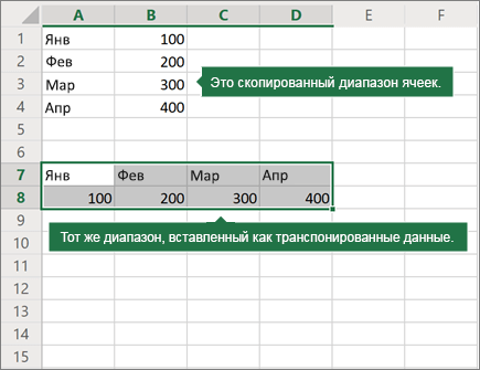
Если у вас есть таблица с данными в столбцах, которые необходимо повернуть для переупорядочивать их по строкам, используйте функцию Транспонировать. С его помощью можно быстро переключать данные из столбцов в строки и наоборот.
Например, если данные выглядят так: «Регионы продаж» в заголовках столбцов и «Кварталы» с левой стороны:
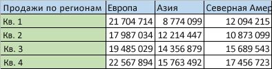
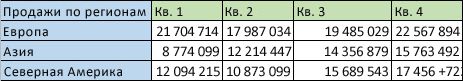
Функция Транспонировать переупомешет таблицу, в которой столбцы «Кварталы» отображаются в заголовках столбцов, а слева будут показаны регионы продаж, например:
Примечание: Если данные хранятся в таблице Excel, функция Транспонирование будет недоступна. Можно сначала преобразовать таблицу в диапазон или воспользоваться функцией ТРАНСП, чтобы повернуть строки и столбцы.
Вот как это сделать:
Выделите диапазон данных, который требуется переупорядочить, включая заголовки строк или столбцов, а затем нажмите клавиши CTRL+C.
Примечание: Убедитесь, что для этого нужно скопировать данные, так как не получится использовать команду Вырезать или CTRL+X.
Выберите новое место на том месте на компьютере, куда вы хотите ввести транспонную таблицу, чтобы вместить данные в достаточном месте. В новой таблице будут полностью переоформатироваться все данные и форматирование, которые уже есть.
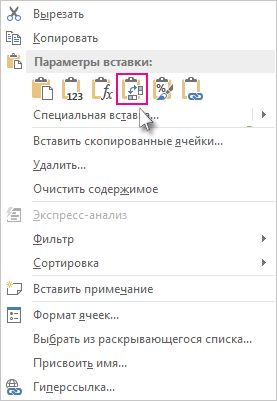
Щелкните правой кнопкой мыши левую верхнюю ячейку, в которой нужно ввести транспонировать таблицу, и выберите транспонировать  .
.
После успешного поворота данных можно удалить исходную таблицу, и данные в новой таблице останутся без изменений.
Советы по транспонированию данных
Если данные содержат формулы, Excel автоматически обновляет их в соответствие с новым расположением. Убедитесь, что в этих формулах используются абсолютные ссылки. Если они не используются, перед поворотом данных можно переключаться между относительными, абсолютными и смешанными ссылками.
Если вы хотите часто поворачивать данные для их просмотра под разными углами, создайте с помощью нее с помощью перетаскиванием полей из области строк в область столбцов (или наоборот)в списке полей.
Вы можете ввести в книгу данные в качестве транспон данных. Транспонировать: переупочевание содержимого скопированные ячейки при копировании. Данные строк будут вставлены в столбцы, и наоборот.
Вот как можно транспоннять содержимое ячейки:
Скопируйте диапазон ячеев.
Вы выберите пустые ячейки, в которые вы хотите ввести транспонировать данные.
На вкладке Главная щелкните значок Ввести и выберите Ввести транспонировать.
Дополнительные сведения
Вы всегда можете задать вопрос специалисту Excel Tech Community или попросить помощи в сообществе Answers community.
Источник
Как перевернуть слово?
Не самая распространенная, но тем не менее встречающаяса задача: перевернуть слово. Т.е. расположить буквы слова в обратном порядке. Из «привет» сделать «тевирп». Если честно, то сейчас затрудняюсь озвучить конкретную ситуацию, в которой это может пригодиться. Сам использовал когда-то в случае, когда надо было перевернуть числовые значения с еще некоторыми манипуляциями. Но ситуации бывают разные, как и решения задачи, которых несколько.
Сначала я хотел бы описать способы переворачивания слова средствами VBA, т.к. именно они кажутся мне наиболее рациональными и наиболее удобными для большинства, несмотря на необходимость использовать VBA.
Способ 1:
Через встроенную функцию VBA StrReverse(). Быстрый и короткий. Самый удобный. Но работает только начиная от Excel 2000 и выше.
Sub Reverse_Word() On Error Resume Next ActiveCell.Value = StrReverse(ActiveCell.Value) End Sub
Чтобы применить этот код необходимо слегка погрузиться в мир Visual Basic for Applications: переходим в редактор VBA( Alt+F11 ) —Insert —Module. Вставляем туда приведенный выше код. Выделяем ячейку с любым словом — Alt + F8 -Reverse_Word -Выполнить. Слово в активной ячейке будет перевернуто.
Способ 2:
Более медленный, содержит больше строк кода, но работает во всех версиях:
Sub Reverse_Word() Dim sWord As String, sReverseWord As String Dim li As Long sWord = ActiveCell.Value For li = Len(sWord) To 1 Step -1 sReverseWord = sReverseWord & Mid(sWord, li, 1) Next li ActiveCell.Value = sReverseWord End Sub
Код применяется точно так же, как и первый.
Оба эти кода можно сделать функциями пользователя, чтобы вызывать их с листа Excel как любую другую функцию:
‘ Функция работает с версиями Excel, начиная с 2000 Function Reverse_Word(sWord As String) Reverse_Word = StrReverse(sWord) End Function ‘ Функция работает со всеми версиями Excel Function Reverse_Word_All(sWord As String) Dim sReverseWord As String Dim li As Long For li = Len(sWord) To 1 Step -1 sReverseWord = sReverseWord & Mid(sWord, li, 1) Next li Reverse_Word_All = sReverseWord End Function
Чтобы правильно использовать приведенные выше коды, необходимо сначала ознакомиться со статьей Что такое функция пользователя(UDF)?. Вкратце: необходимо скопировать текст кода выше, перейти в редактор VBA( Alt+F11 ) -создать стандартный модуль(Insert —Module) и в него вставить скопированный текст. После чего функцию можно будет вызвать из Диспетчера функций, отыскав её в категории Определенные пользователем (User Defined Functions) .
Способ 3: стандартными функциями в любой версии Excel
Сразу хочу оговориться — стандартными формулами сделать это хоть и можно, но не совсем просто и совершенно неудобно. Для этого потребуется гораздо больше манипуляций, чем через VBA. Хотя для кого-то, возможно, способ формулами будет более прост, чем через VBA. Для начала необходимо будет включить итеративные вычисления в функциях:
- Excel 2003: Сервис -Параметры -Вычисления -ставим галочку Итерации
- Excel 2007: Меню -Параметры Excel -Формулы -Включить итеративные вычисления
- Excel 2010 и выше: Файл -Параметры -Формулы -Включить итеративные вычисления
Функция для Excel 2016 и выше
А для счастливых обладателей Excel 2016, 365 и выше можно использовать простую и гибкую формулу массива(вводится в ячейки такая формула сочетанием трех клавиш Ctrl + Shift + Enter ):
=ОБЪЕДИНИТЬ(«»;0;ЕСЛИОШИБКА(ПСТР( A1 ;ДЛСТР( A1 )-СТРОКА( A1:A999 )+1;1);»»))
=TEXTJOIN(«»,0,IFERROR(MID(A1,LEN(A1)-ROW(A1:A50000)+1,1),»»))
Если текст слишком длинный необходимо лишь расширить диапазон A1:A999 с чуть большим запасом, например: A1:A50000 . 50 000 букв точно хватит 🙂
Никаких макросов и итераций — все же Microsoft думает о нас, о пользователях и внедряет всякие новые плюшки.
Tips_All_ReverseWord.xls (74,5 KiB, 3 763 скачиваний)
Статья помогла? Поделись ссылкой с друзьями!
Поиск по меткам
конечно идея шикарная — лично мне пришлась кстати, хотя вначале посмотрел весьма обычно. Вот только вопросы возникли:
— провозился полдня — так ничего и не понял, мало того, и коды вставлял и формулы, и тянул в разные стороны, и файл качал — и ничего (не помогает).
Вообще ничего. Только есть — нули или по одной букве в ячейке — на том и все.
Вот если не трудно — может все таки поможете страждущим))))
— у меня есть столбец — в котором по возрастанию около 1000 слов увеличиваются по количеству букв, то есть 2-букв., затем 3-х и так далее — последнее 15 буквенное.
Как мне перевернуть весь столбец, причем так, чтобы без лишних действий в 3,4,5 и так далее этапов, чтобы получить из первого столбца — второй и уже готовый и полностью перевернутый.
Вот Вам вопрос — можете поможете?
Чем помочь-то страждущим? Я уже расписал все досконально в статье. Я даже пример со всеми описанными функциями выложил и даже макрос там создал, который перевернет быстро и без лишних движений ВСЕ слова в выделенном диапазоне. Вот Вам вопрос — у Вас макросы включены? У Вас не работает как? Что конкретно не получается?
Спасибо, Дмитрий. Все работает супер. (использую функцию Reverse_Word_All)
Данная задача мне необходима для поиска символа в тексте с конца.
Вячеслав, если ищете символ с конца слова тоже через VBA, то можно просто использовать встроенную в VBA функцию InStrRev. Она именно это и делает.
Здравствуйте!
Возникла необходимость развернуть «слово» 8 байт таким образом -12345678 -78563412
код ключей ТМ. Подскажите пожалуйста, каким образом это сделать?
Сергей, для обсуждения личных проблем есть форум. А Ваш вопрос к статье не имеет отношения, т.к. ни о каком перевороте слова речи не идет.
Вот спасибо тебе за работу, дорогой друг! Массу времени сэкономил!
Источник
In this guide, we’re going to show you how to reverse a text string in Excel.
Download Workbook
Please note that as of we are writing this article, functions like TEXTJOIN and CONCAT are available for Excel 2019 and Microsoft 365 subscribers only.
Syntax
CONCAT version
=CONCAT(MID(B4,SEQUENCE(LEN(<text>),,LEN(<text>),-1),1))
TEXTJOIN version
=TEXTJOIN(«»,TRUE,MID(<text>,SEQUENCE(LEN(<text>),,LEN(<text>),-1),1))
How it works
Both CONCAT and TEXTJOIN function can merge strings in arrays which was impossible with outdated CONCATENATE function back then. The difference between each function is TEXTJOIN’s ability to add a delimiter between characters. Prefer either of them based on your needs.
CONCAT(text1, [text2], …)
TEXTJOIN(delimiter, ignore_empty, text1, [text2], …)
The idea is to supply the characters into a text-merge function in reverse order. This can be done by using an array of descending numbers up to 1 (e.g., 5,4,3,2,1), using the MID function. The MID function can parse a string from a text value. All you need is to provide the index number of the character to point where you want to start parsing (start_num) and the length of characters you want to parse (num_chars).
MID(text, start_num, num_chars)
Thus, the start_num argument needs to include the descending array. The SEQUENCE function can generate a sequence of numbers as an array. It needs dimensions of the return array (row, column), start number (start_num) and the increment of each step between values (step).
=SEQUENCE(rows,[columns],[start],[step])
The last function you will need here is the LEN function which simply returns the number of characters in a given string. You need to know the number of characters to determine the number the descending sequence starts.
Examples
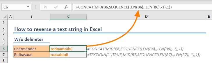
Reversing a text string without delimiters
In the following example:
- The LEN returns the number of characters for the string “Charizard” = 10
- The SEQUENCE returns an array of descending numbers starting from 10 = {10;9;8;7;6;5;4;3;2;1}
- The MID function return 1 character for each number in the array = {«r»;»e»;»d»;»n»;»a»;»m»;»r»;»a»;»h»;»C»}
- Finally, either the CONCAT or TEXTJOIN merges the characters in reverse order = rednamrahC
=CONCAT(MID(B6,SEQUENCE(LEN(B6),,LEN(B6),-1),1))
=TEXTJOIN(«»,TRUE,MID(B7,SEQUENCE(LEN(B7),,LEN(B7),-1),1))
Reversing a text string with delimiters
If you want to put a delimiter character(s) between each character of the source text, prefer using the TEXTJOIN function instead, and enter the delimiter into the first argument. For example, dots (.) separate each character in the following example.
=TEXTJOIN(«.»,TRUE,MID(B11,SEQUENCE(LEN(B11),,LEN(B11),-1),1))

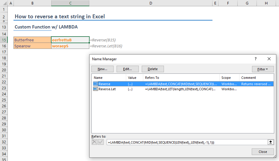
Bonus: A custom formula to reverse a text string in Excel
The LAMBDA function allows creating custom functions using other Excel formulas. Once you add the formula as a named range and you can start using the named range as your custom function. For detailed information please check out the LAMBDA page: Function: LAMBDA
=LAMBDA(text,CONCAT(MID(text,SEQUENCE(LEN(text),,LEN(text),-1),1)))
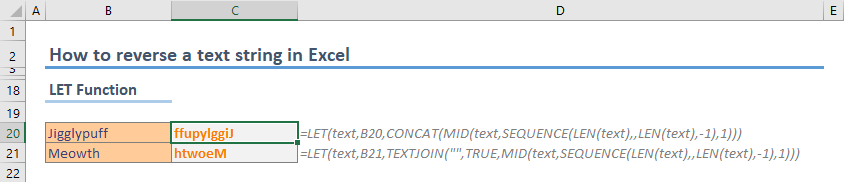
Simplify your functions using the LET Function
Additionally, you can check out the LET function to make your functions use a single argument. You can define in-formula named ranges to replace the actual references in the formula. In the following examples, the named range text is defined in the LET function to replace cell references:
=LET(text,B20,CONCAT(MID(text,SEQUENCE(LEN(text),,LEN(text),-1),1)))
=LET(text,B21,TEXTJOIN(«»,TRUE,MID(text,SEQUENCE(LEN(text),,LEN(text),-1),1)))
When copying this formula, only single reference needs to be changed instead of three.