
 Excel has some great functions available for working with long phrases (strings). It has RIGHT, LEFT, and TRIM to manage sub-strings. It also has FIND and SEARCH to look for specific characters or sub-strings inside a phrase. The only problem is that FIND and SEARCH look from left to right in a string. If you need to look for something starting at the end of a string, there isn’t a good tool built into Excel to do so. Fortunately, it is possible to build a formula to do just that – a reverse string search. Here’s how…
The Normal FIND Function
Let’s assume we have a simple string of characters we want to manipulate:
The quick brown fox jumps over the lazy dog.
If we were looking to identify the first word in the string, we could use a basic FIND function. The syntax for FIND is as follows:
=FIND(find_text, within_text, [start_num])
Assuming our string is in cell A1, the FIND function that locates the first space in the sentence is as follows:
=FIND(" ",A1)
The function returns 4. To get the first word in the sentence, we can use a LEFT function. The syntax for the LEFT function is as follows:
=LEFT(text, [num_chars])
The LEFT function that gives us the first word is as follows:
=LEFT(A1, FIND(" ",A1)-1)
It returns The. But what if we want the last word in the sentence? For that, we need to reverse the FIND function…
Get the latest Excel tips and tricks by joining the newsletter!
 Andrew Roberts has been solving business problems with Microsoft Excel for over a decade. Excel Tactics is dedicated to helping you master it.
Join the newsletter to stay on top of the latest articles. Sign up and you’ll get a free guide with 10 time-saving keyboard shortcuts!
Pages: 1 2 3 4
In this blog post we create a reverse FIND formula to extract text after the last occurrence of a character.
Many of you reading this may already be familiar with the FIND function. You would probably have used it with LEFT or MID to locate a delimiter character, and return text before, or after that character.
In this tutorial we want to extract text after the last occurrence of a character, so want to create a reverse find effect.
Watch the Video – Reverse Find Formula
In this example, we are working with the data below in column A. We wanted to extract the text after the final hyphen character.
Each cell contains a varying number of hyphens, so we need to identify the position of the last occurrence of the character, and then extract the text.
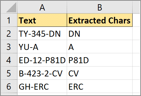
The completed Excel formula for this reverse string search is shown below.
=RIGHT(A2,LEN(A2)-FIND("*",SUBSTITUTE(A2,"-","*",LEN(A2)-LEN(SUBSTITUTE(A2,"-","")))))
This formula is a monster so a detailed explanation is shown below. The video above also explains it step by step.
Find the Total Occurrences of the Character
The first job on our hands is to return the total occurrences of the hyphen character.
Our ultimate aim is to retrieve some text after the last occurrence, so we need to know how many there are in total.
The formula below uses the SUBSTITUTE function to replace all occurrences of a hyphen with nothing. A LEN function is used to count the number of characters remaining when the hyphens are removed.
This value is subtracted from the total number of characters in the cell, leaving us with the answer to the total number of hyphens.
LEN(A2)-LEN(SUBSTITUTE(A2,"-",""))
Replace the Last Character with a Unique Marker
We will now replace the last occurrence of the hyphen with a unique character, which we can then use to easily extract the text we want.
An asterisk (*) has been used in this example as the unique marker. It could have been any text character.
The brilliant SUBSTITUTE function is used to accomplish this, with a little help from some friends.
The previous part of the formula has been used in the instance number argument of the SUBSTITUTE function, to specify to replace the last hyphen.
SUBSTITUTE(A2,"-","*",LEN(A2)-LEN(SUBSTITUTE(A2,"-","")))
Extract the Text after the Final Delimiter Character
Now that we have inserted a unique marker in the position of the final delimiter character, it is time to find it and extract the text we want.
The following formula was added to what we have from the previous step. The ??? represents the formula part from the previous step.
=RIGHT(A2,LEN(A2)-FIND("*",???))
The RIGHT function is used to extract text from the end of cell A2.
To calculate the number of characters to extract, the LEN function returns the total characters in the cell. And then the FIND function locates our unique marker character.
The position of the marker character is subtracted from the total characters in the cell.
The final formula is as below.
=RIGHT(A2,LEN(A2)-FIND("*",SUBSTITUTE(A2,"-","*",LEN(A2)-LEN(SUBSTITUTE(A2,"-","")))))
This can be adjusted to return text from the second from last delimiter, or anything you want really.
You now have a way of searching a string from right-to-left, in addition to the typical left-to-right search.
Related Excel Formula Tutorials
- How to use the TEXT function of Excel – with examples
- Extract the postcode from a UK address
- 4 amazing tips for the CONCATENATE function
- 4 ways to separate text in Excel
This one is tested and does work (based on Brad’s original post):
=RIGHT(A1,LEN(A1)-FIND("|",SUBSTITUTE(A1," ","|",
     LEN(A1)-LEN(SUBSTITUTE(A1," ","")))))
If your original strings could contain a pipe «|» character, then replace both in the above with some other character that won’t appear in your source. (I suspect Brad’s original was broken because an unprintable character was removed in the translation).
Bonus: How it works (from right to left):
LEN(A1)-LEN(SUBSTITUTE(A1," ","")) – Count of spaces in the original string
SUBSTITUTE(A1," ","|", ... ) – Replaces just the final space with a |
FIND("|", ... ) – Finds the absolute position of that replaced | (that was the final space)
Right(A1,LEN(A1) - ... )) – Returns all characters after that |
EDIT: to account for the case where the source text contains no spaces, add the following to the beginning of the formula:
=IF(ISERROR(FIND(" ",A1)),A1, ... )
making the entire formula now:
=IF(ISERROR(FIND(" ",A1)),A1, RIGHT(A1,LEN(A1) - FIND("|",
    SUBSTITUTE(A1," ","|",LEN(A1)-LEN(SUBSTITUTE(A1," ",""))))))
Or you can use the =IF(COUNTIF(A1,"* *") syntax of the other version.
When the original string might contain a space at the last position add a trim function while counting all the spaces: Making the function the following:
=IF(ISERROR(FIND(" ",B2)),B2, RIGHT(B2,LEN(B2) - FIND("|",
    SUBSTITUTE(B2," ","|",LEN(TRIM(B2))-LEN(SUBSTITUTE(B2," ",""))))))
This tutorial talks about how to reverse search in Excel. There are two different methods to do this that I will explain in this tutorial. The methods use different formulas to do the same. One of these methods uses VBA code, while the other method makes use of the built-in Excel functions. Both the methods make it pretty easy to do a reverse string search in Excel.
Reverse searching can be a useful technique in case you want to find the position of a certain character or word from the end of a string. As Excel does not have any native formula to do that, so you will have to do it by yourself. Using the methods explained below, you can easily perform searches from the end of a string in Excel.
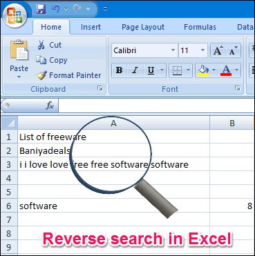
Searching in MS Excel files is nothing new, there are already some add-ins to search and find in Excel sheets. But the search offered by them is a straight search; it cannot search in the reverse direction. That’s why I have listed the following methods to perform a reverse search in Excel.
As I said above, there are two different methods that I will use to perform a reverse search in Excel. In the first method I will use a user defined function that is written in VBA. And I will use some built-in functions of Excel in the second formula to do the same. Let’s have a look at them one by one.
Method 1: Reverse String Search in Excel Using VBA:
In this method I will show you how to perform reverse searches in Excel to find the position a certain character or a word from the end of a string. In this formula I will use a user defined function ReverseSearch, written in VBA whose syntax and code is given below. This formula receives two parameters, one for the source string and second for the word that is to be searched. After that it returns the position of the first character of the specified word from the end of the string.
ReverseSearch(Text_String, Word_to_Find)
See its VBA code here:
Public Function ReverseSearch(strBase As String, strTerm As String) As Integer

'Purpose: Returns the position of string from the end

Dim x As Integer

On Error GoTo ErrorMessage

If strTerm = "" Then

ReverseSearch = 0

Else

x = Len(strTerm)

ReverseSearch = InStr(StrReverse(strBase), StrReverse(strTerm))

ReverseSearch = (ReverseSearch + x) - 1

End If

Exit Function

ErrorMessage:

MsgBox "There seems to be an error."

End

End Function
You have to put the above code in VBA module of Excel. For that, click Alt+F11. In the window that opens up, right click on name of your Excel, click on Insert > Module. In the window that opens up, paste the entire VBA code I have given above. Then click on Save, and save the Excel as “Excel Macro-Enabled Workbook .xlsm” file. Then close the macro window.
Now, you can use the formula (that I highlighted in Red above) to do reverse search in Excel. You can see the below screenshot, showing the working of this formula.
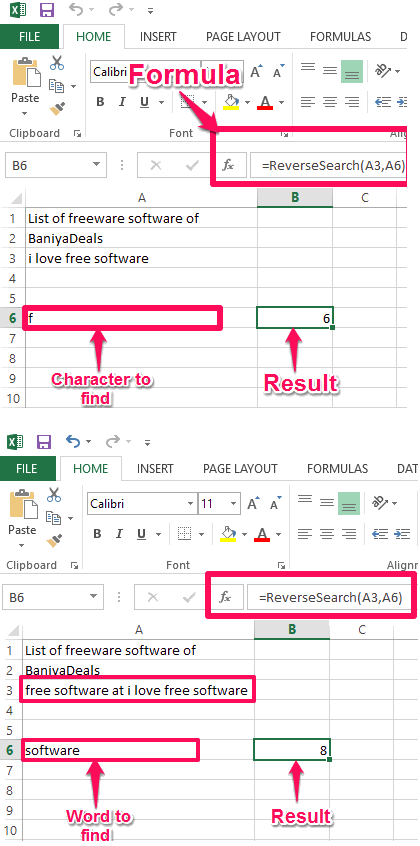
In the above screenshot I have used this formula to find the position of a certain character from the end of the string. And also, I have used it to find the position of a specified word. You can see that it has resulted in the correct position of the specified word and character in both the cases.
This is a very simple method to do reverse search in Excel, as you just need to paste the VBA code, and then you can do as many reverse searches as you want. Just paste the VBA code once in the Excel macros and then you can use it anytime unless, you remove Excel from your PC.
Method 2: Reverse String Search in Excel Using Excel Functions:
In the above method I explained how to reverse search using VBA. Now, if you don’t want to use VBA functions or you find it difficult to use them in Excel, then there is another function that can do it for you. Using the built-in functions of Excel I have made another formula that can do reverse search in Excel. Though it’s a little bit tricky, but once you understand its functionality, then I am sure that you will like it. The syntax of this formula is given below.
LEN(Text_String) – SEARCH(“^^^”, SUBSTITUTE(Text_String, Word_to_Find, “^^^”, (LEN(Text_String)-LEN(SUBSTITUTE(Text_String,Word_to_Find, “”)))/LEN(Word_to_Find))) + 1
This formula uses Search, Substitute, and Len functions of Excel to do Reverse string search.
The way this formula works is that it finds the last instance of the specified substring and then replaces it with “^^^”, and returns its index. And after that, obtained index is subtracted from the length of the source string to get its position from the end. However, if your source string contains the sequence “^^^”, then this formula will fail and you will need to replace “^^^” in above formula to some other string (that doesn’t exist in your text).
After using this formula, you can easily find the position of a word from its first occurrence in the source string from the end. You can see the working of the formula in the following screenshot.
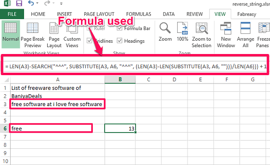
Now, after seeing this screenshot, you will get the idea how this formula works to find the position of certain word using the reverse search technique in Excel. Do note that this formula is made by using the built-in excel functions. So, if you don’t want to use an external formula written in VBA, then you may give this a try.
In this way you can perform a reverse search in Excel using this simple formula. Based on your needs, you can search a particular character or a word in your source string in your worksheet.
Also see: How to do Reverse vLookup in Excel.
My Final Verdict
There have been a lot of times when I had to do reverse string search in Excel. The first time I had to do I was very surprised to know that Excel does not provide any functionality to do reverse string search in Excel. And when I started looking for a solution, I wasn’t able to find any easy one.
Now, I have provided 2 solutions to you to do reverse string search in Excel. Both work equally well, and both give correct results. I personally prefer the VBA code, because it is simple to use. But if you want to stick to core Excel functions, then the second method works equally well.
In case you know some other ways to do reverse string search in Excel, do let me know in comments below.
How do you reverse find in Excel?
In this tutorial we want to extract text after the last occurrence of a character, so want to create a reverse find effect.
- Watch the Video.
- The Reverse FIND Excel Formula.
- Find the Total Occurrences of the Character.
- Replace the Last Character with a Unique Marker.
- Extract the Text after the Final Delimiter Character.
How do I Vlookup from right to left?
The VLOOKUP function only looks to the right. To look up a value in any column and return the corresponding value to the left, simply use INDEX and MATCH.
How do I search for text to the left of a character in Excel?
To extract the leftmost characters from a string, use the LEFT function in Excel. To extract a substring (of any length) before the dash, add the FIND function. Explanation: the FIND function finds the position of the dash. Subtract 1 from this result to extract the correct number of leftmost characters.
How do I extract left text in Excel?
FIND returns the position (as a number) of the first occurrence of a space character in the text. This position, minus one, is fed into the LEFT function as num_chars. The LEFT function then extracts characters starting at the the left side of the text, up to (position – 1).
How do I pull a character out of a cell in Excel?
Extract text from a cell in Excel
- =RIGHT(text, number of characters)
- =LEFT(text, number of characters)
- =MID(text,start_num,num_chars)
What is rept Excel?
The Excel REPT function repeats characters a given number of times. For example, =REPT(“x”,5) returns “xxxxx”. number_times – The number of times to repeat text.
What is function rept?
The REPT Function is categorized under Excel Logical functions. The function will repeat characters a given number of times. In financial analysis. This guide will teach you to perform financial statement analysis of the income statement,, we can use the REPT function to fill a cell or pad values to a certain length.
What is right and left function in Excel?
The LEFT and RIGHT functions are used to return characters from the start or end of a string. The following explains how to select these functions and some possible uses. This feature works the same in all modern versions of Microsoft Excel: 2010, 2013, and 2016. To use the LEFT and RIGHT functions in Excel:
How do you use the right formula in Excel?
1. Show Formulas option on the Excel ribbon. In your Excel worksheet, go to the Formulas tab > Formula Auditing group and click the Show Formulas button. Microsoft Excel displays formulas in cells instead of their results right away. To get the calculated values back, click the Show Formulas button again to toggle it off.
How do you use right function in Excel?
To use the LEFT and RIGHT functions in Excel: On the Formulas tab, in the Function Library group, click the Insert Function command. In the Insert Function dialog box: Search on “LEFT” or “RIGHT” or, in the Or select a category drop-down box, select Text. Under Select a function, select LEFT or RIGHT.
How do you use search in Excel?
Hit the key combination Ctrl + F on your keyboard. Type in the words you want to find. Enter the exact word or phrase you want to search for, and click on the “Find” button in the lower right of the Find window. Excel will begin searching for matches of the word, or words, you entered in the search field.
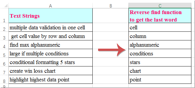
Generally, when we try to find a particular sentence, we always try to find it by using the first words of the text, but if we clearly understand the data, we can see most of the sentences will start with the same words, but they always end with different words. So, by searching for sentences using the last words rather than the first words, we can return fewer results than if we used the first words. So, we can list the last words of the sentences using this process.
Read this tutorial to learn how you can apply the Reverse Find or Search function in Excel. This process uses the formulas supported by Excel to complete the task. The keywords in the formula are «trim» and «substitute».
Applying the Reverse Find or Search Function Using Formula
Here, we will first get the first result using the formula, then use the auto-fill handle to get all the results. Let us see a simple process to apply the reverse find or search function using the formulas in Excel in a fast and efficient way.
Step 1
Let us consider an Excel sheet where the data present in the sheet is similar to the data present in the below screen shot.

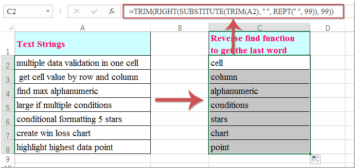
Now click on an empty cell, which will be cell C2 in our case, and enter the formula as =TRIM(RIGHT(SUBSTITUTE(TRIM(A1), » «, REPT(» «, 99)), 99)) in the formula box and hit the «Enter» button to get the first result, as shown in the below image.

Step 2
As we can see, we have achieved the first result. We can get all the other results by dragging down from the right corner of the first result.

Conclusion
In this tutorial, we used a simple example to demonstrate how we can apply the Reverse Find or Search function in Excel to highlight a particular set of data.
Как правило, мы можем применить функцию поиска или поиска для поиска определенного текста слева направо в текстовой строке по определенному разделителю. Если вам нужно отменить функцию поиска, чтобы найти слово, начинающееся в конце строки, как показано на следующем снимке экрана, как вы могли бы это сделать?
Примените функцию обратного поиска, чтобы искать слово справа в текстовой строке с формулой
Примените функцию обратного поиска, чтобы искать слово справа в текстовой строке с формулой
Чтобы получить последнее слово справа в текстовой строке, вам может помочь следующая формула, сделайте следующее:
Введите эту формулу: = ОБРЕЗАТЬ (ПРАВО (ПОДСТАВИТЬ (ОБРЕЗАТЬ (A2); «»; ПОВТОР («»; 99)); 99)) в пустую ячейку, а затем перетащите дескриптор заполнения вниз к ячейкам, из которых вы хотите извлечь последнее слово, и все последнее слово в текстовых строках было отображено сразу, см. снимок экрана:
Внимание: Формула может найти слово только справа на основе разделителя пробела.
Лучшие инструменты для работы в офисе
Kutools for Excel Решит большинство ваших проблем и повысит вашу производительность на 80%
- Снова использовать: Быстро вставить сложные формулы, диаграммы и все, что вы использовали раньше; Зашифровать ячейки с паролем; Создать список рассылки и отправлять электронные письма …
- Бар Супер Формулы (легко редактировать несколько строк текста и формул); Макет для чтения (легко читать и редактировать большое количество ячеек); Вставить в отфильтрованный диапазон…
- Объединить ячейки / строки / столбцы без потери данных; Разделить содержимое ячеек; Объединить повторяющиеся строки / столбцы… Предотвращение дублирования ячеек; Сравнить диапазоны…
- Выберите Дубликат или Уникальный Ряды; Выбрать пустые строки (все ячейки пустые); Супер находка и нечеткая находка во многих рабочих тетрадях; Случайный выбор …
- Точная копия Несколько ячеек без изменения ссылки на формулу; Автоматическое создание ссылок на несколько листов; Вставить пули, Флажки и многое другое …
- Извлечь текст, Добавить текст, Удалить по позиции, Удалить пробел; Создание и печать промежуточных итогов по страницам; Преобразование содержимого ячеек в комментарии…
- Суперфильтр (сохранять и применять схемы фильтров к другим листам); Расширенная сортировка по месяцам / неделям / дням, периодичности и др .; Специальный фильтр жирным, курсивом …
- Комбинируйте книги и рабочие листы; Объединить таблицы на основе ключевых столбцов; Разделить данные на несколько листов; Пакетное преобразование xls, xlsx и PDF…
- Более 300 мощных функций. Поддерживает Office/Excel 2007-2021 и 365. Поддерживает все языки. Простое развертывание на вашем предприятии или в организации. Полнофункциональная 30-дневная бесплатная пробная версия. 60-дневная гарантия возврата денег.
")
Вкладка Office: интерфейс с вкладками в Office и упрощение работы
- Включение редактирования и чтения с вкладками в Word, Excel, PowerPoint, Издатель, доступ, Visio и проект.
- Открывайте и создавайте несколько документов на новых вкладках одного окна, а не в новых окнах.
- Повышает вашу продуктивность на 50% и сокращает количество щелчков мышью на сотни каждый день!
")
Комментарии (0)
Оценок пока нет. Оцените первым!
In my research and tutoring excel, I have found that many people find the Reverse lookup concept to be among the top 10 complicated things in excel. This article hopes to shed more light than heat in demystifying the Reverse Lookup in excel.
In the normal lookup, we use the Column and/or Row header to return the value that falls in the intersection. But in the reverse lookup, we shall use the value to return the column and/or row header
For example, say you have below appointments Calendar and you want to lookup & return the scheduled date & time for customer Joy Bell

There are 4 ways to carry out this kind of a Reverse Lookup;
-
USING INDEX & SUMPRODUCT
=INDEX(D3:G3,0,
   SUMPRODUCT(--(D4:G14=I3)*(COLUMN(D3:G3)-COLUMN(D3)+1)))
+INDEX(C4:C14,
  SUMPRODUCT(--(D4:G14=I3)*(ROW(C4:C14)-ROW(C4)+1)))
How it works:
The trick is to break down the formula into small parts;
- INDEX(D3:G3,0,SUMPRODUCT(–(D4:G14=I3)*(COLUMN(D3:G3)-COLUMN(D3)+1))) this is the part that looks up the Date values in the columns
►SUMPRODUCT(–(D4:G14=I3)*(COLUMN(D3:G3)-COLUMN(D3)+1)) returns a column number given a criteria i.e.
- – -(D4: G14=I3) →returns an array of 1 & 0. 1 represents where the criterion is met
{0,0,0,0;0,0,0,0;0,0,0,0;0,0,0,0;0,0,1,0;
0,0,0,0;0,0,0,0;0,0,0,0;0,0,0,0;0,0,0,0;0,0,0,0}
- (COLUMN(D3: G3)-COLUMN(D3)+1)→ returns an array of relative positions of the columns
{1,2,3,4}
SUMPRODUCT takes up the 2 arrays and using the techniques of conjunction truth table returns 3
►INDEX(D3:E3,0,3) returns the value in column 3 given the range D3:E3= 13-05-2016
2. INDEX(C4:C14,SUMPRODUCT(–(D4:G14=I3)*(ROW(C4:C14)-ROW(C4)+1))) this is the part that looks up the Time values in the rows.
The breakdown of the formula is the same as explained above other than INDEX looks up the rows instead of columns.
When you combine the two parts you form a DateTime Value which you can custom format to fit.
=INDEX(D3:E3,0,3)+INDEX(C4:C14,5) = 13-05-2016 12:00:00 PM
2.Using an Array Formula (INDEX & MAX)
{=INDEX(D3:G3,
  MAX((D4:G14=I7)*(COLUMN(D3:G3)-COLUMN(D3)+1)))
+INDEX(C4:C14,
  MAX((D4:G14=I7)*(ROW(C4:C14)-ROW(C4)+1)))}
How it works:
- =INDEX(D3: G3,MAX((D4: G14=I7)*(COLUMN(D3: G3)-COLUMN(D3)+1))) like in the SUMPRODUCT formula, this is the part that looks up the Date Value
►(D4: G14=I7)*(COLUMN(D3: G3)-COLUMN(D3)+1) this part generates an array of Column number where the criteria are met and zero for the rest.
{0,0,0,0;0,0,0,0;0,0,0,0;0,0,0,0;0,0,3,0
;0,0,0,0;0,0,0,0;0,0,0,0;0,0,0,0;0,0,0,0;0,0,0,0}
►MAX function returns the maximum number in the array
MAX({0,0,0,0;0,0,0,0;0,0,0,0;0,0,0,0;0,0,3,0
;0,0,0,0;0,0,0,0;0,0,0,0;0,0,0,0;0,0,0,0;0,0,0,0})=3
►INDEX(D3:E3,0,3) returns the Date Value.
- INDEX(C4:C14,MAX((D4:G14=I7)*(ROW(C4:C14)-ROW(C4)+1))) this generates the Time Value
The same breakdown works with the Time Value.
NB: This is an Array formula so remember to Ctrl + Shift +Enter
3. Using Array Formula (SMALL & IF)
{=SMALL(
   IF(D4:G14=I10,(D3:G3+C4:C14))
,1)}
This is the shortest and easiest to understand.
First, you need to understand how Excel stores date and time i.e. dates as serial numbers and time as a fractional portion of a 24 hour day.
Secondly, you need to understand that a DateTime Value is just a sum of this Date serial Number and fractional Time Value.
►(D3:G3+C4: C14) returns a two-dimensional array of DateTime Value
{42501.3333333333,42502.3333333333,42503.3333333333,42504.3333333333;
42501.375,42502.375,42503.375,42504.375;42501.4166666667,42502.4166666667,
42503.4166666667,42504.4166666667;42501.4583333333,42502.4583333333,
42503.4583333333,42504.4583333333;42501.5,42502.5,42503.5,42504.5;
42501.5416666667,42502.5416666667,42503.5416666667,42504.5416666667;
42501.5833333333,42502.5833333333,42503.5833333333,42504.5833333333;
42501.625,42502.625,42503.625,42504.625;42501.6666666667,42502.6666666667,
42503.6666666667,42504.6666666667;42501.7083333333,42502.7083333333,
42503.7083333333,42504.7083333333;42501.75,42502.75,42503.75,42504.75}
►IF(D4: G14=I10,(D3:G3+C4: C14)) returns an array of the DateTime value that meets the criteria
{FALSE,FALSE,FALSE,FALSE;FALSE,FALSE,FALSE,FALSE;FALSE,FALSE,FALSE,
FALSE;FALSE,FALSE,FALSE,FALSE;FALSE,FALSE,42503.5,FALSE;FALSE,FALSE,
FALSE,FALSE;FALSE,FALSE,FALSE,FALSE;FALSE,FALSE,FALSE,FALSE;FALSE,FALSE,
FALSE,FALSE;FALSE,FALSE,FALSE,FALSE;FALSE,FALSE,FALSE,FALSE}
►SMALL returns the first smallest number in the array =42503.5
►Format the number “dd-mm-yyyy h:mm AM/PM” = 13-05-2016 12:00PM
4. Using AGGREGATE
Other than INDEX & SUMPRODUCT combination this is the other NON-Array formula you can use to do this Reverse lookup
=AGGREGATE(15,6,((D3:G3+C4:C14)/(D4:G14=I14)),1)
How it works;
Watch these Videos on the AGGREGATE Function.
DOWNLOAD WORKSHEET
RELATED ARTICLES:
2 WAY LOOKUP IN EXCEL
LOOKUP AND SUM IN EXCEL
![]()
Excel VBA Course — From Beginner to Expert
200+ Video Lessons
50+ Hours of Instruction
200+ Excel Guides
Become a master of VBA and Macros in Excel and learn how to automate all of your tasks in Excel with this online course. (No VBA experience required.)
View Course
Subscribe for Weekly Tutorials
BONUS: subscribe now to download our Top Tutorials Ebook!
![]()
Excel VBA Course — From Beginner to Expert
200+ Video Lessons
50+ Hours of Video
200+ Excel Guides
Become a master of VBA and Macros in Excel and learn how to automate all of your tasks in Excel with this online course. (No VBA experience required.)
View Course