
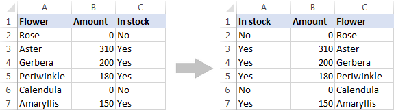
Sometimes, you may have a need to flip the data in Excel, i.e., to reverse the order of the data upside down in a vertical dataset and left to right in a horizontal dataset.
Now, if you’re thinking that there must be an inbuilt feature to do this in Excel, I’m afraid you’d be disappointed.
While there are multiple ways you can flip the data in Excel, there is no inbuilt feature. But you can easily do this using simple a sorting trick, formulas, or VBA.
In this tutorial, I will show you how to flip the data in rows, columns, and tables in Excel.
So let’s get started!
Flip Data Using SORT and Helper Column
One of the easiest ways to reverse the order of the data in Excel would be to use a helper column and then use that helper column to sort the data.
Flip the Data Vertically (Reverse Order Upside Down)
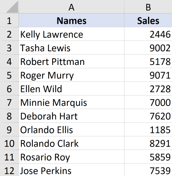
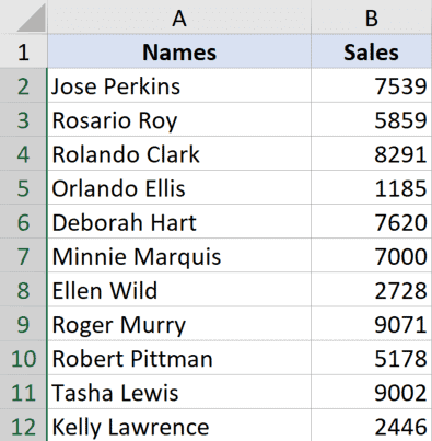
Suppose you have a data set of names in a column as shown below and you want to flip this data:

Below are the steps to flip the data vertically:
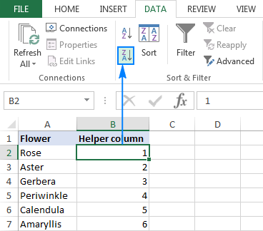
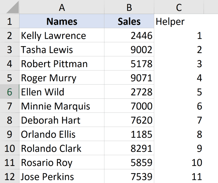
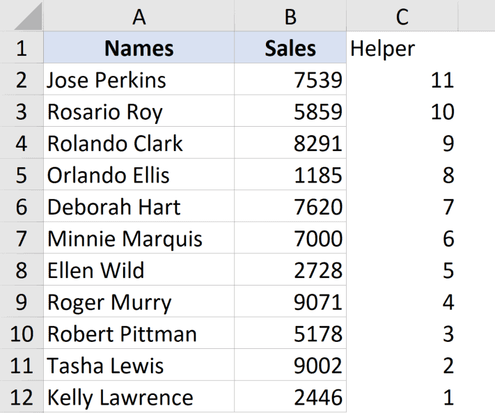
- In the adjacent column, enter ‘Helper’ as the heading for the column
- In the helper column, enter a series of numbers (1,2,3, and so on). You can use the methods shown here to do this quickly

- Select the entire data set including the helper column
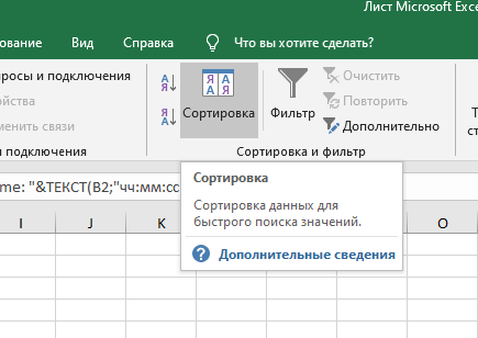
- Click the Data tab

- Click on the Sort icon

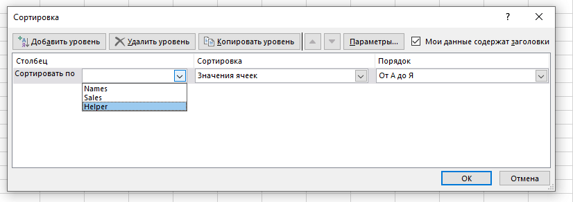
- In the Sort dialog box, select ‘Helper’ in the ‘Sort by’ dropdown

- In the Order drop-down, select ‘Largest to Smallest’
- Click OK


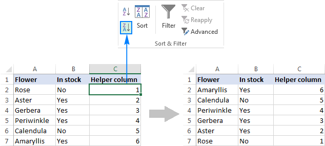
The above steps would sort the data based on the helper column values, which would also lead to reversing the order of the names in the data.

Once done, feel free to delete the helper column.
In this example, I’ve shown you how to flip the data when you just have one column, but you can also use the same technique if you have an entire table. Just make sure that you select the entire table and then use the helper column to sort the data in descending order.
Flip the Data Horizontally
You can also follow the same methodology to flip the data horizontally in Excel.
Excel has an option to sort the data horizontally using the Sort dialog box (the ‘Sort left to right’ feature).
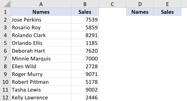
Suppose you have a table as shown below and you want to flip this data horizontally.

Below are the steps to do this:
- In the row below, enter ‘Helper’ as the heading for the row
- In the helper row, enter a series of numbers (1,2,3, and so on).

- Select the entire data set including the helper row
- Click the Data tab
- Click on the Sort icon
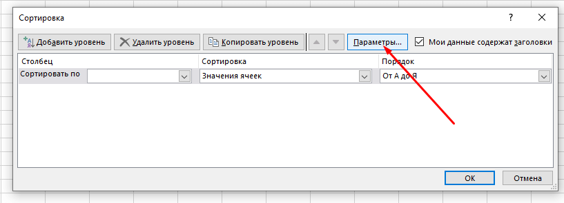
- In the Sort dialog box, click on the Options button.

- In the dialog box that opens, click on ‘Sort left to right’

- Click OK
- In the Sort by drop-down, select Row 3 (or whatever row has your helper column)
- In the Order drop-down, select ‘Largest to Smallest’
- Click OK


The above steps would flip the entire table horizontally.

Once done, you can remove the helper row.
Flip Data Using Formulas
Microsoft 365 has got some new formulas that make it really easy to reverse the order of a column or a table in Excel.
In this section, I’ll show you how to do this using the SORTBY formula (if you’re using Microsoft 365), or the INDEX formula (if you’re not using Microsoft 365)
Using the SORTBY function (available in Microsoft 365)
Suppose you have a table as shown below and you want to flip the data in this table:

To do this, first, copy the headers and place them where you would want the flipped table

Now, use the following formula below the cell in the left-most header:
=SORTBY($A$2:$B$12,ROW(A2:A12),-1)
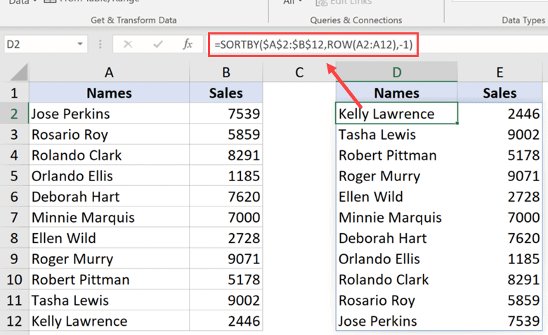
The above formula sorts the data and by using the result of the ROW function as the basis to sort it.
The ROW function in this case would return an array of numbers that represents the row numbers in between the specified range (which in this example would be a series of numbers such as 2, 3, 4, and so on).
And since the third argument of this formula is -1, it would force the formula to sort the data in descending order.
The record that has the highest row number would come at the top and the one which has the lowest rule number would go at the bottom, essentially reversing the order of the data.
Once done, you can convert the formula to values to get a static table.
Using the INDEX Function
In case you don’t have access to the SORTBY function, worry not – you can use the amazing INDEX function.
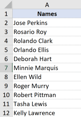
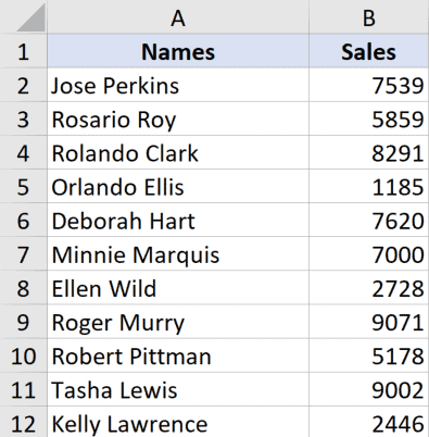
Suppose you have a dataset of names as shown below and you want to flip this data.

Below is the formula to do this:
=INDEX($A$2:$A$12,ROWS(A2:$A$12))

How does this formula work?
The above formula uses the INDEX function that would return the value from the cell based on the number specified in the second argument.
The real magic happens in the second argument where I have used the ROWS function.
Since I have locked the second part of the reference in the ROWS function, in the first cell, it would return the number of rows between A2 and A12, which would be 11.
But when it goes down the rows, the first reference would change to A3, and then A4, and so on, while the second reference would remain as is because I have locked it and made it absolute.
As we go down the rows, the result of the ROWS function would decrease by 1, from 11 to 10 to 9, and so on.
And since the INDEX function returns us the value based on the number in the second argument, this would ultimately give us the data in the reverse order.
You can use the same formula even if you have multiple columns in the data set. however, you will have to specify a second argument that would specify the column number from which the data needs to be fetched.
Suppose you have a data set as shown below and you want to reverse the order of the entire table:

Below is the formula that will do that for you:
=INDEX($A$2:$B$12,ROWS(A2:$A$12),COLUMNS($A$2:A2))

This is a similar formula where I’ve also added a third argument that specifies the column number from which the value should be fetched.
To make this formula dynamic, I have used the COLUMNS function that would keep on changing the column value from 1 to 2 to 3 as you copy it to the right.
Once done, you can convert the formulas to values to make sure that you have a static result.
Note: When you use a formula to reverse the order of a data set in Excel, it would not retain the original formatting. If you need the original formatting on the sorted data as well, you can either apply it manually or copy and paste the formatting from the original data set to the new sorted dataset
Flip Data Using VBA
If flipping the data in Excel is something you have to do quite often, you can also try the VBA method.
With a VBA macro code, you can copy and paste it once within the workbook in the VBA editor, and then reuse it over and over again in the same workbook.
You can also save the code in the Personal Macro Workbook or as an Excel add-in and be able to use it in any workbook on your system.
Below is the VBA code that would flip the selected data vertically in the worksheet.
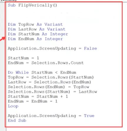
Sub FlipVerically()

'Code by Sumit Bansal from TrumpExcel.com

Dim TopRow As Variant
Dim LastRow As Variant
Dim StartNum As Integer
Dim EndNum As Integer

Application.ScreenUpdating = False

StartNum = 1
EndNum = Selection.Rows.Count

Do While StartNum < EndNum
TopRow = Selection.Rows(StartNum)
LastRow = Selection.Rows(EndNum)
Selection.Rows(EndNum) = TopRow
Selection.Rows(StartNum) = LastRowStartNum = StartNum + 1
EndNum = EndNum - 1
Loop

Application.ScreenUpdating = True
End Sub
To use this code, you first need to make the selection of the data set that you want to reverse (excluding the headers), and then run this code.
How does this code work?
The above code first counts the total number of rows in the data set and assigns that to the variable EndNum.
It then uses the Do While loop where the sorting of the data happens.
The way it sorts this data is by taking the first and the last row and swapping these. It then moves to the 2nd row in the second last row and then swaps these. Then it moves to the third row in the third last row and so on.
The loop ends when all the sorting is done.
It also uses the Application.ScreenUpdating property and sets it to FALSE while running the code, and then turn it back to TRUE when the code has completed running.
This ensures that you don’t see the changes happening in real-time on your screen it also speeds up the process.
How to use the Code?
Follow the below steps to copy and paste this code in the VB Editor:
- Open the Excel file where you want to add the VBA code
- Hold the ALT key and press the F-11 key (you can also go to the Developer tab and click on the Visual Basic icon)
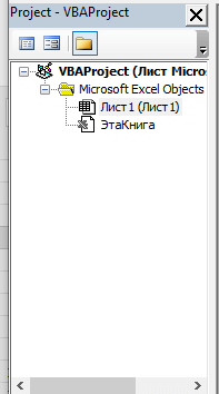
- In the Visual Basic Editor that opens up, there would be a Project Explorer on the left part of the VBA editor. If you don’t see it, click on the ‘View’ tab and then click on ‘Project Explorer’

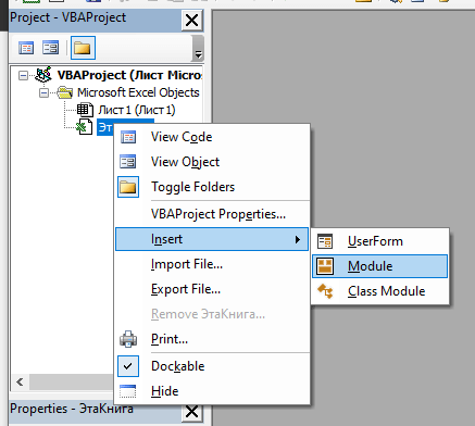
- Right-click on any of the objects for the workbook in which you want to add the code
- Go to the Insert option and then click on Module. This will add a new module to the workbook

- Double-click on the module icon in the Project Explorer. This will open the code window for that module
- Copy and paste the above VBA code into the code window


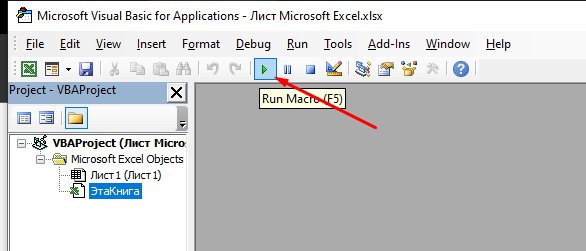
To run the VBA macro code, first select the dataset that you want to flip (excluding the headers).
With the data selected, go to the VB Editor and click on the green play button in the toolbar, or select any line in the code and then hit the F5 key

So these are some of the methods you can use to flip the data in Excel (i.e., reverse the order of the data set).
All the methods that I have covered in this tutorial (formulas, SORT feature, and VBA), can be used to flip the data vertically and horizontally (you’ll have to adjust the formula and VBA code accordingly for horizontal data flipping).
I hope you found this tutorial useful.
Other Excel tutorials you may also like:
- How to Sort by the Last Name in Excel (Easy Guide)
- How to Sort By Color in Excel (in less than 10 seconds)
- How to Sort Worksheets in Excel using VBA (alphabetically)
- How to do a Multiple Level Data Sorting in Excel
Excel Reverse Order (Table of Contents)
- Introduction to Excel Reverse Order
- Methods to Reverse Column Order
Introduction to Excel Reverse Order
Reversing the order is nothing but flipping the column values; this means the last value in your column should be the first value in reversed order and the second last should be the second value and going on, the first value should be the one that gets entered at last in a reversed column. Well, it seems to be a pretty simple one-click task when you hear it out at first. However, it is not. Because there is no one-click button in Excel that does this task for you, besides it is really very hard to use the traditional Sort function as it only can sort the values based on the sorting order alphabetically or numerically and not with the flipping preferences. However, these are not the only, and you may come up with some creativity, your own ways to get the task done.
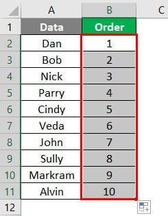
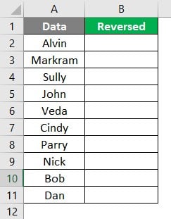
Let us see different methods that can be used to reverse the column order. Suppose we have data as shown below:
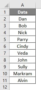
Column A consists of data, as you can see, that is not sorted. Here, we wanted the order to be reversed (column flip) in a way that Dan should appear first in a Reversed column and then Bob and likewise, Alvin should come as last in a Reversed column.
Methods to Reverse Column Order
Let’s understand the techniques to Reverse Column Order with a few methods.
You can download this Reverse Order Excel Template here – Reverse Order Excel Template
Methods #1 – Conventional Sort Method
Step 1: Add a column named Order after column A (Data) and try typing the numbers starting from 1,2. These numbers will be the order references for data values under column A.
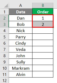
Step 2: Now, select the first two cells in the column named Order (column B) and then drag it down until B11 to get the sequential numbers from 1 to 10 across B1:B11.
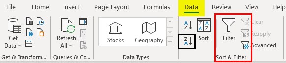
Step 3: Select the entire column B Data (B1:B11) and navigate to the Data tab in the Excel Ribbon. Within the Data tab, under the Sort & Filter group, click on the Sort Z to A (Highest to Lowest) button.
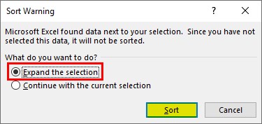
Step 4: As soon as you click on the Sort Z to A button, you’ll get a warning message from the function. As shown below. Don’t change anything in the default selection in that message box and click on the Sort button.
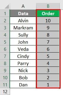
As soon as you click on the Sort button, you could see that the data has been sorted based on column B (named Order) values as Largest to Smallest and accordingly, column A values have also changed their places. Now, you can see Dan as the first entry in column A, Bob as second and going on, Alvin as the last entry.
This is one way to reverse the order of a column or flip the column.
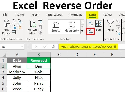
Methods #2 – Using Excel Formula
You can see that column A consists of all the names starting from Alvin up to Dan. Now, column B, named Reversed, is something where we will be adding a generic formula that can look up and add the values as flipped from column A. Which means the sequence will be Dan as first, Bob as second and going so on, Alvin will be the last entry under column B.
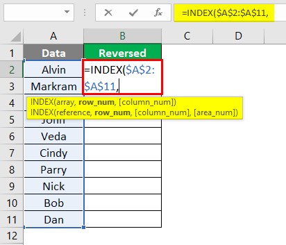
Step 1: In cell B2, start typing the INDEX formula and use $A2:$A$11 as an absolute reference to it (hit keyboard F4 button once to convert the reference into an absolute one).
Step 2: Now, use the ROWS function to add the relative row references. Use the same data reference inside the ROWS function (A2:A$11); however, this time, use F4 to make A11 as absolute.
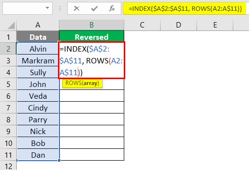
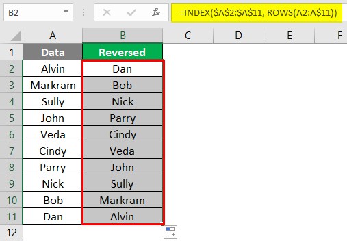
Step 3: Add two closing parentheses for ROWS as well as the INDEX function, and this formula is complete. You can press the Enter key as well as drag this formula across B2:B11 to get the desired result.
Things to Remember About Excel Reverse Order
- Excel doesn’t have any built-in function that reverses/flips the column order. It can be achieved with different formulae and their combinations.
- Excel SORT seems to be the best, simple yet faster way to achieve the order reversal or order flipping of a column.
- However, at the same time, using a combination of INDEX and ROWS function is more generic since it doesn’t alter the original order preference, and you still can have your values in original order if you changed your mind from flipping the column order.
Recommended Articles
This is a guide to Excel Reverse Order. Here we discuss How to Reverse Column Order in Excel along with practical examples and a downloadable excel template. You can also go through our other suggested articles –
- Trunc in Excel
- Compare Two Lists in Excel
- Logical Functions in Excel
- Sort Column in Excel
Flip a column of data order in Excel with Sort command
- Insert a series of sequence numbers besides the column.
- Click the Data > Sort Z to A, see screenshot:
- In the Sort Warning dialog box, check the Expand the selection option, and click the Sort button.
- Then you will see the number order of Column A is flipped.
Contents
- 1 How do I invert two columns in Excel?
- 2 How does a Vlookup work?
- 3 How do you swap two cells in an Excel spreadsheet?
- 4 How do you switch columns in docs?
- 5 How do I move columns in Excel?
- 6 How do you do a VLOOKUP for beginners?
- 7 Why is VLOOKUP so important?
- 8 What is an Xlookup in Excel?
- 9 How do you swap rows in sheets?
- 10 How do I switch between columns in Word?
- 11 How do you go back to 1 column in Google Docs?
- 12 How do I move columns to columns in Google Docs?
How do I invert two columns in Excel?
Press and hold the Shift key, and then drag the column to a new location. You will see a faint “I” bar along the entire length of the column and a box indicating where the new column will be moved. That’s it! Release the mouse button, then leave the Shift key and find the column moved to a new position.
How does a Vlookup work?
The VLOOKUP function performs a vertical lookup by searching for a value in the first column of a table and returning the value in the same row in the index_number position. The VLOOKUP function is a built-in function in Excel that is categorized as a Lookup/Reference Function.
How do you swap two cells in an Excel spreadsheet?
Click the More (…) button at the top right of Power Tools. Select the Flip adjacent cells, rows, and columns option. Then select the Flip entire columns option to swap the cells in the non-adjacent columns around.
How do you switch columns in docs?
How to Switch Between Columns in Google Docs (Changing the Number of Columns)
- Open your document.
- Choose Format.
- Select Columns.
- Click on the desired number of columns.
How do I move columns in Excel?
Drag the rows or columns to another location. Hold down OPTION and drag the rows or columns to another location. Hold down SHIFT and drag your row or column between existing rows or columns. Excel makes space for the new row or column.
How do you do a VLOOKUP for beginners?
- In the Formula Bar, type =VLOOKUP().
- In the parentheses, enter your lookup value, followed by a comma.
- Enter your table array or lookup table, the range of data you want to search, and a comma: (H2,B3:F25,
- Enter column index number.
- Enter the range lookup value, either TRUE or FALSE.
Why is VLOOKUP so important?
VLOOKUP stands for ‘Vertical Lookup’. It is a function that makes Excel search for a certain value in a column (the so called ‘table array’), in order to return a value from a different column in the same row.
What is an Xlookup in Excel?
Use the XLOOKUP function to find things in a table or range by row.With XLOOKUP, you can look in one column for a search term, and return a result from the same row in another column, regardless of which side the return column is on.
How do you swap rows in sheets?
Move rows or columns
- On your computer, open a spreadsheet in Google Sheets.
- Select the rows or columns to move.
- At the top, click Edit.
- Select the direction you want to move the row or column, like Move row up.
How do I switch between columns in Word?
Navigating between columns
- Press CTRL-SHIFT-ENTER simultaneously; or.
- Go to the Layout tab, click Breaks, and choose Column.
How do you go back to 1 column in Google Docs?
Step 1: Sign into your Google Drive and open the document. Step 2: Select the Format tab at the top of the window. What is this? Step 3: Choose the Columns option, then click the single column option at the left.
How do I move columns to columns in Google Docs?
Use Multiple Columns in Docs
- Google Docs now has the ability to format the page into 1, 2 or 3 columns.
- There is a also a More options feature which enables more control over spacing and lines between the columns.
- To enter the next column you need to use the Column break feature from the Insert menu.
Содержание
- Transpose (rotate) data from rows to columns or vice versa
- Tips for transposing your data
- Need more help?
- How to Reverse a Column Order in Microsoft Excel
- Related
- How to flip data in Excel: reverse columns vertically and rows horizontally
- Flip data in Excel vertically
- How to flip a column in Excel
- How to flip a table in Excel
- How to flip columns in Excel using a formula
- How this formula works
- How to flip columns in Excel with VBA
- How to use the Flip Columns macro
- How to flip data in Excel preserving formatting and formulas
- Flip data in Excel horizontally
- How to flip rows in Excel
- Reverse data order horizontally with VBA
- Flip data in rows with Ultimate Suite for Excel
Transpose (rotate) data from rows to columns or vice versa
If you have a worksheet with data in columns that you need to rotate to rearrange it in rows, use the Transpose feature. With it, you can quickly switch data from columns to rows, or vice versa.
For example, if your data looks like this, with Sales Regions in the column headings and and Quarters along the left side:
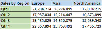
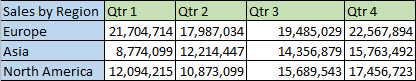
The Transpose feature will rearrange the table such that the Quarters are showing in the column headings and the Sales Regions can be seen on the left, like this:
Note: If your data is in an Excel table, the Transpose feature won’t be available. You can convert the table to a range first, or you can use the TRANSPOSE function to rotate the rows and columns.
Here’s how to do it:
Select the range of data you want to rearrange, including any row or column labels, and press Ctrl+C.
Note: Ensure that you copy the data to do this, since using the Cut command or Ctrl+X won’t work.
Choose a new location in the worksheet where you want to paste the transposed table, ensuring that there is plenty of room to paste your data. The new table that you paste there will entirely overwrite any data / formatting that’s already there.
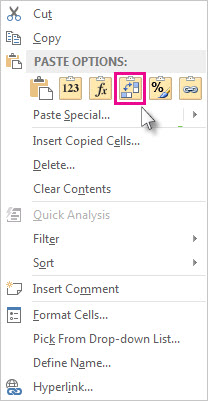
Right-click over the top-left cell of where you want to paste the transposed table, then choose Transpose  .
.
After rotating the data successfully, you can delete the original table and the data in the new table will remain intact.
Tips for transposing your data
If your data includes formulas, Excel automatically updates them to match the new placement. Verify these formulas use absolute references—if they don’t, you can switch between relative, absolute, and mixed references before you rotate the data.
If you want to rotate your data frequently to view it from different angles, consider creating a PivotTable so that you can quickly pivot your data by dragging fields from the Rows area to the Columns area (or vice versa) in the PivotTable Field List.
You can paste data as transposed data within your workbook. Transpose reorients the content of copied cells when pasting. Data in rows is pasted into columns and vice versa.
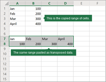
Here’s how you can transpose cell content:
Copy the cell range.
Select the empty cells where you want to paste the transposed data.
On the Home tab, click the Paste icon, and select Paste Transpose.
Need more help?
You can always ask an expert in the Excel Tech Community or get support in the Answers community.
Источник
How to Reverse a Column Order in Microsoft Excel

Reversing the order of a column would be easy if the column was already listed alphabetically or sequentially; you would just sort in the other direction. However, data may not be in alphabetical or numerical order, so applying the sort function directly to the data will rearrange the records, rather than simply reverse them. As an example, imagine a data list displaying days of the week — Monday through Friday. There is certainly an order to them, but sorting them will rearrange the days, instead of listing Friday through Monday. Although Excel offers no automated solution, you can number the entries and sort by that new column.
Right-click the column letter of the column you want to sort, and select «Insert» to create a new column.
Enter «1» in the first cell of the new column and «2» in the second cell.
Drag your mouse over those two number cells to select them, and point to the lower-right corner of the selection until your mouse pointer turns into a «+.» Click and drag your mouse to the cell that corresponds to the last data record of the original column. When you release your mouse button, Excel automatically fills the other cells with a sequential series of numbers.
Drag your mouse across the data and number cells to select them.
Click the «Data» tab and click «Sort» from the Sort & Filter section.
Select the number column from the «Sort by» drop-down menu and select «Largest to Smallest» from the «Order» drop-down menu.
Источник
How to flip data in Excel: reverse columns vertically and rows horizontally
 by Svetlana Cheusheva, updated on March 20, 2023
The tutorial shows a few quick ways to flip tables in Excel vertically and horizontally preserving the original formatting and formulas.
Flipping data in Excel sounds like a trivial one-click task, but surprisingly there is no such built-in option. In situations when you need to reverse the data order in a column arranged alphabetically or from smallest to largest, you can obviously use the Excel Sort feature. But how do you flip a column with unsorted data? Or, how do you reverse the order of data in a table horizontally in rows? You will get all answers in a moment.
Flip data in Excel vertically
With just a little creativity, you can work out a handful of different ways to flip a column in Excel: by using inbuilt features, formulas, VBA or special tools. The detailed steps on each method follow below.
How to flip a column in Excel
The reverse the order of data in a column vertically, perform these steps:
- Add a helper column next to the column you want to flip and populate that column with a sequence of numbers, starting with 1. This tip shows how to have it done automatically.
- Sort the column of numbers in descending order. For this, select any cell in the helper column, go to the Data tab >Sort & Filter group, and click the Sort Largest to Smallest button (ZA).
As shown in the screenshot below, this will sort not only the numbers in column B, but also the original items in column A, reversing the order of rows:

Now you can safely delete the helper column since you do not need it any longer.
Tip: How to quickly fill a column with serial numbers
The fastest way to populate a column with a sequence of numbers is by using the Excel AutoFill feature:
- Type 1 into the first cell and 2 into the second cell (cells B2 and B3 in the screenshot below).
- Select the cells where you’ve just entered the numbers and double-click the lower right corner of the selection.

That’s it! Excel will autofill the column with serial numbers up to the last cell with data in the adjacent column.
How to flip a table in Excel
The above method also works for reversing the data order in multiple columns:
Sometimes (most often when you select the whole column of numbers prior to sorting) Excel might display the Sort Warning dialog. In this case, check the Expand the selection option, and then click the Sort button.

Tip. If you’d like to switch rows and columns, use the Excel TRANSPOSE function or other ways to transpose data in Excel.
How to flip columns in Excel using a formula
Another way to flip a column upside down is by using this generic formula:
For our sample data set, the formula goes as follows:
…and reverses column A impeccably:

How this formula works
At the heart of the formula is the INDEX(array, row_num, [column_num]) function, which returns the value of an element in array based on the row and/or column numbers you specify.
In the array, you feed the entire list you want to flip (A2:A7 in this example).
The row number is worked out by the ROWS function. In its simplest form, ROWS(array) returns the number of rows in array. In our formula, it’s the clever use of the relative and absolute references that does the «flip column» trick:
- For the first cell (B2), ROWS(A2:$A$7) returns 6, so INDEX gets the last item in the list (the 6 th item).
- In the second cell (B3), the relative reference A2 changes to A3, consequently ROWS(A3:$A$7) returns 5, forcing INDEX to fetch the second to last item.
In other words, ROWS creates a kind of decrementing counter for INDEX so that it moves from the last item toward the first item.
Tip: How to replace formulas with values
Now that you have two columns of data, you may want to replace formulas with calculated values, and then delete an extra column. For this, copy the formula cells, select the cells where you’d like to paste the values, and press Shift+F10 then V , which is the fastest way to apply Excel’s Paste Special > Values option.

How to flip columns in Excel with VBA
If you have some experience with VBA, you can use the following macro to reverse the data order vertically in one or several columns:
How to use the Flip Columns macro
- Open the Microsoft Visual Basic for Applications window ( Alt + F11 ).
- Click Insert >Module, and paste the above code in the Code window.
- Run the macro ( F5 ).
- The Flip Columns dialog pops up prompting you to select a range to flip:
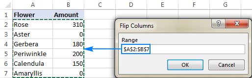
You select one or more columns using the mouse, not including the column headers, click OK and get the result in a moment.
To save the macro, be sure to save your file as an Excel macro-enabled workbook.
How to flip data in Excel preserving formatting and formulas
With the above methods, you can easily reverse the data order in a column or table. But what if you not only wish to flip values, but cell formats too? Additionally, what if some data in your table is formula-driven, and you want to prevent formulas from being broken when flipping columns? In this case, you can use the Flip feature included with our Ultimate Suite for Excel.
Supposing you have a nicely formatted table like shown below, where some columns contain values and some columns have formulas:

You are looking to flip the columns in your table keeping both formatting (grey shading for rows with zero qty.) and correctly calculated formulas. This can be done in two quick steps:
- With any cell in your table selected, go to the Ablebits Data tab >Transform group, and click Flip >Vertical Flip.

- In the Select your range box, check the range reference and make sure the header row is not included.
- Select the Adjust cell references option and check the Preserve formatting box.
- Optionally, choose to Create a back up copy (selected by default).
- Click the Flip button.

Done! The order of data in the table is reversed, the formatting is kept, and cell references in the formulas are appropriately adjusted:

Flip data in Excel horizontally
So far in this tutorial, we have flipped columns upside down. Now, let’s look at how to reverse data order horizontally, i.e. flip a table from left to right.
How to flip rows in Excel
As there is no option to sort rows in Excel, you’ll need to first change rows to columns, then sort columns, and then transpose your table back. Here are the detailed steps:
- Use the Paste Special > Transpose feature to convert columns to rows. As the result, your table will undergo this transformation:
![]()
Add a helper column with numbers as in the very first example, and then sort by the helper column. Your intermediate result will look something like this:
![]()
Use Paste Special > Transpose one more time to rotate your table back:
![]()
Note. If your source data contains formulas, they may be broken during the transpose operation. In this case, you will have to restore the formulas manually. Or you can use the Flip tool included in our Ultimate Suite and it will adjust all the references for you automatically.
Reverse data order horizontally with VBA
Here is a simple macro that can quickly flip data in your Excel table horizontally:
To add the macro to your Excel workbook, please follow these steps. As soon as you run the macro, the following dialog window will show up, asking you to select a range:
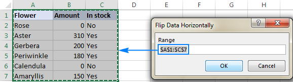
You select the entire table, including the header row, and click OK. In a moment, the data order in rows in reversed:
Flip data in rows with Ultimate Suite for Excel
Similarly to flipping columns, you can use our Ultimate Suite for Excel to reverse the order data in rows. Just select a range of cells you want to flip, go to the Ablebits Data tab > Transform group, and click Flip > Horizontal Flip.

In the Horizontal Flip dialog window, choose the options appropriate for your data set. In this example, we are working with values, so we choose Paste values only and Preserve Formatting:

Click the Flip button, and your table will be reversed from left to right in the blink of an eye.
This is how you flip data in Excel. I thank you for reading and hope to see you on our blog next week!
Источник
На чтение 4 мин Просмотров 1к. Опубликовано 27.04.2022
Бывают ситуации, когда вам нужно «перевернуть» вашу табличку. То есть сделать так, чтобы данные, которые находятся вверху — были внизу.
И да, это удивительно, но в программе нет специальной функции для этого.
Конечно же, мы можем сделать это сразу несколькими методами. Но именно своей функции для такой задачи в Excel нет.
Итак, начнём!
Содержание
- С помощью функции «Сортировка»
- По вертикали
- По горизонтали
- C помощью СОРТПО и ИНДЕКС
- С помощью СОРТПО
- С помощью ИНДЕКС
- С помощью Visual Basic
С помощью функции «Сортировка»
Это, наверное, самый быстрый и удобный метод.
По вертикали
Допустим, нам нужно отсортировать данные в обратном порядке, для следующей таблички:

Пошаговая инструкция:
- Создайте столбик для расчетов (мы назовем его «Helper»);
- Выделите табличку и щелкните на «Данные»;

- Далее — «Сортировка»;
- В первом параметре сортировки выберите наш столбик для расчетов;
- А в третьем — «По убыванию»;
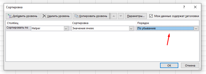
- Подтвердите.
Готово! Вот результат:
После сортировки можно удалить столбик для расчетов.
Мы рассмотрели табличку, в которой есть только один столбик с данными(не считая имен). Но его можно использовать независимо от того, сколько у вас столбиков с данными.
По горизонтали
Практически тоже самое с табличками по горизонтали.
Итак, давайте рассмотрим такой пример.
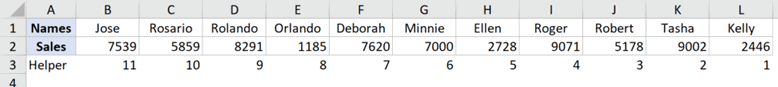
Допустим, у нас есть такая табличка:

Пошаговая инструкция:
- Создаем столбик для расчетов, только теперь это не столбик, а строка. Так как табличка у нас горизонтальная;

- Открываем «Сортировка»;
- Жмем «Параметры…»;
- И выберите «Столбцы диапазона»;
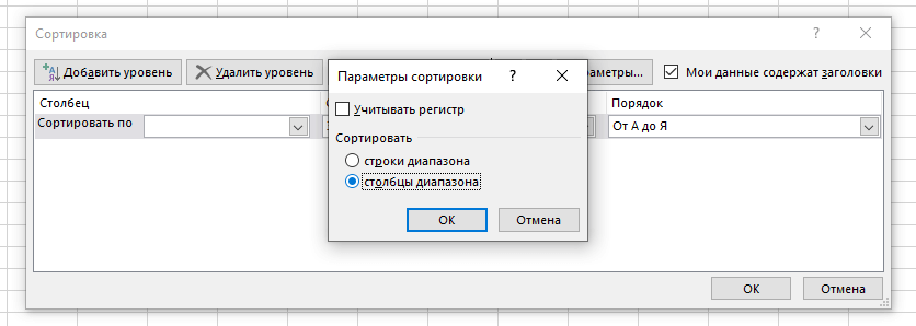
- Подтвердите;
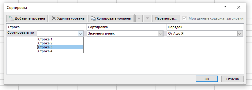
- В первом параметре выберите ту строку, которая является строкой для расчетов.
- В третьем параметре — «По убыванию»;
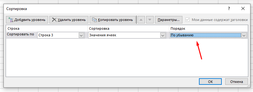
- Подтвердите.
Готово! Вот результат:
После сортировки можете смело удалять строку для расчетов.
C помощью СОРТПО и ИНДЕКС
Функция ИНДЕКС доступна для всех, а вот функция СОРТПО доступна только по платной подписке Office 365.
С помощью СОРТПО
Допустим, у нас есть такая табличка:
Создадим еще два столбика, с теме же заголовками. Там будет наша обработанная табличка.
Формула функции примет такой вид:
=СОРТПО($A$2:$B$12;СТРОКА(A2:A12);-1)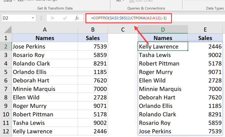
Сортировка происходит по данным, полученным из функции СТРОКА.
Она создает массив с порядковыми номерами строк.
А последний аргумент в функции (“-1”) говорит Excel о том, что нам нужен порядок «По убыванию».
Вот, собственно, и все!
С помощью ИНДЕКС
Мало кто пользуется Microsoft 365 и платит за подписку, но не переживайте, если вы из таких людей, то для вас есть выход!
Допустим, у нас та же табличка:
Формула примет такой вид:
=ИНДЕКС($A$2:$A$12;СТРОКА(A2:$A$12))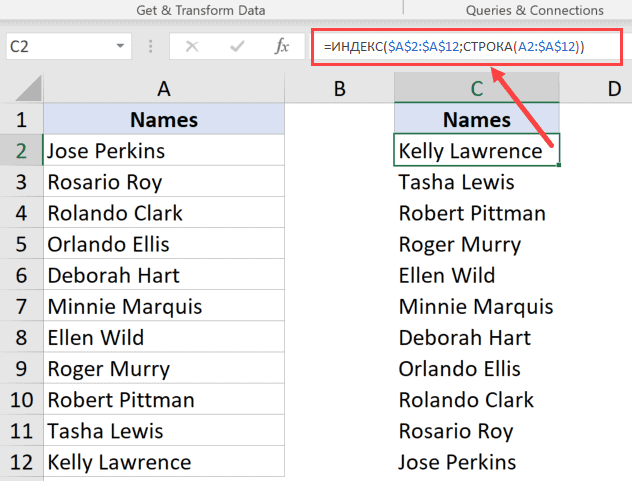
Что мы сделали?
Функция СТРОКА, в результате выполнения, отдает нам кол-во строчек в диапазоне ячеек.
И этот результат будет становиться меньше и меньше.
А ИНДЕКС, по номеру строки, отдает нам значение этой строки. Таким образом мы получаем порядок «По убыванию».
Так же, как и в предыдущих методах, функцию можно использовать в табличке с несколькими столбиками данных. Но, в аргументе, вам нужно будет указать, откуда функции брать данные для обработки.
Допустим, у вас есть такая табличка:
Формула примет такой вид:
=ИНДЕКС($A$2:$B$12;СТРОКА(A2:$A$12);СТОЛБЕЦ($A$2:A2))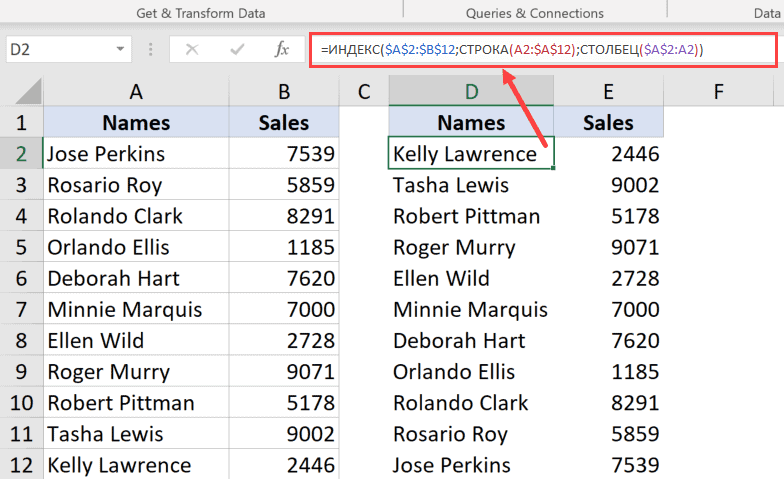
Все также, только мы дополнительно указали столбик, откуда функция ИНДЕКС должна брать данные и помещать в новые ячейки.
Если вы решили отсортировать данные — помните, что отменить сортировку у вас не получится. Если исходная сортировка для вас важна, то сделайте копию оригинальной таблички.
С помощью Visual Basic
И, как обычно, рассмотрим метод с Visual Basic.
Это решение отлично подойдет для тех, кто использует такую сортировку очень часто.
Вот нужный нам код Visual Basic:
Sub FlipVerically()

Dim TopRow As Variant
Dim LastRow As Variant
Dim StartNum As Integer
Dim EndNum As Integer

Application.ScreenUpdating = False

StartNum = 1
EndNum = Selection.Rows.Count

Do While StartNum < EndNum
TopRow = Selection.Rows(StartNum)
LastRow = Selection.Rows(EndNum)
Selection.Rows(EndNum) = TopRow
Selection.Rows(StartNum) = LastRow
StartNum = StartNum + 1
EndNum = EndNum - 1
Loop

Application.ScreenUpdating = True
End Sub
Очень важно, если вы хотите использовать функцию, которую мы создали с помощью этого кода — не выделяйте заголовки таблички.
Куда нужно поместить код?
Пошаговая инструкция:
- ALT + F11;
- Правой кнопкой мышки на любой лист -> «Insert» -> «Module»;
- В открывшееся окошко вставьте наш код и закройте Visual Basic;
А дальше, чтобы использовать функцию — выделите табличку и нажмите «Run Macro» (или F5).
В этой статье, я рассказал вам о том, как можно отсортировать данные в обратном порядке. Мы рассмотрели как сделать это с помощью встроенной функции “Сортировка”, с помощью СОРТПО и ИНДЕКС, а также Visual Basic.
Надеюсь, эта статья оказалась полезна для вас!
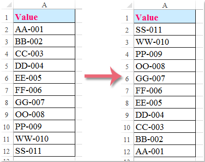
Sometimes, you may want to flip a column of data order vertically in Excel as the left screenshot shown. It seems quite hard to reverse the data order manually, especially for a lot of data in the column. This article will guide you to flip or reverse a column data order vertically quickly.
Flip a column of data order in Excel with Sort command
Flip a column of data order in Excel with VBA
Several clicks to flip a column of data order with Kutools for Excel
Flip a column of data order in Excel with Sort command
Using Sort command can help you flip a column of data in Excel with following steps:
1. Insert a series of sequence numbers besides the column. In this case, in insert 1, 2, 3…, 7 in Column B, then select B2:B12, see screenshot:

2. Click the Data > Sort Z to A, see screenshot:

3. In the Sort Warning dialog box, check the Expand the selection option, and click the Sort button.

4. Then you will see the number order of Column A is flipped. And you can delete or hide the Column B according to your needs. See the following screenshot:

This method is also applied to reversing multiple columns of data order.
Flip a column of data order in Excel with VBA
If you know how to use a VBA code in Excel, you may flip / reverse data order vertically as follows:
1. Hold down the Alt + F11 keys in Excel, and it opens the Microsoft Visual Basic for Applications window.
2. Click Insert > Module, and paste the following macro in the Module Window.
VBA: Flip / reverse a range data order vertically in Excel.
Sub FlipColumns()
'Updateby20131126
Dim Rng As Range
Dim WorkRng As Range
Dim Arr As Variant
Dim i As Integer, j As Integer, k As Integer
On Error Resume Next
xTitleId = "KutoolsforExcel"
Set WorkRng = Application.Selection
Set WorkRng = Application.InputBox("Range", xTitleId, WorkRng.Address, Type:=8)
Arr = WorkRng.Formula
For j = 1 To UBound(Arr, 2)
    k = UBound(Arr, 1)
    For i = 1 To UBound(Arr, 1) / 2
        xTemp = Arr(i, j)
        Arr(i, j) = Arr(k, j)
        Arr(k, j) = xTemp
        k = k - 1
    Next
Next
WorkRng.Formula = Arr
End Sub
3. Press the F5 key to run this macro, a dialog is popped up for you to select a range to flip vertically, see screenshot:

4. Click OK in the dialog, the range is flipped vertically, see screenshot:
Several clicks to flip a column of data order with Kutools for Excel
If you have Kutools for Excel installed, you can reverse the numbers order of columns with Flip Vertical Range tool quickly.
1. Select the column of date you will flip vertically, then click Kutools > Range > Flip Vertical Range > All / Only flip values. See screenshot:

Note: If you want to flip vaues along with cell formatting, plesae select the All option. For only flipping values, please select the Only flip values option.
Then the selected data in the column has been flipped vertically. See screenshot:
Tip: If you also need to flip data horizontally in Excel. Please try the Flip Horizontal Range utility of Kutools for Excel. You just need to select two ranges firstly, and then apply the utility to acheive it as below screenshot shown.

Then the selected ranges are flipped horizontally immediately.

If you want to have a free trial (30-day) of this utility, please click to download it, and then go to apply the operation according above steps.
Demo: flip / reverse a column of data order vertically
Related article:
How to flip / reverse a row of data order in Excel quickly?
The Best Office Productivity Tools
Kutools for Excel Solves Most of Your Problems, and Increases Your Productivity by 80%
- Reuse: Quickly insert complex formulas, charts and anything that you have used before; Encrypt Cells with password; Create Mailing List and send emails…
- Super Formula Bar (easily edit multiple lines of text and formula); Reading Layout (easily read and edit large numbers of cells); Paste to Filtered Range…
- Merge Cells/Rows/Columns without losing Data; Split Cells Content; Combine Duplicate Rows/Columns… Prevent Duplicate Cells; Compare Ranges…
- Select Duplicate or Unique Rows; Select Blank Rows (all cells are empty); Super Find and Fuzzy Find in Many Workbooks; Random Select…
- Exact Copy Multiple Cells without changing formula reference; Auto Create References to Multiple Sheets; Insert Bullets, Check Boxes and more…
- Extract Text, Add Text, Remove by Position, Remove Space; Create and Print Paging Subtotals; Convert Between Cells Content and Comments…
- Super Filter (save and apply filter schemes to other sheets); Advanced Sort by month/week/day, frequency and more; Special Filter by bold, italic…
- Combine Workbooks and WorkSheets; Merge Tables based on key columns; Split Data into Multiple Sheets; Batch Convert xls, xlsx and PDF…
- More than 300 powerful features. Supports Office / Excel 2007-2021 and 365. Supports all languages. Easy deploying in your enterprise or organization. Full features 30-day free trial. 60-day money back guarantee.
")
Office Tab Brings Tabbed interface to Office, and Make Your Work Much Easier
- Enable tabbed editing and reading in Word, Excel, PowerPoint, Publisher, Access, Visio and Project.
- Open and create multiple documents in new tabs of the same window, rather than in new windows.
- Increases your productivity by 50%, and reduces hundreds of mouse clicks for you every day!
")
When trying to flip data, be it a column, row, or table in Excel, you would probably find that there’s no built-in option to do this.
If your data is arranged in alphabetical order, it would of course be easier to just use the Sort feature to reverse the order.
However, for an unsorted list, reversing the order is not that simple.
In this tutorial we will show you different ways to flip data in different situations:
- When you want to flip a column
- When you want to flip a row
- When you want to flip a table
- When you want to switch rows and columns
Flipping a column may seem like a one-click task, but if it consists of an unsorted list of items, flipping a column is not just about re-sorting the items.
Let us look at three ways to flip a column in Excel:
- Using a Helper Column
- Using a Formula
- Using VBA
To demonstrate the three methods we will use the following list of items:

Using each method, we will show you how to flip the above list of items, so that they are displayed in the reverse order.
Using a Helper Column to Flip a Column in Excel
The first method requires the use of an additional “Helper” column which will contain numbers 1,2,3… in ascending order.
This column will work as a sort of ‘index’ column, with each number serving as an index for the corresponding list item.
Once this helper column is ready all that we need to do is select both columns and sort the helper column in descending order!
Here are the steps to make this happen:
- If the column next to the one that you want to flip is not empty, then add a blank new column next to it (by right clicking on the column heading and selecting ‘Insert’).
- Fill this empty column (column B in our case) with numbers. Start by typing 1 in the first cell, 2 in the second cell and then using the fill handle (or flash fill) to create a series of numbers that end at the row corresponding to the last item of the list.

- Select both columns (columns A and B in our case) and navigate to Data->Sort from the main menu.

- This will open the Sort dialog box.
- Click on the dropdown arrow next to ‘Sort by’ and select the column that you just added and filled with numbers (the ‘Helper’ column in our case).

- Under ‘Order’, select ‘Largest to Smallest’. This will make sure that the selected columns are sorted by the Helper column in descending order.

- Click OK.
You should now get both columns reversed (or flipped).

Once your intended column is flipped, you can go ahead and delete the Helper column (column B).

You can use this same technique to flip a whole table.
Using a Formula to Flip a Column in Excel
If you want to get the job done in fewer steps, you could use formula instead.
The formula to flip a column in Excel involves the use of the INDEX and ROWS functions.
Let us first individually look at what each of these functions does.
The INDEX Function
The INDEX function is used to find the value at a given index of a given range. The syntax for the INDEX function is:
INDEX(array, row_num, [column_num])
Here,
- array is an array or range of cells from which we want to select a value to be returned
- row_num is an integer that specifies the index of the value (within array) that we want returned by the function
- column_num is an integer that specifies the column number (within array) from which we want to return a value. This parameter is optional.
The INDEX function simply selects the value from within the array that falls in the row and column corresponding to row_num and column_num.
If we omit the column_num parameter, then the INDEX function returns the value in the array that is at index row_num.
For example, the following formula, when applied to our sample data list will return the value at the 5th index of the list (or the 5th item):
=INDEX(A2:A7, 5)

The ROWS Function
The ROWS function simply returns the number of rows in a given range. The syntax for the ROWS function is:
ROWS(array)
Here, the array is an array or range of cells for which we want to find the number of rows.
For example, if we apply the ROWS formula to our sample data list, it will return the number of rows in this list:
=ROWS(A2:A7)

Using INDEX and ROWS Functions to Flip a Column in Excel
To flip the column in our sample data set, we need to follow the steps shown below:
- If the column next to the one that you want to flip is not empty, then add a blank new column next to it (by right clicking on the column heading and selecting ‘Insert’).
- Now type the formula: =INDEX($A$2:$A$7,ROWS(A2:$A$7)).
- Copy the formula down to the rest of the cells in the column using the fill handle.
You should now get the same list as your original column, but in reverse order.

This method helps you flip the column, while still retaining the original column as it is.
So it’s quite useful when you want to make sure the original list remains untouched.
Once you get the flipped list, you can copy the list and Paste it as the value in place of the original column (column A in our case) if you need to.

Explanation of the Formula
The ROWS function performs the main task of working out the indexes.
Notice we specified the starting cell reference for the ROWS function as a relative reference (A2), while we specified the ending cell reference as an absolute reference ($A$7).
This makes sure that each time the formula is copied, the ending reference stays the same while the starting reference keeps changing.
This means that in the first cell, the formula is ROWS(A2:$A$7), which returns the value 6 (since there are only 6 rows in the range).
This makes the INDEX function return the item at index 6 of our list, which is the last item.
In the second cell, the formula is ROWS(A3:$A$7), which returns the value 5 (since there are only 5 rows in the range).
This makes the INDEX function return the item at index 5 of our list, which is the second to last item.
This goes on till the last cell, the formula is ROWS(A7:$A$7), which returns the value 1. This makes the INDEX function return the first item in the list.
In other words, the ROWS function basically acts like our Helper column (from our first method).
It creates a decrementing counter for the INDEX function, which keeps moving from the first to the last item in the list.
Also read: How to Rearrange Rows In Excel
Using VBA to Flip a Column in Excel
The third way to flip a column in Excel is to use VBA code. Here is the code that we will be using to accomplish this:
'Code developed by Steve Scott from SpreadsheetPlanet.com
Sub FlipColumn()
Dim rng As Range
Dim result As Range
Dim start_index As Integer
Dim end_index As Integer
Set rng = Selection
start_index = 1
end_index = Selection.Rows.Count
Do While start_index < end_index
val1 = Selection.Rows(start_index)
val2 = Selection.Rows(end_index)
Selection.Rows(end_index) = val1
Selection.Rows(start_index) = val2
start_index = start_index + 1
end_index = end_index – 1
Loop
End Sub
Copy this code into your Developer window.
To run this code, simply select the column that you want to flip and then run this macro by following the steps shown below:
- From the Developer menu, select Macros.

- This opens the Macro dialog box. Select the Macro named ‘FlipColumn’ from the list under ‘Macro Name’.

- Click Run.
You should now find your selected column flipped.

Explanation of the Script
The above script takes the selected column and first counts the number of cells in it. The code stores the number of cells in a variable called end_index.
end_index = Selection.Rows.Count
In the same way, it stores the starting index of the list (which is 1) in a variable called start_index.
start_index = 1
Next, the code takes the first and last cells of the list, and interchanges them. It does this by using the start_index value to locate the first cell in the list and the end_index value to locate the last cell in the list.
val1 = Selection.Rows(start_index)
val2 = Selection.Rows(end_index)
The code repeatedly performs this action, each time increasing the start_index and decreasing the end_index values, until both become equal.
By doing this, we are shortening the list under consideration at each loop iteration until there are no more items left.
Do While start_index < end_index
val1 = Selection.Rows(start_index)
val2 = Selection.Rows(end_index)
    Selection.Rows(end_index) = val1
    Selection.Rows(start_index) = val2
start_index = start_index + 1
end_index = end_index - 1
Loop
This is how it gives us a column with all its data reversed.
Also read: Transpose in Excel (Keyboard Shortcut)
How to Flip a Table in Excel
If, instead of a single column, you want to flip a whole table of columns, then all you need to do is extend the above techniques to a set of columns.
For example, let’s say you have the following table consisting of two columns that you want to flip.

To flip this table, you can use the first method to flip a column (using the Helper column), after you’ve filled the helper column with number indexes, simply select all the columns of your table along with the helper column.

When you sort the selected table by the Helper column, Excel might display a Sort Warning dialog as shown below:

Simply check the ‘Expand the selection’ option and then click the Sort button. Your entire table should now get flipped.

After this, you can go ahead and delete the Helper column.

How to Flip / Switch Columns and Rows
You might have come across this tutorial looking for a way to flip or in fact switch rows and columns.
In other words, you might want to convert your rows to columns and columns to rows. In that case, you will need to use a special Excel feature that does just that.
Let us see how to apply this feature to the following table and flip its rows and columns:

Excel’s Transpose feature lets you transpose an array, table or range of cells. To apply this feature to your data, follow the steps outlined below:
- Make sure you have a blank area of cells where you can place your flipped table.
- Select the table that you want to flip rows and columns for.
- Copy the table by using the keyboard shortcut CTRL+C or right-clicking on your selection and selecting Copy.
- Select the top-left corner cell of your blank area of cells.
- Right click on this cell and select Paste Special from the context menu that appears.

- This opens the Paste Special dialog box. Check the box next to ‘Transpose’.

- Click OK.
You should now get a flipped version of your original table, where the rows and columns are switched.

Also read: How to Convert Columns to Rows in Excel?
How to Flip Rows in Excel
Now let’s look at a case where we want to flip a row in Excel.
Say you want to flip the row shown below:

Flipping a row in Excel is different from flipping a column. This is because, unlike columns, Excel does not provide any feature to sort rows.
So, you will need to perform a few additional steps.
To flip a row in Excel, you need to use a combination of tricks that you learned in this tutorial.
Since Excel does not support the sorting of rows, you will need to first transpose the row into a column (using the Transpose feature), and then flip it like any column.
Once done you can transpose the flipped column back into a row.
So the steps to flip a row are as follows:
- Select the row that you want to flip.
- Transpose this row into a column by copying it (pressing CTRL+C), right-clicking and selecting Paste Special from the context menu. Next check the box next to ‘Transpose’.
- Your row should now have turned into a column.

- Next, insert a Helper column containing numbers 1,2, … in sequence.

- Select both columns and navigate to Data->Sort.
- Select your helper column name from the ‘Sort by’ drop down list.
- Select ‘Largest to Smallest’ from the ‘Order’ drop down list.
- Click OK.
- Your column data should now be flipped.

- Finally, transpose the column back to a row by repeating step 2.

- Delete the Helper row.
You should now get your row back, but with its data flipped.
In this tutorial, we showed you different ways to flip data in Excel.
It might have come across as lengthy, but we tried to include different kinds of situations that you might come across and how to flip your data in each situation.
You can select the method which best serves your requirements.
We hope the tutorial was helpful for you.
Other articles you may also like:
- How to Sort by Date in Excel
- How to Move Row to Another Sheet Based On Cell Value in Excel?
- How to Unmerge All Cells in Excel? 3 Simple Ways
- How to Compare Two Columns in Excel (using VLOOKUP & IF)
- How to Swap Columns in Excel?
- How to Split One Column into Multiple Columns in Excel
- How to Make Positive Numbers Negative in Excel
- How to Combine Two Columns in Excel (with Space/Comma)