Returns in excel cell - Word и Excel - помощь в работе с программами

Often when you’re entering data into a Microsoft Excel spreadsheet, you want certain cells to span multiple lines, either for addresses, multiline pieces of information or just for readability. But if you press enter in an Excel cell, it will move you to the next cell down rather than inserting a line break.

Tip

To create a new line in an Excel cell, hold down the alt key on your keyboard while hitting enter.

Insert Line Break in Excel

To move to a new line in an Excel cell, simply type text in the cell as normal and then press enter while holding down the alt key. If you need to move to a specific place in the cell to enter a new line, double-click the cell with your mouse and then click the specific place you want to enter the line break. Then hit enter while holding down alt.

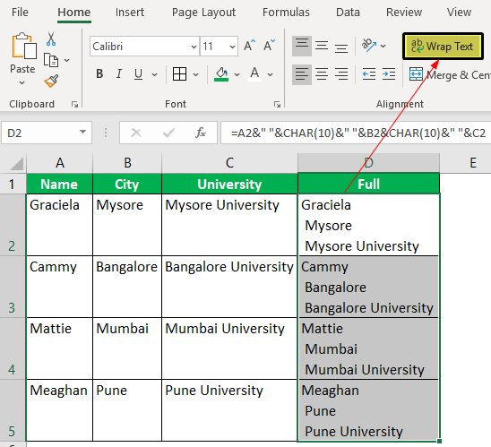
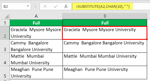
If you need to have a formula output break onto a new line to go into an Excel cell, you can do this as well. To do so, include in the formula the bit «& CHAR(10) &» wherever you want the formula’s output to break lines if you’re using Windows. That tells Excel to insert the character numbered as 10 in the computer’s character set, which on Windows is a line break character. If you’re using a MacOS computer, use the number 13 rather than 10 for the same effect.

Wrapping Text in Excel

In some cases, you may have too much text in an Excel cell to fit on one line. In this case, you may want the text to wrap onto another line automatically. To enable this feature, select the cells that you want to automatically wrap. Then, on the «Home» tab in the ribbon menu, click «Alignment,» then the «Wrap Text» button.

If the cell’s height is not fixed, the text will automatically wrap from line to line and all the text should be visible. If you need to adjust the cell’s height, you can physically drag the edges of the cell using your mouse or using the Cell Size menu.

To do that, select the cells you’re interested in and click the «Home» tab.» Click the «Cells» group, then click «Format» and under «Cell Size,» click «AutoFit Row Height» to make the cell automatically adjust its height.

If you’d prefer to have a fixed height that might not contain all the text, click «Row Height» instead of «AutoFit Row Height» and enter your desired height.

Источник

What is Carriage Return in Excel Cell?

Carriage return in Excel cell is the activity used to push some of the cell’s content to the new line within the same cell. For example, when combining multiple cell data into one cell, we may want to push some content to the next line to make it look neat and organized.

For example, suppose you have a dataset with different subjects in different columns, and we need to combine those in a single cell in Excel. Here, the carriage return in the Excel method may help you add a line break within a single cell without using multiple lines of cells. In addition, it can also push some text to the next line in the same cell and allows data to have a competent look.

What is Carriage Return in Excel Cell?
- How to Insert a Carriage Return in Excel?
- Insert Excel Carriage Return by using Formula
- How to Remove Carriage Return Character from Excel Cell?
- Things to Remember
- Recommended Articles

How to Insert a Carriage Return in Excel?

You can download this Carriage Return Excel Template here – Carriage Return Excel Template

So, we can say, “a line breaker or newline inserted within the same cell to push some of the contents of the next line.”

We must follow the steps to insert carriage return in Excel.

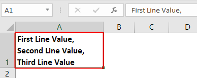
For example, let us look at the below data set.

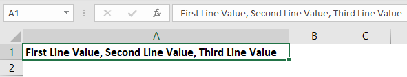
We have three sentences in cell A1, separating each by a comma (,). So, in this case, we need to push the second line to the next line and the third line to the next line, like the one below.
As you can see above, it has reduced the row’s width and increased its height by placing a carriage return character.
Ok, let’s get back to this and see how we can insert a carriage return. First, our data looks like this in a cell.
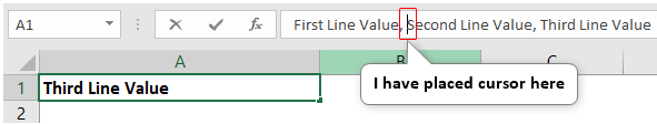
We will place a cursor before the content, which we must push to the next line.
We will press the excel shortcut key ALT + ENTER to insert the carriage return character in the Excel cell.

Pressing the “ALT + ENTER” key pushes the content in front of the selected data to the new line by inserting a carriage return.
Now again, place a cursor in front of the third-line data.
Next again, we will press the shortcut key ALT + ENTER.

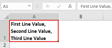
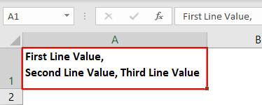
It has inserted the carriage return character to push the data to the new line within the same cell.

Insert Excel Carriage Return by using Formula

In the case of concatenating values of different cells, we may need to push a couple of data to the next line.

For example, let us look at the below data

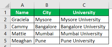
We need to combine these cell values from the above data. But we also need each cell value to be in a new line like the one below.

Since we are dealing with more than one cell, it is a tough task to keep pressing the shortcut key all the time. So instead, we can use the character function “CHAR” to insert a carriage return.

Apply the below formula as shown below.

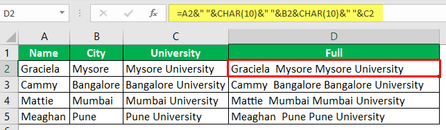
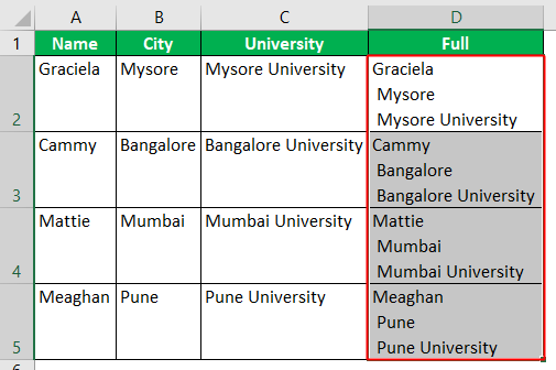
After applying the formula, we could see the flat row. But, we need to make one small adjustment, i.e., to wrap the formula used cells.

In this example, we have used the “CHAR(10)” function, which inserts the “carriage return” character wherever we have applied it.

How to Remove Carriage Return Character from Excel Cell?

If inserting the carriage return is the one skill, removing those carriage return characters is another set of skills we need to learn.

Assume we have got the below data from the web.

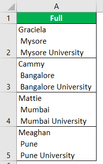
We can remove the carriage return character from an Excel cell using several methods. The first method is by using the replace method.

Select the data range and press the “Ctrl + H” shortcut key.

We need first to find the value we are replacing. In this case, we see the “carriage return” character. To insert this character, we need to press “Ctrl + J.”

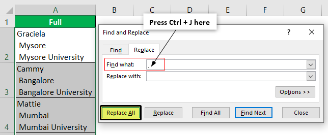
We need to remove the carriage return character so leave the “Replace with” part of this “Find and Replace” method.

Now, we will press the button “Replace All,” and it will remove all carriage return characters.

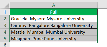
Another way of removing the carriage return character is by using a formula. Below is the formula to remove the carriage return character from the Excel cell.

Things to Remember

Carriage Return is adding a new line within the cellTo insert a new line in excel cell, a user can adopt any of the following three methods: Manually inserting a new line or using a shortcut key, Applying CHAR excel function, Using name manager with CHAR(10) function.read more.
CHAR (10) can insert a new line.
A combination of SUBSTITUTE in excelSubstitute function in excel is a very useful function which is used to replace or substitute a given text with another text in a given cell, this function is widely used when we send massive emails or messages in a bulk, instead of creating separate text for every user we use substitute function to replace the information.read more and CHAR functions can remove carriage return characters.

Method 1 — Cell Wrapping

Often, you need only set the cell to wrap text, and you can set the width of
the cell to whatever is desired. Choose FormatCells,
Alignment tab, and check Wrap text.

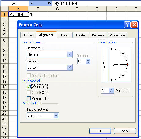
This is the result:

Method 2 — Insert a Return

This one’s a no-brainer. Just type the first line, hit Alt+Enter
and type the second line. The result is virtually the same as above, however, if
you copy and paste this to Word, for instance, you’ll end up with a line break.
Or if you export to CSV or other text format, you may get unexpected results.

Method 3 — Using a Formula

To use this, you must have wrap text selected. Here’s a sample
formula:

=a1&char(10)&a2

The results, again, are the same as above. However, if you
forget to wrap text on the cell, you’ll see this:

Источник

When using lookup formulas in Excel (such as VLOOKUP, XLOOKUP, or INDEX/MATCH), the intent is to find the matching value and get that value (or a corresponding value in the same row/column) as the result.

But in some cases, instead of getting the value, you may want the formula to return the cell address of the value.

This could be especially useful if you have a large data set and you want to find out the exact position of the lookup formula result.

There are some functions in Excel that designed to do exactly this.

In this tutorial, I will show you how you can find and return the cell address instead of the value in Excel using simple formulas.

Lookup And Return Cell Address Using the ADDRESS Function

The ADDRESS function in Excel is meant to exactly this.

It takes the row and the column number and gives you the cell address of that specific cell.

Below is the syntax of the ADDRESS function:

=ADDRESS(row_num, column_num, [abs_num], [a1], [sheet_text])

where:

row_num: Row number of the cell for which you want the cell address
column_num: Column number of the cell for which you want the address
[abs_num]: Optional argument where you can specify whether want the cell reference to be absolute, relative, or mixed.
[a1]: Optional argument where you can specify whether you want the reference in the R1C1 style or A1 style
[sheet_text]: Optional argument where you can specify whether you want to add the sheet name along with the cell address or not

Now, let’s take an example and see how this works.

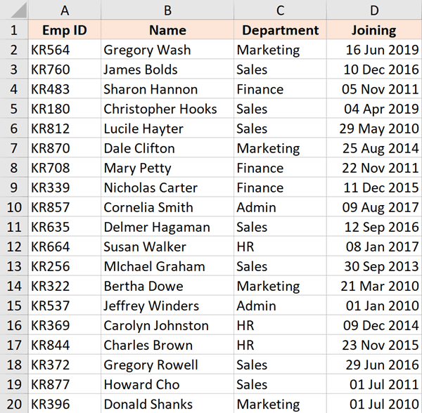
Suppose there is a dataset as shown below, where I have the Employee id, their name, and their department, and I want to quickly know the cell address that contains the department for employee id KR256.

Below is the formula that will do this:

=ADDRESS(MATCH("KR256",A1:A20,0),3)

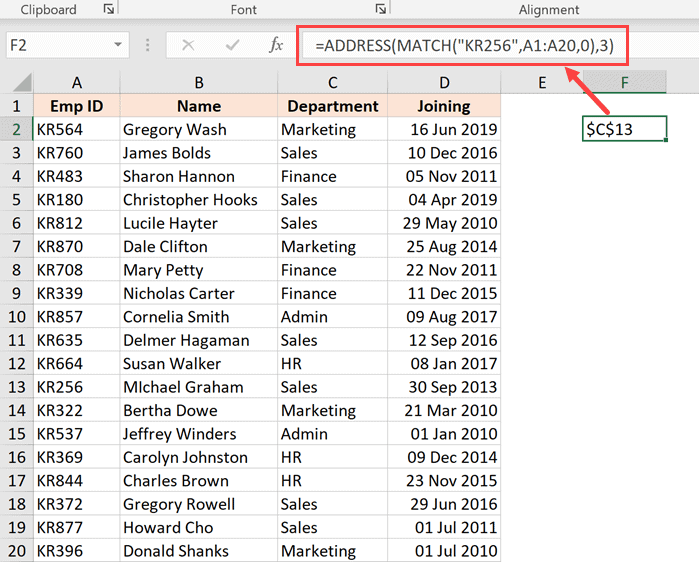
In the above formula, I have used the MATCH function to find out the row number that contains the given employee id.

And since the department is in column C, I have used 3 as the second argument.

This formula works great, but it has one drawback – it won’t work if you add the row above the dataset or a column to the left of the dataset.

This is because when I specify the second argument (the column number) as 3, it’s hard-coded and won’t change.

In case I add any column to the left of the dataset, the formula would count 3 columns from the beginning of the worksheet and not from the beginning of the dataset.

So, if you have a fixed dataset and need a simple formula, this will work fine.

But if you need this to be more fool-proof, use the one covered in the next section.

Lookup And Return Cell Address Using the CELL Function

While the ADDRESS function was made specifically to give you the cell reference of the specified row and column number, there is another function that also does this.

It’s called the CELL function (and it can give you a lot more information about the cell than the ADDRESS function).

Below is the syntax of the CELL function:

=CELL(info_type, [reference])

where:

info_type: the information about the cell you want. This could be the address, the column number, the file name, etc.
[reference]: Optional argument where you can specify the cell reference for which you need the cell information.

Now, let’s see an example where you can use this function to look up and get the cell reference.

Suppose you have a dataset as shown below, and you want to quickly know the cell address that contains the department for employee id KR256.

Below is the formula that will do this:

=CELL("address", INDEX($A$1:$D$20,MATCH("KR256",$A$1:$A$20,0),3))

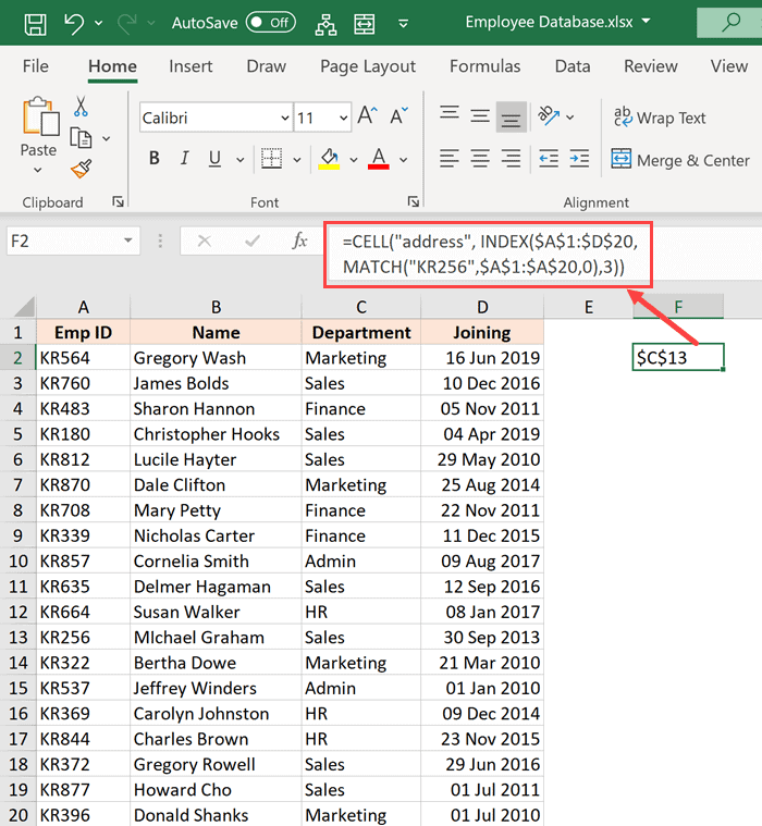
The above formula is quite straightforward.

I have used the INDEX formula as the second argument to get the department for the employee id KR256.

And then simply wrapped it within the CELL function and asked it to return the cell address of this value that I get from the INDEX formula.

Now here is the secret to why it works – the INDEX formula returns the lookup value when you give it all the necessary arguments. But at the same time, it would also return the cell reference of that resulting cell.

In our example, the INDEX formula returns “Sales” as the resulting value, but at the same time, you can also use it to give you the cell reference of that value instead of the value itself.

Normally, when you enter the INDEX formula in a cell, it returns the value because that is what it’s expected to do. But in scenarios where a cell reference is required, the INDEX formula will give you the cell reference.

In this example, that’s exactly what it does.

And the best part about using this formula is that it is not tied to the first cell in the worksheet. This means that you can select any data set (which could be anywhere in the worksheet), use the INDEX formula to do a regular look up and it would still give you the correct address.

And if you insert an additional row or column, the formula would adjust accordingly to give you the correct cell address.

So these are two simple formulas that you can use to look up and find and return the cell address instead of the value in Excel.

I hope you found this tutorial useful.

Other Excel tutorials you may also like:

Lookup and Return Values in an Entire Row/Column in Excel
Find the Last Occurrence of a Lookup Value a List in Excel
Lookup the Second, the Third, or the Nth Value in Excel
How to Reference Another Sheet or Workbook in Excel
Lookup and Return Values in an Entire Row/Column in Excel

Источник

Suppose I have a function attached to one of my Excel sheets:

Public Function foo(bar As Integer) as integer
    foo = 42
End Function

How can I get the results of foo returned to a cell on my sheet? I’ve tried "=foo(10)", but all it gives me is "#NAME?"

I’ve also tried =[filename]!foo(10) and [sheetname]!foo(10) with no change.

asked Feb 17, 2009 at 21:46

Try following the directions here to make sure you’re doing everything correctly, specifically about where to put it. ( Insert->Module )

I can confirm that opening up the VBA editor, using Insert->Module, and the following code:

Function TimesTwo(Value As Integer)
    TimesTwo = Value * 2
End Function

and on a sheet putting "=TimesTwo(100)" into a cell gives me 200.

BIBD

15k25 gold badges85 silver badges137 bronze badges

answered Feb 17, 2009 at 22:11

StephenStephen

4,0762 gold badges24 silver badges29 bronze badges

Put the function in a new, separate module (Insert->Module), then use =foo(10) within a cell formula to invoke it.

answered Feb 17, 2009 at 21:53

anormanorm

2,2471 gold badge19 silver badges38 bronze badges

Where did you put the «foo» function? I don’t know why, but whenever I’ve seen this, the solution is to record a dimple macro, and let Excel create a new module for that macro’s code. Then, put your «foo» function in that module. Your code works when I follow this procedure, but if I put it in the code module attached to «ThisWorkbook,» I get the #NAME result you report.

answered Feb 17, 2009 at 22:22

JeffKJeffK

3,0192 gold badges26 silver badges29 bronze badges

include the file name like this

=PERSONAL.XLS!foo(10)

answered Feb 17, 2009 at 21:50

chilltempchilltemp

8,8068 gold badges41 silver badges46 bronze badges

Источник

Author: Oscar Cronquist Article last updated on February 17, 2023

In this article, I will demonstrate four different formulas that allow you to lookup a value that is to be found in a given range and return the corresponding value on the same row. If you need to return multiple values because the ranges overlap then read this article: Return multiple values if in range.

What’s on this page

If value in range then return value — LOOKUP function
If value in range then return value — INDEX + SUMPRODUCT + ROW
If value in range then return value — VLOOKUP function
If value in range then return value — INDEX + MATCH

They all have their pros and cons and I will discuss those in great detail, they can be applied to not only numerical ranges but also text ranges and date ranges as well.

I have made a video that explains the LOOKUP function in context to this article, if you are interested.

There is a file for you to get, at the end of this article, which contains all the formula examples in a worksheet each.

You can use the techniques described in this article to calculate discount percentages based on price intervals or linear results based on the lookup value.

Check out the LOOKUP category to find more interesting articles.

The following table shows the differences between the formulas presented in this article.

Formula	Range sorted?	Array formula	Get value from any column?	Two range columns?
LOOKUP	Yes	No	Yes	No
INDEX + SUMPRODUCT + ROW	No	No	Yes	Yes
VLOOKUP	Yes	No	No	No
INDEX + MATCH	Yes	No	Yes	No

Some formulas require you to have the lookup range sorted to function properly, the INDEX+SUMPRODUCT+ROW alternative is the only way to go if you can’t sort the values.

The disadvantage with the INDEX+SUMPRODUCT+ROW formula is that you need start and end values, the other formulas use the start values also as end range values.

The VLOOKUP function can only search the leftmost column, you must rearrange your table to meet this condition if you are going to use the VLOOKUP function.

1. If value in range then return value — LOOKUP function

To better demonstrate the LOOKUP function I am going to answer the following question.

Hi,

What type of formula could be used if you weren’t using a date range and your data was not concatenated?

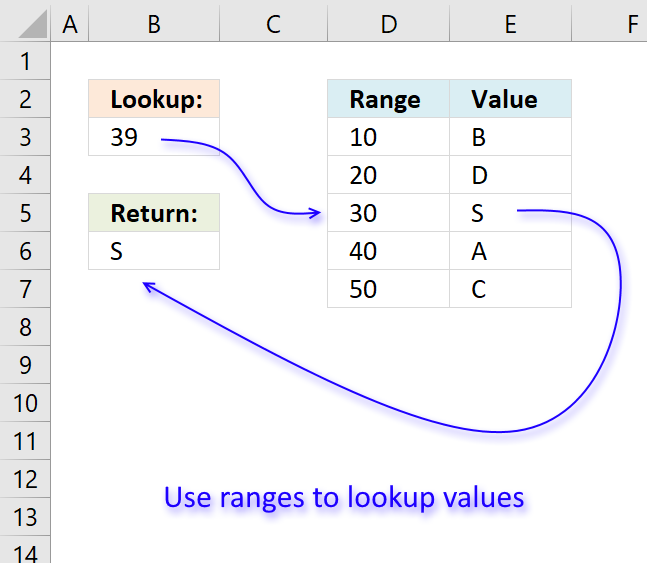
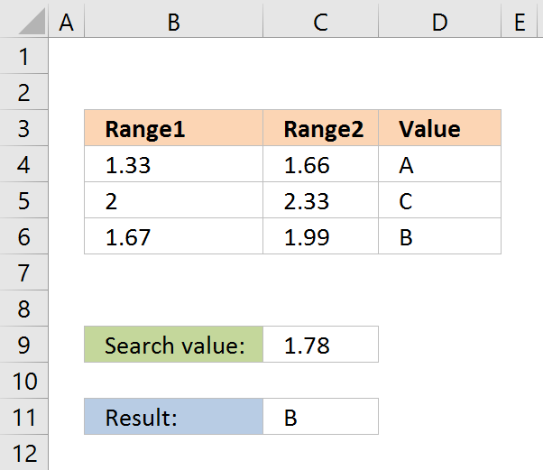
ie: Input Value 1.78 should return a Value of B as it is between the values in Range1 and Range2

Range1 Range2 Value
1.33 1.66 A
1.67 1.99 B
2.00 2.33 C

The next image shows the table in greater detail.

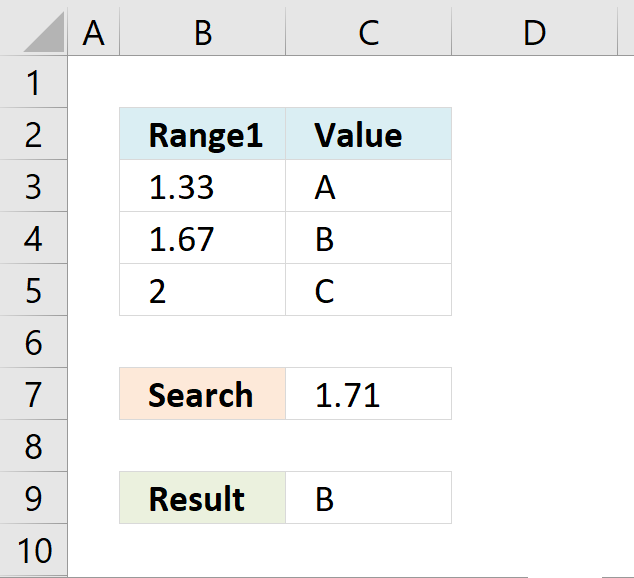
The picture above shows data in cell range B3:C5, the search value is in C7 and the result is in C9.

Cell range B3:B5 must be sorted in ascending order for the LOOKUP function to work properly.

Ascending order means values are sorted from the smallest to the largest value. Example: 1,5,8,11.

If an exact match is not found the largest value is returned as long as it is smaller than the lookup value.

The LOOKUP function then returns a value in a column on the same row.

The formula in cell C9:

=LOOKUP(C8,B4:B6,C4:C6)

Example, Search value 1.71 has no exact match, the largest value that is smaller than 1.71 is 1.67. The returning value is found in column C on the same row as 1.67, in this case, B.

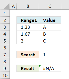If the search value is smaller than the smallest value in the lookup range the function returns #N/A meaning Not Available or does not exist.

Example in the picture to the right, search value is 1 in the and the LOOKUP function returns #N/A.

To solve this problem simply add another number, for example 0. Cell range B3:B6 would then contain 0, 1.33, 1.67, 2.

A search value greater than the largest value in the lookup range matches the largest value. Example in above picture, search value is 3 and the returning value is C.

Watch video below to see how the LOOKUP function works:

Learn more about the LOOKUP function, recommended reading:

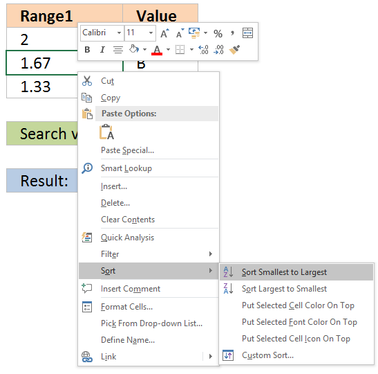
Tip! — You can quickly sort a cell range, follow these steps:

Press with right mouse button on on a cell in the cell range you want to sort
Hover with mouse cursor over Sort
Press with mouse on «Sort Smallest to Largest»

2. If the value is in the range then return value — INDEX + SUMPRODUCT + ROW

The following formula is slightly larger but you don’t need to sort cell range B4:B6.

The formula in cell C11:

=INDEX(D4:D6, SUMPRODUCT(—($D$8<=C4:C6), —($D$8>=B4:B6), ROW(A1:A3)))

The ranges don’t need to be sorted however you need a start (Range1) and an end value (Range2).

Explaining formula in cell C11

You can easily follow along, go to tab «Formulas» and press with left mouse button on «Evaluate Formula» button. Press with left mouse button on «Evaluate» button to move to next step.

Step 1 — Calculate first condition

The bolded part is the the logical expression I am going to explain in this step.

=INDEX(D4:D6, SUMPRODUCT(—($D$8<=C4:C6), —($D$8>=B4:B6), ROW(A1:A3)))

Logical operators

= equal sign
> less than sign
< greater than sign

The gretaer than sign combined with the equal sign <= means if value in cell D8 is smaller than or equal to the values in cell range C4:C6.

—($D$8<=C4:C6)

becomes

—(1,78<={1,66;1,99;2,33})

becomes

—{1,78<=1,66; 1,78<=1,99; 1,78<=2,33})

becomes

—({FALSE;TRUE;TRUE})

and returns {0;1;1}.

The double minus signs convert the boolean value TRUE or FALSE to the corresponding number 1 or 0 (zero).

Step 2 — Calculate second criterion

=INDEX(D4:D6, SUMPRODUCT(—($D$8<=C4:C6), —($D$8>=B4:B6), ROW(A1:A3)))

—($D$8>=B4:B6)

becomes

—(1,78>={1,33;1,67;2})

becomes

—({TRUE;TRUE;FALSE})

and returns

{1;1;0}

Step 3 — Create row numbers

=INDEX(D4:D6, SUMPRODUCT(—($D$8<=C4:C6), —($D$8>=B4:B6), ROW(A1:A3)))

ROW(A1:A3)

returns

{1;2;3}

Step 4 — Multiply criteria and row numbers and sum values

=INDEX(D4:D6, SUMPRODUCT(—($D$8<=C4:C6), —($D$8>=B4:B6), ROW(A1:A3)))

SUMPRODUCT(—($D$8<=C4:C6), —($D$8>=B4:B6), ROW(A1:A3))

becomes

SUMPRODUCT({0;1;1}, {1;1;0}, {1;2;3})

becomes

SUMPRODUCT({0;2;0})

and returns number 2.

Step 5 — Return a value of the cell at the intersection of a particular row and column

=INDEX(D4:D6, SUMPRODUCT(—($D$8<=C4:C6), —($D$8>=B4:B6), ROW(A1:A3)))

becomes

=INDEX(D4:D6, 2)

becomes

=INDEX({«A»;»B»;»C»}, 2)

and returns «B».

Functions in this formula: INDEX, SUMPRODUCT, ROW

3. If value in range then return value — VLOOKUP function

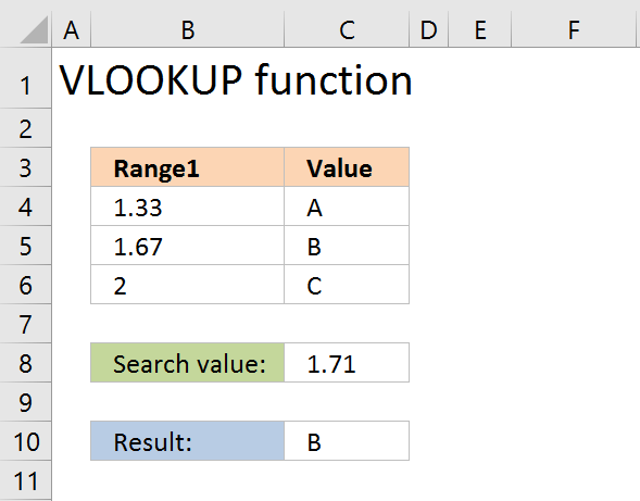
=VLOOKUP($D$8,$B$4:$D$6,3,TRUE)

The VLOOKUP function requires the table to be sorted based on range1 in an ascending order.

Explaining the VLOOKUP formula in cell C10

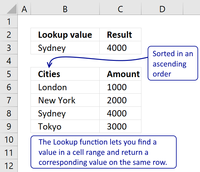
The VLOOKUP function looks for a value in the leftmost column of a table and then returns a value in the same row from a column you specify.

Arguments:
VLOOKUP(
lookup_value,
table_array,
col_index_num, [range_lookup]
)

The [range_lookup] argument is important in this case, it determines how the VLOOKUP function matches the lookup_value in the table_array.

The [range_lookup] is optional, it is either TRUE (default) or FALSE. It must be TRUE in our example here so that VLOOKUP returns an approximate match.

In order to do an approximate match the table_array must be sorted in an ascending order based on the first column.

=VLOOKUP($D$8,$B$4:$D$6,3,TRUE)

becomes

=VLOOKUP(1,78,{1,33, 1,66, «A»;1,67, 1,99, «B»;2, 2,33, «C»},3,TRUE)

1,67 is the next largest value and the VLOOKUP function returns «B».

4. If value in range then return value — INDEX + MATCH

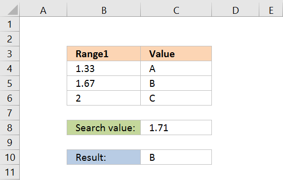
Formula in cell C10:

=INDEX($D$4:$D$6,MATCH(D8,$B$4:$B$6,1))

The lookup range must be sorted, just like the LOOKUP and VLOOKUP functions. Functions in this formula: INDEX and MATCH

Thanks JP!

Explaining INDEX+MATCH in cell D10

=INDEX($D$4:$D$6,MATCH(D8,$B$4:$B$6,1))

Step 1 — Return the relative position of an item in an array

The MATCH function returns the relative position of an item in an array or cell range that matches a specified value

Arguments:
MATCH(
lookup_value,
lookup_array,
[match_type])
)

The [match_type] argument is optional. It can be either -1, 0, or 1. 1 is default value if omitted.

The match_type argument determines how the MATCH function matches the lookup_value with values in lookup_array.

We want it to do an approximate search so I am going to use 1 as the argument.

This will make the MATCH find the largest value that is less than or equal to lookup_value. However, the values in the lookup_array argument must be sorted in an ascending order.

To learn more about the [match_type] argument read the article about the MATCH function.

=INDEX($D$4:$D$6,MATCH(D8,$B$4:$B$6,1))

MATCH(D8,$B$4:$B$6,1)

becomes

MATCH(1.78,{1.33;1.67;2},1)

1.67 is the largest value that is less than or equal to lookup_value. 1.67 is the second value in the array. MATCH function returns 2.

Step 2 — Return a value of the cell at the intersection of a particular row and column

=INDEX($D$4:$D$6,MATCH(D8,$B$4:$B$6,1))

becomes

=INDEX($D$4:$D$6,2)

becomes

=INDEX({«A»;»B»;»C»},2)

and returns «B».

Quickly lookup a value in a numerical range

You can also do lookups in date ranges, dates in Excel are actually numbers.

Источник

This post will guide you how to return a value if a cell contains a certain number or text string in Excel. How do I check if a Cell contains specific text and then return another specific text in another cell with a formula in Excel.

Return Value If Cell Contains Certain Value
Video: Return Value If Cell Contains Certain Value

Table of Contents

Return Value If Cell Contains Certain Value
- Related Functions

Assuming that you want to check if a given Cell such as B1 contains a text string “excel”, if True, returns another text string “learning excel” in Cell C1. How to achieve it. You can use a formula based on the IF function, the ISNUMBER function and the SEARCH function to achieve the result of return a value if Cell contains a specific value. Just like this:

=IF(ISNUMBER(SEARCH("excel",B1)),"learning excel","")

Type this formula into the formula box of cell C1, and then press Enter key in your keyboard.

return value if cell contains certain value1

You will see that the text string “learning excel” will be returned in the Cell C1.

And if you want to check the range of cells B1:B4, you need to drag the AutoFill Handle down to other cells to apply this formula.

return value if cell contains certain value2

Video: Return Value If Cell Contains Certain Value

Excel SEARCH function
The Excel SEARCH function returns the number of the starting location of a substring in a text string.The syntax of the SEARCH function is as below:= SEARCH (find_text, within_text,[start_num])…
Excel ISNUMBER function
The Excel ISNUMBER function returns TRUE if the value in a cell is a numeric value, otherwise it will return FALSE.The syntax of the ISNUMBER function is as below:= ISNUMBER (value)…
Excel IF function
The Excel IF function perform a logical test to return one value if the condition is TRUE and return another value if the condition is FALSE.The syntax of the IF function is as below:= IF (condition, [true_value], [false_value])…

Источник

Tip

Insert Line Break in Excel

Wrapping Text in Excel

What is Carriage Return in Excel Cell?

Table of contents

How to Insert a Carriage Return in Excel?

Insert Excel Carriage Return by using Formula

How to Remove Carriage Return Character from Excel Cell?

Things to Remember

Recommended Articles

Method 1 — Cell Wrapping

Method 2 — Insert a Return

Method 3 — Using a Formula

Lookup And Return Cell Address Using the ADDRESS Function

Lookup And Return Cell Address Using the CELL Function

What’s on this page

1. If value in range then return value — LOOKUP function

Tip! — You can quickly sort a cell range, follow these steps:

2. If the value is in the range then return value — INDEX + SUMPRODUCT + ROW

Explaining formula in cell C11

3. If value in range then return value — VLOOKUP function

Explaining the VLOOKUP formula in cell C10

4. If value in range then return value — INDEX + MATCH

Explaining INDEX+MATCH in cell D10

Quickly lookup a value in a numerical range