
Содержание
- How to return an entire column
- Syntax
- Steps
- INDEX
- OFFSET
- Return in excel column
- What’s on this page
- 1. If value in range then return value — LOOKUP function
- Tip! — You can quickly sort a cell range, follow these steps:
- 2. If the value is in the range then return value — INDEX + SUMPRODUCT + ROW
- Explaining formula in cell C11
- 3. If value in range then return value — VLOOKUP function
- Explaining the VLOOKUP formula in cell C10
- 4. If value in range then return value — INDEX + MATCH
- Explaining INDEX+MATCH in cell D10
- Get the Excel file
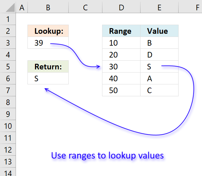
- Quickly lookup a value in a numerical range
- How to Return the Column Letter (Not Number) With Excel Function
- Summary
- Introduction: Return the column number
- Built-in Excel function to return the column letter from cell
- Even easier: Use Professor Excel Tools to return the column letter
How to return an entire column

To return an entire column you need array returning functions like INDEX or OFFSET. Both of these functions can return arrays, as well as single values, which can be used in other functions like SUM, AVERAGE or even another INDEX or OFFSET. How to return an entire column article will explain you how it can be done.
Syntax
=INDEX(data without headers, 0, MATCH(search value, headers of data, 0))
=OFFSET(anchor point before headers, 1, MATCH(search value, headers of data, 0), ROWS(any column of data or even data itself), 1)
Steps
- Start with =INDEX( which returns the range
- Type or select the range includes data C3:E7,
- Continue with 0, to specify that you want entire column
- Use MATCH( to find location of desired column
- Select the range which includes the value that specifies the column H3,
- Select the range which includes the value that includes the headers C2:E2,
- Type 0)) to select the exact match method and close both INDEX and MATCH formulas
As it is mentioned above, to return an entire column or row, you need to use array returning functions. An alternative way may be to use array functions. However, in most occasions they are fairly complex, unnecessary (due to existing formulas) and run slower.
The INDEX and OFFSET are powerful functions to return a value or range when they are combined with MATCH function which can handle the lookup process. Let’s see how they work:
INDEX
The trick is to use «0″ as row argument which specifies that you want to entire column in data instead of a single cell. The rest is how it is done with regular INDEX-MATCH. So use the MATCH function to find the location of a column:
The INDEX function will return an array which includes values in that column.
What Excel displays: 71
Please note that Excel will show only the first value of the array if you do not them in another formula. We used the AVERAGE function to demonstrate how the array can be used.
OFFSET
The OFFSET function uses a similar approach as well. Instead of INDEX that you need to select whole data range, the OFFSET function requires the cell outside of the data range which can be used as an anchor point.
Another difference is the OFFSET returns an array when its optional arguments are used. These arguments basically represents the size of rows and columns to return.
Briefly; you need to specify where the column starts and how long it is. The MATCH function works the same as before to lookup the column we need and the ROWS function returns the column length. Of course we used «1» as row number because we only need a single column.
Источник
Return in excel column
In this article, I will demonstrate four different formulas that allow you to lookup a value that is to be found in a given range and return the corresponding value on the same row. If you need to return multiple values because the ranges overlap then read this article: Return multiple values if in range.
What’s on this page
They all have their pros and cons and I will discuss those in great detail, they can be applied to not only numerical ranges but also text ranges and date ranges as well.
I have made a video that explains the LOOKUP function in context to this article, if you are interested.
There is a file for you to get, at the end of this article, which contains all the formula examples in a worksheet each.
Check out the LOOKUP category to find more interesting articles.
The following table shows the differences between the formulas presented in this article.
| Formula | Range sorted? | Array formula | Get value from any column? | Two range columns? |
| LOOKUP | Yes | No | Yes | No |
| INDEX + SUMPRODUCT + ROW | No | No | Yes | Yes |
| VLOOKUP | Yes | No | No | No |
| INDEX + MATCH | Yes | No | Yes | No |
Some formulas require you to have the lookup range sorted to function properly, the INDEX+SUMPRODUCT+ROW alternative is the only way to go if you can’t sort the values.
The disadvantage with the INDEX+SUMPRODUCT+ROW formula is that you need start and end values, the other formulas use the start values also as end range values.
The VLOOKUP function can only search the leftmost column, you must rearrange your table to meet this condition if you are going to use the VLOOKUP function.
1. If value in range then return value — LOOKUP function
To better demonstrate the LOOKUP function I am going to answer the following question.
What type of formula could be used if you weren’t using a date range and your data was not concatenated?
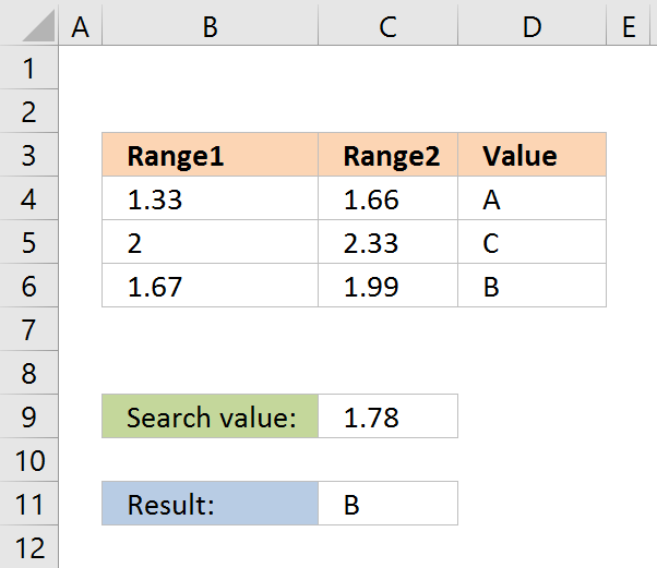
ie: Input Value 1.78 should return a Value of B as it is between the values in Range1 and Range2
Range1 Range2 Value
1.33 1.66 A
1.67 1.99 B
2.00 2.33 C
The next image shows the table in greater detail.
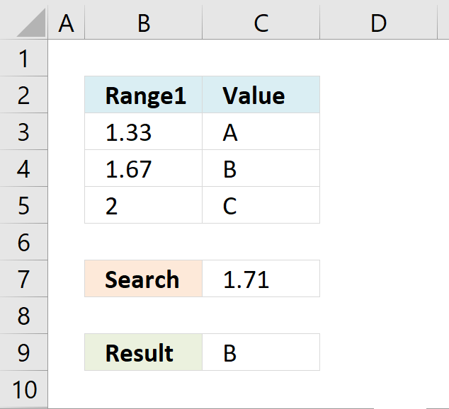
The picture above shows data in cell range B3:C5, the search value is in C7 and the result is in C9.
Cell range B3:B5 must be sorted in ascending order for the LOOKUP function to work properly.
If an exact match is not found the largest value is returned as long as it is smaller than the lookup value.
The LOOKUP function then returns a value in a column on the same row.
The formula in cell C9:
Example, Search value 1.71 has no exact match, the largest value that is smaller than 1.71 is 1.67. The returning value is found in column C on the same row as 1.67, in this case, B.
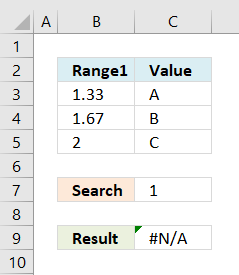 If the search value is smaller than the smallest value in the lookup range the function returns #N/A meaning Not Available or does not exist.
Example in the picture to the right, search value is 1 in the and the LOOKUP function returns #N/A.
To solve this problem simply add another number, for example 0. Cell range B3:B6 would then contain 0, 1.33, 1.67, 2.
A search value greater than the largest value in the lookup range matches the largest value. Example in above picture, search value is 3 and the returning value is C.
Watch video below to see how the LOOKUP function works:
Learn more about the LOOKUP function, recommended reading:
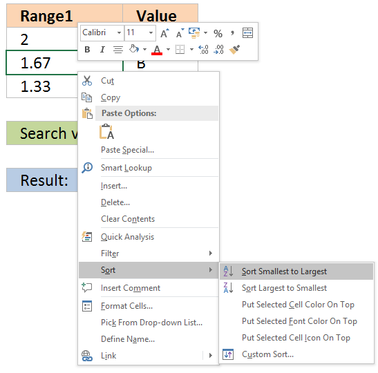
Tip! — You can quickly sort a cell range, follow these steps:
- Press with right mouse button on on a cell in the cell range you want to sort

- Hover with mouse cursor over Sort
- Press with mouse on «Sort Smallest to Largest»
2. If the value is in the range then return value — INDEX + SUMPRODUCT + ROW
The following formula is slightly larger but you don’t need to sort cell range B4:B6.
The formula in cell C11:
The ranges don’t need to be sorted however you need a start (Range1) and an end value (Range2).
Explaining formula in cell C11
You can easily follow along, go to tab «Formulas» and press with left mouse button on «Evaluate Formula» button. Press with left mouse button on «Evaluate» button to move to next step.
Step 1 — Calculate first condition
The bolded part is the the logical expression I am going to explain in this step.
=INDEX(D4:D6, SUMPRODUCT(—($D$8 =B4:B6), ROW(A1:A3)))
Logical operators
= equal sign
> less than sign
=B4:B6), ROW(A1:A3)))
Step 3 — Create row numbers
=INDEX(D4:D6, SUMPRODUCT(—($D$8 =B4:B6), ROW(A1:A3)))
Step 4 — Multiply criteria and row numbers and sum values
=INDEX(D4:D6, SUMPRODUCT(—($D$8 =B4:B6), ROW(A1:A3)))
SUMPRODUCT(—($D$8 =B4:B6), ROW(A1:A3))
and returns number 2.
Step 5 — Return a value of the cell at the intersection of a particular row and column
=INDEX(D4:D6, SUMPRODUCT(—($D$8 =B4:B6), ROW(A1:A3)))
Functions in this formula: INDEX, SUMPRODUCT, ROW
3. If value in range then return value — VLOOKUP function
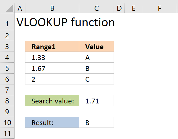
The VLOOKUP function requires the table to be sorted based on range1 in an ascending order.
Explaining the VLOOKUP formula in cell C10
The VLOOKUP function looks for a value in the leftmost column of a table and then returns a value in the same row from a column you specify.
The [range_lookup] argument is important in this case, it determines how the VLOOKUP function matches the lookup_value in the table_array.
The [range_lookup] is optional, it is either TRUE (default) or FALSE. It must be TRUE in our example here so that VLOOKUP returns an approximate match.
In order to do an approximate match the table_array must be sorted in an ascending order based on the first column.
1,67 is the next largest value and the VLOOKUP function returns «B».
4. If value in range then return value — INDEX + MATCH
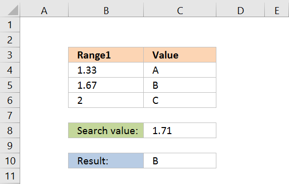
Formula in cell C10:
The lookup range must be sorted, just like the LOOKUP and VLOOKUP functions. Functions in this formula: INDEX and MATCH
Thanks JP!
Explaining INDEX+MATCH in cell D10
Step 1 — Return the relative position of an item in an array
The MATCH function returns the relative position of an item in an array or cell range that matches a specified value
The [match_type] argument is optional. It can be either -1, 0, or 1. 1 is default value if omitted.
The match_type argument determines how the MATCH function matches the lookup_value with values in lookup_array.
We want it to do an approximate search so I am going to use 1 as the argument.
This will make the MATCH find the largest value that is less than or equal to lookup_value. However, the values in the lookup_array argument must be sorted in an ascending order.
To learn more about the [match_type] argument read the article about the MATCH function.
1.67 is the largest value that is less than or equal to lookup_value. 1.67 is the second value in the array. MATCH function returns 2.
Step 2 — Return a value of the cell at the intersection of a particular row and column
Get the Excel file
Quickly lookup a value in a numerical range
You can also do lookups in date ranges, dates in Excel are actually numbers.
Источник
How to Return the Column Letter (Not Number) With Excel Function

There are a few cases in Excel when you need to return the column letter from an Excel cell. For example, when you use the INDIRECT function. Retrieving the number of a cell is quite simple using the =COLUMN() function. But the letter? Here is how to do that!
Summary
In a hurry? Copy and paste this function and replace “B5” with the cell you want to return the column letter from:
Introduction: Return the column number
Before we start, a small introduction of the simple =COLUMN() function in Excel. It returns the column number and is quite simple:
This function returns the column number of cell B5 – so the result is 2 because column B is the second column.
You can also use this function without any argument:
This way, the function returns the column number of the current column.
Built-in Excel function to return the column letter from cell
We have seen above how to return the column number. Let’s take the next step now and return the column letter. I’m going to introduce you to the easiest method – of course, there are multiple options.
This version involves the ADDRESS function as well as the SUBSTITUE function. With the ADDRESS function we return the column letter as well as number and with the SUBSTITUTE function we remove the number from it.
The whole function is:
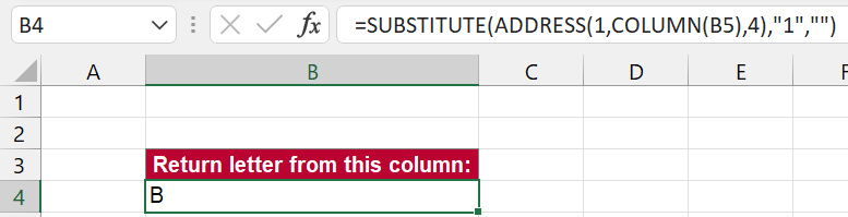 Return the column letter with this function in Excel.
The key of this function is that the ADDRESS function converts the “coordinates” of a cell to letter and number. So, let’s only talk about the ADDRESS function now:
- The first argument (1) is the row number. We set it to row number 1 and later on remove it with the SUBSTITUTE function.
- As seen above, the COLUMN(B5) argument returns two and defines the column number in the ADDRESS function.
- The number 4 as the third argument just defines the address style. Number 4 means a relative reference without any dollar signs.
That means, the ADDRESS function in this case returns “B1”. With the SUBSTITUTE function wrapped around we remove the one so that the final result is only “B”.
If you want to return the column letter of the current column, you can simply remove the B5. The function is:
If you have Professor Excel Tools already, you can simply use the =PROFEXColumn() function to return the column letter.
In this case, it is:
For using the PROFEX functions you don’t have to purchase a license. In order to maximize the compatibility, all functions starting with =PROFEX are free to use.
Even better: If you click on the fx button on the Professor Excel ribbon and insert the function here, it will automatically converted to built-in Excel function:
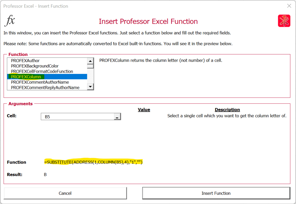 When you insert the PROFEXColumn function to return the column letter via the fx window, it will automatically be converted to Excel built-in functions.

This function is included in our Excel Add-In ‘Professor Excel Tools’
(No sign-up, download starts directly)
More than 35,000 users can’t be wrong.
Источник
VLOOKUP is one of the most used functions in Excel. It looks for a value in a range and returns a corresponding value in a specified column number.
Now I came across a problem where I had to lookup entire row and return the values in all the columns from that row (instead of returning a single value).
So here is what I had to do. In the below dataset, I had Sales Rep names and the Sales they made in 4 quarters in 2012. I had a drop down with their names, and I wanted to extract the maximum sales for that Sales Rep in those four quarters.

I could come up with 2 different ways to do this – Using INDEX or VLOOKUP.
Lookup Entire Row / Column Using INDEX Formula
Here is the formula I created to do this using Index
=LARGE(INDEX($B$4:$F$13,MATCH(H3,$B$4:$B$13,0),0),1)
How it works:
Let first look at the INDEX function that is wrapped inside the LARGE function.
=INDEX($C$4:$F$13,MATCH(H3,$B$4:$B$13,0),0)
Let’s closely analyze the arguments of the INDEX function:
- Array – $B$4:$F$1
- Row Number – MATCH(H3,$B$4:$B$13,0)
- Column Number – 0
Notice that I have used column number as 0.
The trick here is that when you use column number as 0, it returns all the values in all the columns. So if I select John in the drop down, the index formula would return all the 4 sales values for John {91064,71690,67574,25427}.
Now I can use the Large function to extract the largest value
Pro Tip - Use Column/Row number as 0 in Index formula to return all the values in Columns/Rows.
Lookup Entire Row / Column Using VLOOKUP Formula
While Index formula is neat, clean and robust, VLOOKUP way is a bit complex. It also ends up making the function volatile. However, there is an amazing trick that I would share in this section. Here is the formula:
=LARGE(VLOOKUP(H3,B4:F13, ROW(INDIRECT("2:"&COUNTA($B$4:$F$4))), FALSE),1)
How it works
- ROW(INDIRECT(“2:”&COUNTA($B$4:$F$4))) – This formula returns an array {2;3;4;5}. Note that since it uses INDIRECT, this makes this formula volatile.
- VLOOKUP(H3,B4:F13,ROW(INDIRECT(“2:”&COUNTA($B$4:$F$4))),FALSE) – Here is the best part. When you put these together, it becomes VLOOKUP(H3,B4:F13,{2;3;4;5},FALSE). Now notice that instead of a single column number, I have given it an array of column numbers. And VLOOKUP obediently looks up values in all these columns and returns an array.
- Now just use LARGE function to extract the largest value.
Remember to use Control + Shift + Enter to use this formula.
Pro Tip - In VLOOKUP, instead of using a single column number, if you use an array of column numbers, it will return an array of lookup values.
You may also like the following Excel tutorials:
- VLOOKUP Vs. INDEX/MATCH
- How to make VLOOKUP Case Sensitive.
- How to Use VLOOKUP with Multiple Criteria.
- How to Sum a Column in Excel
- How to Return Cell Address Instead of Value in Excel
- How to Apply Formula to the Entire Column in Excel
To return an entire column you need array returning functions like INDEX or OFFSET. Both of these functions can return arrays, as well as single values, which can be used in other functions like SUM, AVERAGE or even another INDEX or OFFSET. How to return an entire column article will explain you how it can be done.
Syntax
=INDEX(data without headers, 0, MATCH(search value, headers of data, 0))
=OFFSET(anchor point before headers, 1, MATCH(search value, headers of data, 0), ROWS(any column of data or even data itself), 1)
Steps
- Start with =INDEX( which returns the range
- Type or select the range includes data C3:E7,
- Continue with 0, to specify that you want entire column
- Use MATCH( to find location of desired column
- Select the range which includes the value that specifies the column H3,
- Select the range which includes the value that includes the headers C2:E2,
- Type 0)) to select the exact match method and close both INDEX and MATCH formulas
How
As it is mentioned above, to return an entire column or row, you need to use array returning functions. An alternative way may be to use array functions. However, in most occasions they are fairly complex, unnecessary (due to existing formulas) and run slower.
The INDEX and OFFSET are powerful functions to return a value or range when they are combined with MATCH function which can handle the lookup process. Let’s see how they work:
INDEX
The trick is to use «0″ as row argument which specifies that you want to entire column in data instead of a single cell. The rest is how it is done with regular INDEX-MATCH. So use the MATCH function to find the location of a column:
MATCH(H3,C2:E2,0)
The INDEX function will return an array which includes values in that column.
The result: {71;64;56;80;80}
What Excel displays: 71
Please note that Excel will show only the first value of the array if you do not them in another formula. We used the AVERAGE function to demonstrate how the array can be used.
=AVERAGE(INDEX(C3:E7,0,MATCH(H3,C2:E2,0)))
The result: 70.2
OFFSET
The OFFSET function uses a similar approach as well. Instead of INDEX that you need to select whole data range, the OFFSET function requires the cell outside of the data range which can be used as an anchor point.
Another difference is the OFFSET returns an array when its optional arguments are used. These arguments basically represents the size of rows and columns to return.
Briefly; you need to specify where the column starts and how long it is. The MATCH function works the same as before to lookup the column we need and the ROWS function returns the column length. Of course we used «1» as row number because we only need a single column.
=AVERAGE(OFFSET(B2,1,MATCH(H3,C2:E2,0),ROWS(B3:B7),1))
Author: Oscar Cronquist Article last updated on February 17, 2023
In this article, I will demonstrate four different formulas that allow you to lookup a value that is to be found in a given range and return the corresponding value on the same row. If you need to return multiple values because the ranges overlap then read this article: Return multiple values if in range.
What’s on this page
- If value in range then return value — LOOKUP function
- If value in range then return value — INDEX + SUMPRODUCT + ROW
- If value in range then return value — VLOOKUP function
- If value in range then return value — INDEX + MATCH
They all have their pros and cons and I will discuss those in great detail, they can be applied to not only numerical ranges but also text ranges and date ranges as well.
I have made a video that explains the LOOKUP function in context to this article, if you are interested.
There is a file for you to get, at the end of this article, which contains all the formula examples in a worksheet each.
You can use the techniques described in this article to calculate discount percentages based on price intervals or linear results based on the lookup value.
Check out the LOOKUP category to find more interesting articles.
The following table shows the differences between the formulas presented in this article.
| Formula | Range sorted? | Array formula | Get value from any column? | Two range columns? |
| LOOKUP | Yes | No | Yes | No |
| INDEX + SUMPRODUCT + ROW | No | No | Yes | Yes |
| VLOOKUP | Yes | No | No | No |
| INDEX + MATCH | Yes | No | Yes | No |
Some formulas require you to have the lookup range sorted to function properly, the INDEX+SUMPRODUCT+ROW alternative is the only way to go if you can’t sort the values.
The disadvantage with the INDEX+SUMPRODUCT+ROW formula is that you need start and end values, the other formulas use the start values also as end range values.
The VLOOKUP function can only search the leftmost column, you must rearrange your table to meet this condition if you are going to use the VLOOKUP function.
1. If value in range then return value — LOOKUP function
To better demonstrate the LOOKUP function I am going to answer the following question.
Hi,
What type of formula could be used if you weren’t using a date range and your data was not concatenated?
ie: Input Value 1.78 should return a Value of B as it is between the values in Range1 and Range2
Range1 Range2 Value
1.33 1.66 A
1.67 1.99 B
2.00 2.33 C
The next image shows the table in greater detail.
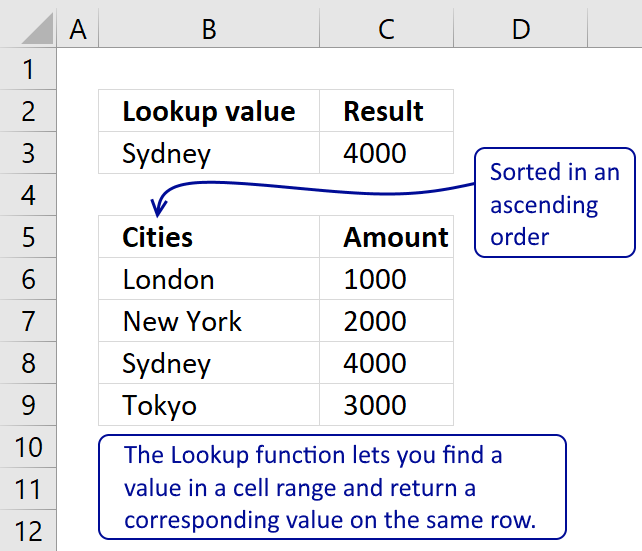
The picture above shows data in cell range B3:C5, the search value is in C7 and the result is in C9.
Cell range B3:B5 must be sorted in ascending order for the LOOKUP function to work properly.
Ascending order means values are sorted from the smallest to the largest value. Example: 1,5,8,11.
If an exact match is not found the largest value is returned as long as it is smaller than the lookup value.
The LOOKUP function then returns a value in a column on the same row.
The formula in cell C9:
=LOOKUP(C8,B4:B6,C4:C6)
Example, Search value 1.71 has no exact match, the largest value that is smaller than 1.71 is 1.67. The returning value is found in column C on the same row as 1.67, in this case, B.
If the search value is smaller than the smallest value in the lookup range the function returns #N/A meaning Not Available or does not exist.
Example in the picture to the right, search value is 1 in the and the LOOKUP function returns #N/A.
To solve this problem simply add another number, for example 0. Cell range B3:B6 would then contain 0, 1.33, 1.67, 2.
A search value greater than the largest value in the lookup range matches the largest value. Example in above picture, search value is 3 and the returning value is C.
Watch video below to see how the LOOKUP function works:
Learn more about the LOOKUP function, recommended reading:
Recommended articles
Tip! — You can quickly sort a cell range, follow these steps:
- Press with right mouse button on on a cell in the cell range you want to sort

- Hover with mouse cursor over Sort
- Press with mouse on «Sort Smallest to Largest»
Back to top
2. If the value is in the range then return value — INDEX + SUMPRODUCT + ROW
The following formula is slightly larger but you don’t need to sort cell range B4:B6.
The formula in cell C11:
=INDEX(D4:D6, SUMPRODUCT(—($D$8<=C4:C6), —($D$8>=B4:B6), ROW(A1:A3)))
The ranges don’t need to be sorted however you need a start (Range1) and an end value (Range2).
Back to top
Explaining formula in cell C11
You can easily follow along, go to tab «Formulas» and press with left mouse button on «Evaluate Formula» button. Press with left mouse button on «Evaluate» button to move to next step.
Step 1 — Calculate first condition
The bolded part is the the logical expression I am going to explain in this step.
=INDEX(D4:D6, SUMPRODUCT(—($D$8<=C4:C6), —($D$8>=B4:B6), ROW(A1:A3)))
Logical operators
= equal sign
> less than sign
< greater than sign
The gretaer than sign combined with the equal sign <= means if value in cell D8 is smaller than or equal to the values in cell range C4:C6.
—($D$8<=C4:C6)
becomes
—(1,78<={1,66;1,99;2,33})
becomes
—{1,78<=1,66; 1,78<=1,99; 1,78<=2,33})
becomes
—({FALSE;TRUE;TRUE})
and returns {0;1;1}.
The double minus signs convert the boolean value TRUE or FALSE to the corresponding number 1 or 0 (zero).
Step 2 — Calculate second criterion
=INDEX(D4:D6, SUMPRODUCT(—($D$8<=C4:C6), —($D$8>=B4:B6), ROW(A1:A3)))
—($D$8>=B4:B6)
becomes
—(1,78>={1,33;1,67;2})
becomes
—({TRUE;TRUE;FALSE})
and returns
{1;1;0}
Step 3 — Create row numbers
=INDEX(D4:D6, SUMPRODUCT(—($D$8<=C4:C6), —($D$8>=B4:B6), ROW(A1:A3)))
ROW(A1:A3)
returns
{1;2;3}
Step 4 — Multiply criteria and row numbers and sum values
=INDEX(D4:D6, SUMPRODUCT(—($D$8<=C4:C6), —($D$8>=B4:B6), ROW(A1:A3)))
SUMPRODUCT(—($D$8<=C4:C6), —($D$8>=B4:B6), ROW(A1:A3))
becomes
SUMPRODUCT({0;1;1}, {1;1;0}, {1;2;3})
becomes
SUMPRODUCT({0;2;0})
and returns number 2.
Step 5 — Return a value of the cell at the intersection of a particular row and column
=INDEX(D4:D6, SUMPRODUCT(—($D$8<=C4:C6), —($D$8>=B4:B6), ROW(A1:A3)))
becomes
=INDEX(D4:D6, 2)
becomes
=INDEX({«A»;»B»;»C»}, 2)
and returns «B».
Functions in this formula: INDEX, SUMPRODUCT, ROW
Back to top
3. If value in range then return value — VLOOKUP function
=VLOOKUP($D$8,$B$4:$D$6,3,TRUE)
The VLOOKUP function requires the table to be sorted based on range1 in an ascending order.
Back to top
Explaining the VLOOKUP formula in cell C10
The VLOOKUP function looks for a value in the leftmost column of a table and then returns a value in the same row from a column you specify.
Arguments:
VLOOKUP(
lookup_value,
table_array,
col_index_num, [range_lookup]
)
The [range_lookup] argument is important in this case, it determines how the VLOOKUP function matches the lookup_value in the table_array.
The [range_lookup] is optional, it is either TRUE (default) or FALSE. It must be TRUE in our example here so that VLOOKUP returns an approximate match.
In order to do an approximate match the table_array must be sorted in an ascending order based on the first column.
=VLOOKUP($D$8,$B$4:$D$6,3,TRUE)
becomes
=VLOOKUP(1,78,{1,33, 1,66, «A»;1,67, 1,99, «B»;2, 2,33, «C»},3,TRUE)
1,67 is the next largest value and the VLOOKUP function returns «B».
Back to top
4. If value in range then return value — INDEX + MATCH
Formula in cell C10:
=INDEX($D$4:$D$6,MATCH(D8,$B$4:$B$6,1))
The lookup range must be sorted, just like the LOOKUP and VLOOKUP functions. Functions in this formula: INDEX and MATCH
Thanks JP!
Back to top
Explaining INDEX+MATCH in cell D10
=INDEX($D$4:$D$6,MATCH(D8,$B$4:$B$6,1))
Step 1 — Return the relative position of an item in an array
The MATCH function returns the relative position of an item in an array or cell range that matches a specified value
Arguments:
MATCH(
lookup_value,
lookup_array,
[match_type])
)
The [match_type] argument is optional. It can be either -1, 0, or 1. 1 is default value if omitted.
The match_type argument determines how the MATCH function matches the lookup_value with values in lookup_array.
We want it to do an approximate search so I am going to use 1 as the argument.
This will make the MATCH find the largest value that is less than or equal to lookup_value. However, the values in the lookup_array argument must be sorted in an ascending order.
To learn more about the [match_type] argument read the article about the MATCH function.
=INDEX($D$4:$D$6,MATCH(D8,$B$4:$B$6,1))
MATCH(D8,$B$4:$B$6,1)
becomes
MATCH(1.78,{1.33;1.67;2},1)
1.67 is the largest value that is less than or equal to lookup_value. 1.67 is the second value in the array. MATCH function returns 2.
Step 2 — Return a value of the cell at the intersection of a particular row and column
=INDEX($D$4:$D$6,MATCH(D8,$B$4:$B$6,1))
becomes
=INDEX($D$4:$D$6,2)
becomes
=INDEX({«A»;»B»;»C»},2)
and returns «B».
Back to top
Back to top
Quickly lookup a value in a numerical range
You can also do lookups in date ranges, dates in Excel are actually numbers.

No one wants to jump through hoops to get the job done, but sometimes a simple solution can elude us. If the answer isn’t quick and easy, we often turn to complex array functions or code believing there’s no other way. A good example is trying to return the last value in a column, conditionally, because the matching row won’t always be the last row. Throwing that condition into the mix seems to make things much harder. In this article, I’ll show you a couple of simple methods that work, but they’re not superior solutions. Then, I’ll show you a more dynamic solution that requires only a bit more work.
I’m using Microsoft 365 on a Windows 10 64-bit solution, but you can use earlier versions. You can work with your own data or download the demonstration .xlsx file and .xls files. However, the menu version doesn’t support the Table object needed in the Dynamic section. This article assumes you have basic Excel skills such as filtering and entering functions. The browser edition supports everything in this article.
SEE: Excel power user guide (TechRepublic Premium)
Defining the term last
We know what the word last means, but defining it within the context of the data is important. Do we mean the last matching record in the data set? Do we mean the latest date? Or do we mean the least value? Looking over our simple data set, you can see that the answer to all three questions could be yes (Figure A).
Figure A

Practically speaking, we can eliminate the least and date values, because you’d be looking for a minimum value, and that’s not really the same thing as the last value. So that leaves us with the last record that matches the condition.
Simple, but not dynamic
We have two vendors, Acme and ABC, Inc., and let’s suppose we want to return the date and invoice amount for the last record in the data set for each company. You might think of VLOOKUP(), but that function returns the first matching value. There’s no way to force the function to find the last matching value.
If you control the data, you have an easy solution—reverse the records and use VLOOKUP(), which with a reversed data set, will find the last (first) record. The easiest way to reverse the record order is to populate a helper column with a set of consecutive numbers (Figure B).
Figure B

Next, let’s add the VLOOKUP() functions for returning the date and invoice (see Figure B). There are two lookup functions and the only difference between them is the return column:
G3: =VLOOKUP($F3,$B$3:$D$18,3,FALSE)
H3: =VLOOKUP($F3,$B$3:$D$18,2,FALSE)
Copy the functions in row 3 to row 4. Right now, these functions return the first matching record for both companies. To get the last, reverse the data set by running a descending sort on the helper column you added. Figure C shows the results; now the VOOKUP() functions return the values for the “last” matching record. This is a simple solution, but it isn’t dynamic; you must remember to sort, which isn’t ideal.
Figure C

A simple filter will give you a quick visual (Figure D), if that’s all you need. To do so, click anywhere inside the data set and then click the Data tab. In the Sort & Filter group, click Filter. Then, use the dropdown list for the Vendor column and select only one company at a time.
Figure D

Dynamic
The VLOOKUP() and filter solutions are only partial solutions—having to remember to sort or getting just a visual clue isn’t enough. We can combine both partial solutions to create a good one that is dynamic and requires no extra action on your part other than filtering the data set. Using this solution, you can’t get both sets of data at the same time, but you might find it works better for you than the above solutions.
I’ve added a filtering row above the data set, and turned the data set into a Table object with a Totals row (Figure E). To create the Table, click any cell inside the data range, press Ctrl+t and click OK. To add the Totals row, click the contextual Table Design ribbon and check the Total Row option in the Table Style Options group. Finally, click inside the Order columns total cell—in the example sheet, that’s A20—and select Max from the dropdown. Doing so returns the maximum number in that column. Remember, the menu version doesn’t support the Table object.
Figure E

To create the filtering row, add the functions as follows:
A1: =Table2[[#Totals],[Order]]
B1: =VLOOKUP($A$1,Table2,2,FALSE)
C1: =VLOOKUP($A$1,Table2,3,FALSE)
D1: =VLOOKUP($A$1,Table2,4,FALSE)
As before, the VLOOKUP() function still finds the first matching value in the respective columns. The main difference is that the reference to the lookup table is a reference to Table2 (the Table we created). The expression in A1 references the value in the totals row for the Order column. That value is the result of a special SUBTOTAL() function that returns the maximum value in the filtered set.
In other words, the lookup value for the VLOOKUP() function is the value in A20—the largest value in the filtered set. Consequently, the function returns the corresponding values from that row.
With no filter in place, the filtering row always return the last row of values. Now let’s see what happens when we filter by company. To do so, choose only one company at a time from the Vendor columns dropdown. As you can see in Figure F, the filtered set for Acme returns the same values as a non-filtered set—that’s because the last row in the data set is an Acme record.
Figure F

Figure G shows the results of filtering for ABC, Inc. This time, the data changes to reflect the last record for that vendor.
Figure G

You still must filter the set to get the correct results in row A, but that’s much easier to remember than the sorting business from the earlier solution.
This tutorial will demonstrate how to return multiple columns using XLOOKUP in Excel. If your version of Excel does not support XLOOKUP, read how to return multiple columns using VLOOKUP instead.
XLOOKUP Return Consecutive Columns
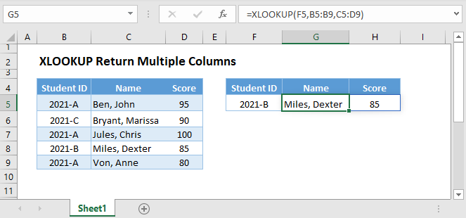
One advantage of the XLOOKUP Function is that it can return multiple consecutive columns at once. To do this, input the range of consecutive columns in the return array, and it will return all the columns.
=XLOOKUP(F3,B3:B7,C3:D7)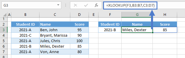
Notice here our return array is two columns (C and D), and thus 2 columns are returned.
XLOOKUP-FILTER Return Non-Adjacent Columns
Although the XLOOKUP Function can return multiple consecutive columns, it can’t return non-adjacent columns. To return non-adjacent columns, we can use the FILTER Function.
=XLOOKUP(F3,C3:C7,FILTER(B3:D7,{1,0,1}))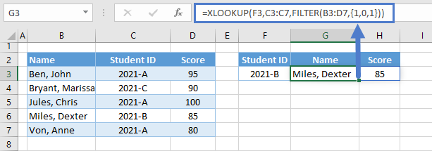
Let’s walk through the formula:
FILTER Function
The FILTER Function is commonly used for filtering rows, but it can also be used for filtering columns. To do this, we input a horizontal array of 1s (TRUE) and 0s (FALSE) with the same no. of columns from the array input (1st argument). Columns that match with 0s are filtered out while columns that match with 1s are returned.
=FILTER(B3:D7,{1,0,1})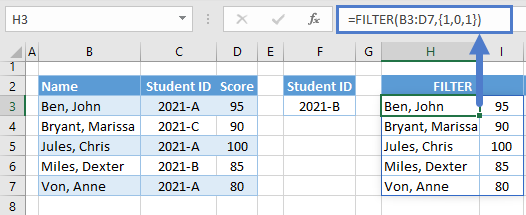
XLOOKUP Function
The output of the FILTER Function is then used as the return array of our XLOOKUP.
=XLOOKUP(F3,C3:C7,H3:I7)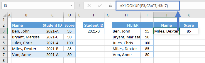
Combining all functions together yields our original formula:
=XLOOKUP(F3,C3:C7,FILTER(B3:D7,{1,0,1}))XLOOKUP-FILTER-COUNTIF Return Non-Adjacent Columns
Instead of manually selecting the columns to be filtered out, we can use the COUNTIF Function to automatically determine the columns that will be returned and filtered out.
=XLOOKUP(F3,C3:C7,FILTER(B3:D7,COUNTIF(G2:H2,B2:D2)))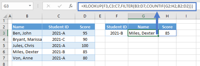
Let’s walk through the formula:
COUNTIF Function
First, let’s use the COUNTIF Function to count the instance of each source header (e.g., B2:D2) from the output headers (e.g., M2:N2).
=COUNTIF(M2:N2,B2:D2)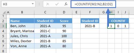
FILTER Function
The array result of the COUNTIF Function is then used as the filter condition to filter the columns.
=FILTER(B3:D7,H3:J3)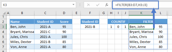
XLOOKUP Function
Finally, we can use the result of the FILTER Function in the XLOOKUP Function to return the columns that we want.
=XLOOKUP(F3,C3:C7,K3:L7)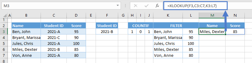
Combining all functions together yields our original formula:
=XLOOKUP(F3,C3:C7,FILTER(B3:D7,COUNTIF(G2:H2,B2:D2)))XLOOKUP-CHOOSE Return Columns in Different Order
The XLOOKUP-FILTER-COUNTIF Formula can return non-adjacent columns, but what if we want to return any column in a different order? To solve this, let’s use the CHOOSE Function.
=XLOOKUP(F3,B3:B7,CHOOSE({2,1},C3:C7,D3:D7))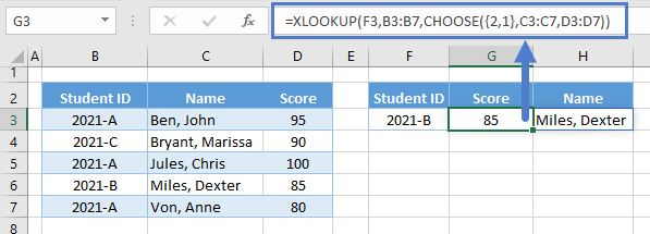
Let’s walk through the formula:
CHOOSE Function
First, we use the CHOOSE Function to join columns in a specified order into one array.
=CHOOSE({2,1},C3:C7,D3:D7)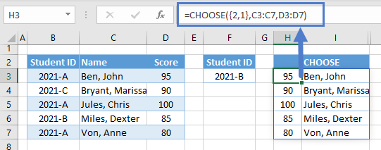
Note: We input the columns that we want separately in the CHOOSE Function (e.g., C3:C7, D3:D7), and we order them using the index_num (1st argument).
XLOOKUP Function
The resulting array from the CHOOSE Function is then used as the return array.
=XLOOKUP(F3,B3:B7,H3:I7)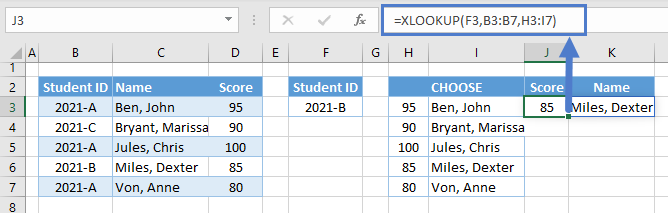
Combining all functions together yields our original formula:
=XLOOKUP(F3,B3:B7,CHOOSE({2,1},C3:C7,D3:D7))XLOOKUP-CHOOSECOLS Return Columns in Different Order
The XLOOKUP-CHOOSE Formula becomes long and tedious if we have a lot of columns to return. Luckily, there’s a new array function (currently in the BETA Version of Excel 365) that is more convenient than CHOOSE Function – CHOOSECOLS Function.
=XLOOKUP(F3,B3:B7,CHOOSECOLS(B3:D7,3,2))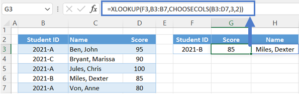
Let’s walk through the formula:
CHOOSECOLS Function
Unlike the CHOOSE Function where we join the columns in a specified order, the CHOOSECOLS Function returns the columns that we selected in the order that we specified.
=CHOOSECOLS(B3:D7,3,2)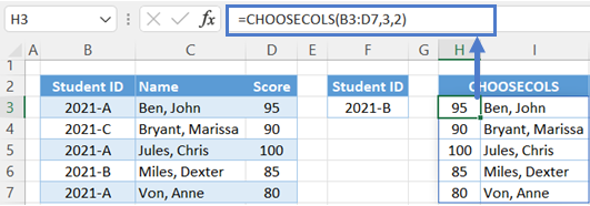
Note: The numbers that we specify in the col_num arguments (starting from the 2nd argument) are the relative column numbers of the columns from the given array (e.g., B3:D7).
XLOOKUP Function
Finally, we can use the XLOOKUP Function with the result of the CHOOSECOLS Function.
=XLOOKUP(F3,B3:B7,H3:I7)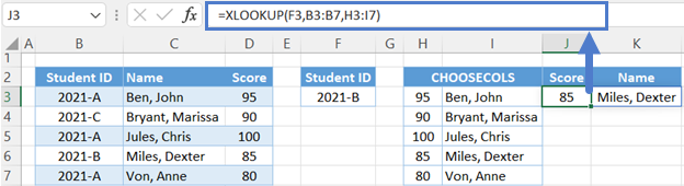
Combining all functions together yields our original formula:
=XLOOKUP(F3,B3:B7,CHOOSECOLS(B3:D7,3,2))XLOOKUP-CHOOSECOLS-MATCH Return Columns in Different Order
Instead of manually selecting the columns and their order, we can use the MATCH Function to automatically determine the columns and their order that are required by the task.
=XLOOKUP(F3,B3:B7,CHOOSECOLS(B3:D7,MATCH(G2:H2,B2:D2,0)))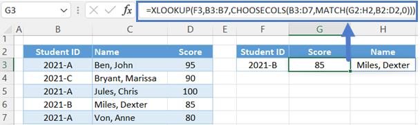
Let’s walk through the formula:
MATCH Function
First, we use the MATCH Function to determine the relative column positions of each output header from the source headers.
=MATCH(L2:M2,B2:D2,0)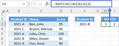
CHOOSECOLS Function
Now that we have the positions of the selected columns, we can use the CHOOSECOLS Function to return the selected columns in one array.
=CHOOSECOLS(B3:D7,H3:I3)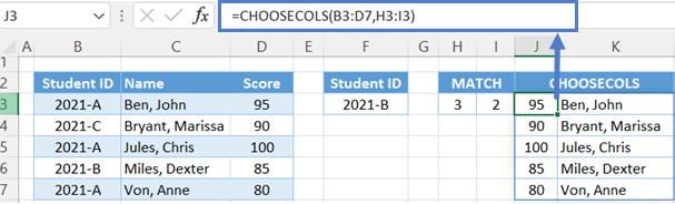
XLOOKUP Function
The last step is feeding the result of the CHOOSECOLS Function to the return array of the XLOOKUP Function.
=XLOOKUP(F3,B3:B7,J3:K7)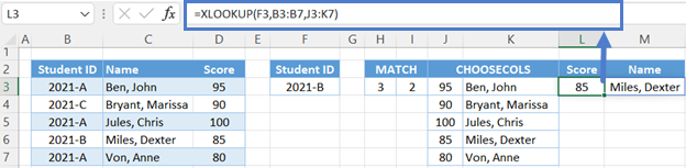
Combining all functions together yields our original formula:
=XLOOKUP(F3,B3:B7,CHOOSECOLS(B3:D7,MATCH(G2:H2,B2:D2,0)))
In this article, we will learn How to Only Return Results from Non-Blank Cells in Microsoft Excel.
What is a blank and non blank cell in Excel?
In Excel, Sometimes we don’t even want blank cells to disturb the formula. Most of the time we don’t want to work with a blank cell as it creates errors using the function. For Example VLOOKUP function returns #NA error when match type value is left blank. There are many functions like ISERROR which treats errors, but In this case we know the error is because of an empty value. So We learn the ISBLANK function in a formula with IF function.
IF — ISBLANK formula in Excel
ISBLANK function returns TRUE or FALSE boolean values based on the condition that the cell reference used is blank or not. Then use the required formula in the second or third argument.
Syntax of formula:
=IF(ISBLANK(cell_ref),[formula_if_blank],[ formula_if_false]
Cell ref : cell to check, if cell is blank or not.
Formula_if_true : formula or value if the cell is blank. Use Empty value («») if you want empty cell in return
Formula_if_false : formula or value if the cell is not blank. Use Empty value («») if you want empty cell in return
Example :
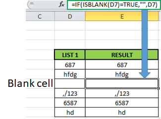
All of these might be confusing to understand. Let’s understand how to use the function using an example. Here we have some values on list 1 and we only want the formula to return the same value if not blank and empty value if blank.
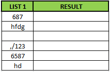
Formula:
=IF(ISBLANK(D5)=TRUE,«», D5)
Explanation:
ISBLANK : function checks the cell D5.
«» : returns an empty string blank cell instead of Zero.
IF function performs a logic_test if the test is true, it returns an empty string else returns the same value.
The resulting output will be like
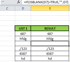
As you can see the formula returns the same value or blank cell based on the logic_test.
ISBLANK function with example
ISBLANK function returns TRUE or FALSE having cell reference as input.
Syntax:
Cell_ref : cell reference of cell to check e.g. B3
All of these might be confusing to understand. Let’s understand how to use the function using an example. Here We have some Values to test the function, except in the A5 cell. A5 cell has a formula that returns empty text.
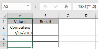
Use the Formula
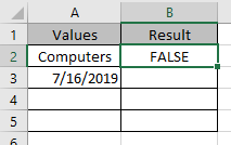
It returns False as there is text in the A2 cell.
Applying the formula in other cells using Ctrl + D shortcut key.
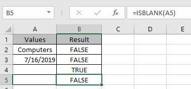
You must be wondering why didn’t the function returns False. As A5 cell has a formula making it non blank.
Hope this article about How to Only Return Results from Non-Blank Cells in Microsoft Excel is explanatory. Find more articles on blank values and related Excel formulas here. If you liked our blogs, share it with your friends on Facebook. And also you can follow us on Twitter and Facebook. We would love to hear from you, do let us know how we can improve, complement or innovate our work and make it better for you. Write to us at info@exceltip.com.
Related Articles :
Adjusting a Formula to Return a Blank : Formula adjusts its result on the basis of whether the cell is blank or not. Click the link to know how to use ISBLANK function with IF function in Excel.
Checking Whether Cells in a Range are Blank, and Counting the Blank Cells : If cells in a range are blank and calculating the blank cells in Excel then follow the link to understand more.
How to Calculate Only If Cell is Not Blank in Excel : Calculate only and only if the cell is not blank then use ISBLANK function in Excel.
Delete drop down list in Excel : The dropdown list is used to restrict the user to input data and gives the option to select from the list. We need to delete or remove the Dropdown list as the user will be able to input any data instead of choosing from a list.
Deleting All Cell Comments in Excel 2016 : Comments in Excel to remind ourselves and inform someone else about what the cell contains. To add the comment in a cell, Excel 2016 provides the insert Comment function. After inserting the comment it is displayed with little red triangles.
How to Delete only Filtered Rows without the Hidden Rows in Excel :Many of you are asking how to delete the selected rows without disturbing the other rows. We will use the Find & Select option in Excel.
How to Delete Sheets Without Confirmation Prompts Using VBA In Excel :There are times when we have to create or add sheets and later on we find no use of that sheet, hence we get the need to delete sheets quickly from the workbook
Popular Articles :
How to use the IF Function in Excel : The IF statement in Excel checks the condition and returns a specific value if the condition is TRUE or returns another specific value if FALSE.
How to use the VLOOKUP Function in Excel : This is one of the most used and popular functions of excel that is used to lookup value from different ranges and sheets.
How to use the SUMIF Function in Excel : This is another dashboard essential function. This helps you sum up values on specific conditions.
How to use the COUNTIF Function in Excel : Count values with conditions using this amazing function. You don’t need to filter your data to count specific values. Countif function is essential to prepare your dashboard.