
17 авг. 2022 г.
читать 2 мин
По умолчанию функция ВПР в Excel ищет некоторое значение в диапазоне и возвращает соответствующее значение только для первого совпадения .
Однако вы можете использовать следующий синтаксис для поиска некоторого значения в диапазоне и возврата соответствующих значений для всех совпадений :
=FILTER( C2:C11 , E2 = A2:A11 )
Эта конкретная формула просматривает диапазон C2:C11 и возвращает соответствующие значения в диапазоне A2:A11 для всех строк , где значение в C2:C11 равно E2 .
В следующем примере показано, как использовать этот синтаксис на практике.
Пример. Используйте функцию ВПР для возврата всех совпадений.
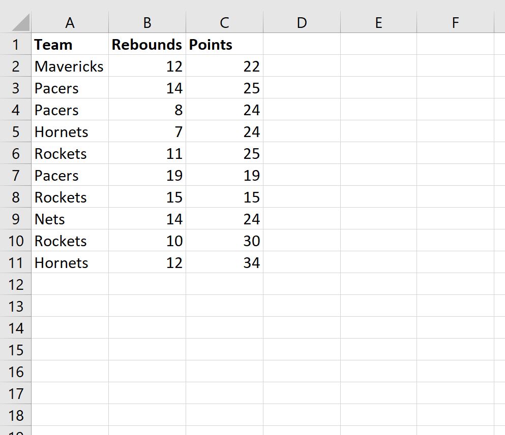
Предположим, у нас есть следующий набор данных в Excel, который показывает информацию о различных баскетбольных командах:
Предположим, мы используем следующую формулу с ВПР , чтобы найти команду «Ракеты» в столбце А и вернуть соответствующее значение очков в столбце С:
=VLOOKUP( E2 , A2:C11 , 3)
На следующем снимке экрана показано, как использовать эту формулу на практике:
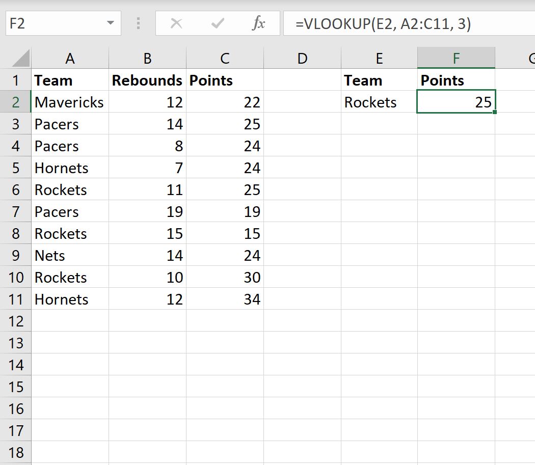
Функция ВПР возвращает значение в столбце «Очки» для первого появления слова «Ракеты» в столбце «Команда», но не возвращает значения очков для двух других строк, которые также содержат «Ракеты» в столбце «Команда».
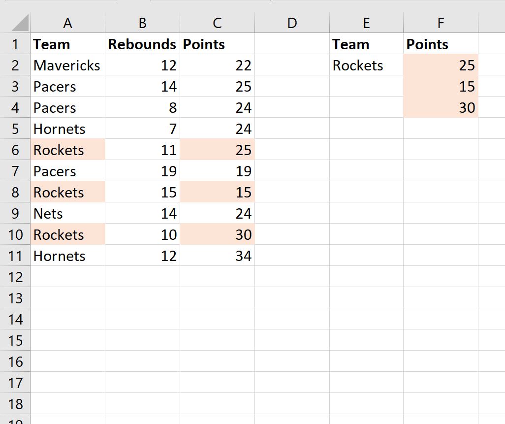
Чтобы вернуть значения очков для всех строк, содержащих ракеты в столбце «Команда», вместо этого мы можем использовать функцию ФИЛЬТР .
Вот точная формула, которую мы можем использовать:
=FILTER( C2:C11 , E2 = A2:A11 )
На следующем снимке экрана показано, как использовать эту формулу на практике:
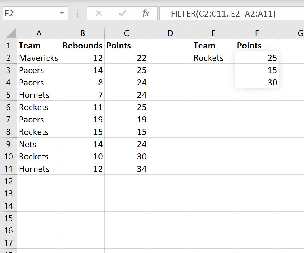
Обратите внимание, что функция ФИЛЬТР возвращает все три значения очков для трех строк, в которых столбец «Команда» содержит «Ракеты».
Связанный: Расширенный фильтр Excel: как использовать «Содержит»
Дополнительные ресурсы
В следующих руководствах объясняется, как выполнять другие распространенные операции в Excel:
Как сравнить два списка в Excel с помощью функции ВПР
Как найти уникальные значения из нескольких столбцов в Excel
Как отфильтровать несколько столбцов в Excel
By default, the VLOOKUP function in Excel looks up some value in a range and returns a corresponding value only for the first match.
However, you can use the following syntax to look up some value in a range and return corresponding values for all matches:
=FILTER(C2:C11, E2=A2:A11)
This particular formula looks in the range C2:C11 and returns the corresponding values in the range A2:A11 for all rows where the value in C2:C11 is equal to E2.
The following example shows how to use this syntax in practice.
Suppose we have the following dataset in Excel that shows information about various basketball teams:

Suppose we use the following formula with VLOOKUP to look up the team “Rockets” in column A and return the corresponding points value in column C:
=VLOOKUP(E2, A2:C11, 3)
The following screenshot shows how to use this formula in practice:

The VLOOKUP function returns the value in the “Points” column for the first occurrence of Rockets in the “Team” column, but it fails to return the points values for the other two rows that also contain Rockets in the “Team” column.
To return the points values for all rows that contain Rockets in the “Team” column, we can use the FILTER function instead.
Here’s the exact formula we can use:
=FILTER(C2:C11, E2=A2:A11)
The following screenshot shows how to use this formula in practice:

Notice that the FILTER function returns all three points values for the three rows where the “Team” column contains Rockets.

Related: Excel Advanced Filter: How to Use “Contains”
Additional Resources
The following tutorials explain how to perform other common operations in Excel:
How to Compare Two Lists in Excel Using VLOOKUP
How to Find Unique Values from Multiple Columns in Excel
How to Filter Multiple Columns in Excel
Method #1: INDEX and AGGREGATE
(Places all returned answers in separate cells)
Pros:
- Works with any version of Excel
- Does not require the use of CTRL-Shift-Enter to create an array formula
Cons:
- More complex than Method #2
Method #2: TEXTJOIN
(Places all returned answers in a single cell as a delimited list)
Pros:
- Simpler than Method #1
Cons:
- Requires Excel 2016 and Office 365
- Requires the use of CTRL-Shift-Enter to create an array formula
Objective: Have the user select a Division name and use the selected Division to return a list of associated Apps.
In our table, the selected Division names should return lists like the following:
| Utility | Productivity | Game |
|---|---|---|
| Accord | Blend | Fightrr |
| Misty Wash | Sleops | Hackrr |
| Twenty20 | WenCal | Kryptis |
| Perino |
Method #1 – INDEX and AGGREGATE
This method will use the INDEX function with the AGGREGATE function to locate the associated Apps for the selected Division and compile the results into a new list. We will also integrate an IF test to visually suppress any errors that may show up when the returned items do not fully populate the results list area.
To begin, select cell G4 and enter the Division “Game”.

NOTE: We could provide the user with a drop-down list to ease the selection process for Division, but for simplicity, we will hardcode the Division name. For a tutorial on creating unique dropdown lists from existing multi-valued lists, click the link below.
Excel: Extract unique items for dynamic data validation drop down list
The most common function people use when finding items in an Excel list is VLOOKUP. If you require a refresher on the use of VLOOKUP, click the link below.
Excel VLOOKUP: Basics of VLOOKUP and HLOOKUP explained with examples
The problem with using VLOOKUP in this scenario is that VLOOKUP will always stop on the first encountered matching item in the search list. If we are searching for “Game”, the VLOOKUP will always stop in cell A7.


We want to build a list where the 1st occurrence of a “Game” App is placed in cell G5; the 2nd occurrence is placed in cell G6; the 3rd in cell G7; etc.
We will use the INDEX and AGGREGATE functions to create this list. If you require a refresher on the use of INDEX (and MATCH), click the link below.
How to use Excel INDEX MATCH (the right way)
Select cell G5 and begin by creating an INDEX function.
=INDEX(array, row_num, [column_num])The INDEX function has the following parameters:
- Array = the cells to have items extracted from and returned as answers.
- Row_num = the “up and down” position in the list to move to extract data.
- Column_num = the “left to right” position in the list to move to extract data.
We want to extract App names from cells B5:B14.
=INDEX($B$5:$B$14We want to return the App named “Fightrr” from the 3rd position in the App list, so as a test we will hard-code the number “3”.
=INDEX($B$5:$B$14,3)If we fill the formula down the cells in column “G”, the App named “Fightrr” appears repeatedly, a behavior like the earlier VLOOKUP results. We need to find a way to have the row_num’s return value change from “3” to “4” to “5” to “7”. We cannot simply increase the value of the row-num parameter by 1 every time we repeat the formula; the parameter needs to change based on the position of the associated Division in column “A”.
We will use the AGGREGATE function to generate a list of rows (i.e. positions) where the selected Division (“Game”) is discovered. The advantage of using the AGGREGATE function is that it can accept multiple answers without the use of CTRL-Shift-Enter.
The AGGREGATE function has the following parameters:
- Function_num = a number corresponding to a function in the AGGREGATE list.

We will use the SMALL function (number 15).
- Options = a number corresponding to a behavior for handling errors, hidden data, and other AGGREGATE and SUBTOTAL functions when mixed with data.

We will use option #3 to ignore all other issues.
- Array = the values to be aggregated.
We will select cells A5:A14. - [k] = optional value when using selection functions, like SMALL or LARGE.
We will save this parameter for later.
TIP: To focus on one problem at a time, we will build the AGGREGATE function off to the side in column “H”. Once the AGGREGATE function is working to our satisfaction, we will fold the logic of AGGREGATE into the INDEX function.
Select cell H5 and enter the following formula:
=AGGREGATE(15,3,$A$5:$A$14)If we highlight the array parameter and press F9, we will see that the supplied array returns the words located in cells A5:A14.
![]()
Our objective is not to find the smallest word; we want to know which cells in the array match our selected Division. To do this, we will test each cell in the array to see if it matches the selected Division. Modify the array as follows.
=AGGREGATE(15,3,($A$5:$A$14=$G$4))If we highlight the array parameter and press F9, we will see the following test results.
![]()
The problem here is that Excel interprets a FALSE response as 0 (zero) and a TRUE response as 1 (one). If we use the SMALL function for discovery, the 0 will be selected first. We want to convert the FALSE responses to errors and the TRUE responses to position numbers within the list (i.e. 3, 4, 5, 7). To do this, we will divide the array by itself.
=AGGREGATE(15,3,(($A$5:$A$14=$G$4)/($A$5:$A$14=$G$4)))Because 0 ÷ 0 = ERROR and 1 ÷ 1 = 1, we get the following list of responses.
![]()
To change the 1’s to position numbers, we will multiply each 1 by its corresponding row number.
=AGGREGATE(15,3,(($A$5:$A$14=$G$4)/($A$5:$A$14=$G$4)*ROW($A$5:$A$14)))This will provide the following responses.
![]()
Because we didn’t start our list on row 1, our positions in the list are offset; in this case by 4 rows. Since the header for this table is in row 4, we will subtract the header row’s position value from the previous list of answers.
=AGGREGATE(15,3,(($A$5:$A$14=$G$4)/($A$5:$A$14=$G$4)*ROW($A$5:$A$14))-ROW($A$4))This will provide the following responses.
![]()
It’s now time to loop back and utilize the [k] option (the 4th parameter) of the AGGREGATE function. We want the SMALL function to increment by one for each copy of the AGGREGATE function. This will be accomplished by a cleaver trick of counting the cells in an ever-increasing range selection.
=AGGREGATE(15,3,(($A$5:$A$14=$G$4)/($A$5:$A$14=$G$4)*ROW($A$5:$A$14))-ROW($A$4),N)In this case, “N” will be the following function.
ROWS($F$5:F5)When used on the first AGGREGATE function, the result will be 1. By anchoring the beginning of the range to cell $F$5 as an absolute reference and leaving the ending of the range F5 as a relative reference, the range will change its size as the range ending moves further away from the range beginning.
| Cell | Function | Range Height (in cells) |
|---|---|---|
| H5 | ROWS($F$5:F5) | 1 |
| H6 | ROWS($F$5:F6) | 2 |
| H7 | ROWS($F$5:F7) | 3 |
| H8 | ROWS($F$5:F8) | 4 |
The formula with the intelligent row counter should appear as follows.
=AGGREGATE(15,3,(($A$5:$A$14=$G$4)/($A$5:$A$14=$G$4)*ROW($A$5:$A$14))-ROW($A$4), ROWS($F$5:F5))Now copy the formula (without the equals sign) from cell H5 and paste it into the row_num parameter of the INDEX function in cell G5. The updated formula should appear as follows.
Original formula
=INDEX($B$5:$B$14,3)Updated formula
=INDEX($B$5:$B$14,AGGREGATE(15,3,(($A$5:$A$14=$G$4)/($A$5:$A$14=$G$4)*ROW($A$5:$A$14))-ROW($A$4), ROWS($F$5:F5)))Fill the formula down through cells G5:G14. We now have the list of associated Apps to the selected Division as well as errors for when our return list is shorter than our expected maximum list length.

We want to hide the errors.
The simple (read “lazy”) way of hiding the errors is to nest the entire INDEX/AGGREGATE function in an IFERROR function like the following.
=IFERROR(INDEX($B$5:$B$14,AGGREGATE(15,3,(($A$5:$A$14=$G$4)/($A$5:$A$14=$G$4)*ROW($A$5:$A$14))-ROW($A$4), ROWS($F$5:F5))),””)The problem is that the IFERROR must fully process the INDEX/AGGREGATE function to determine if an error is generated. This can lead to many wasted CPU cycles when generating long lists of associated Apps.
The better tactic is to use an IF statement to count the number of times the selected Division appears in the list of Divisions and then compare that against the current App list’s length. If the App list length exceed the number of times the selected Division appears in the original Division list, the IF function will not execute the INDEX/AGGREGATE formula.
To give the IF function something to compare against, select cell F4 and enter the following “helper” formula.
=COUNTIF(A5:A14,G4)The updated IF function will perform the following test.
=IF(ROWS($F$5:F5)<=$F$4,INDEX/AGGREGATE,"")This formula will test the ever-expanding range that begins in cell F5 to determine if the range height exceeds the value supplied by the helper cell F4. The updated formula will appear as follows.
=IF(ROWS($F$5:F5)<=$F$4,INDEX($B$5:$B$14,AGGREGATE(15,3,(($A$5:$A$14=$G$4)/($A$5:$A$14=$G$4)*ROW($A$5:$A$14))-ROW($A$4), ROWS($F$5:F5))),"")Because “Game” has 4 entries in column “A”, when we get to the 5th iteration the ROWS function in the IF function will generate a 5. The test becomes “5<=4” which generates a FALSE condition, thereby display the empty text supplied by the two double quotes.
BONUS:
If you don’t want to have the “helper” formula in cell F4, you can fold the COUNTIF logic into the IF function. The updated formula would appear as follows.
=IF(ROWS($F$5:F5)<=COUNTIF($A$5:$A$15,$G$4),INDEX($B$5:$B$14,AGGREGATE(15,3,(($A$5:$A$14=$G$4)/($A$5:$A$14=$G$4)*ROW($A$5:$A$14))-ROW($A$4), ROWS($F$5:F5))),"")NOTE: When the COUNTIF was in a “helper” cell, we did not make any of the references absolute because we were not repeating the formula across any other cells. If we fold the COUNTIF logic into the IF function, we need to make the references absolute due to the repeated nature of the formula in column “G”.
The only drawback to this consolidation is that the counting of the selected Division must be repeated for each IF function. In longer lists (i.e. hundreds of thousands of rows), this could negatively impact processing time. By performing the COUNTIF as a separate “helper” calculation, it must only be performed once.
Method #2 – TEXTJOIN
Using the TEXTJOIN function (available in Excel 2016 of Office 365) we will perform
The TEXTJOIN function has the following parameters:
- Delimiter – the character that separates the returned values.
We will create a comma-delimited list, so we will enter “,”. - Ignore_empty – This determines whether to include any empty cells in the results list.
We are unsure as to our needs, so we will use FALSE and change it later if needed. - Text1 – This is the range of cells containing the source data.
We will select A5:A14.
Begin by selecting cell G4 and replacing the Division “Game” with “Utility”.
Select cell H5 and entering in the following formula.
=TEXTJOIN(“,”,False,B5:B14)This provides the following result.
Accord,Blend,Fightrr,Hackrr,Kryptis,Misty Wash,Perino,Sleops,Twenty20,WenCaLWe do not want the complete list of Apps, we only want Apps that are associated with the selected Division (cell G4). To filter the list to only associated Apps, we will perform a logical test, using IF, to compare each of the Apps’ associated Division with the selected Division. Update the formula as follows. Remember to finish the formula by pressing CTRL-Shift-Enter.
=TEXTJOIN(",",FALSE,IF(A5:A14=G4,B5:B14,""))This provides the following result.
Accord,,,,,Misty Wash,,,Twenty20,If we highlight the IF function in the formula and press F9 we will see the following responses.
![]()
To remove the empty cell notations, update the formula by changing the Ignore_empty parameter from FALSE to TRUE. Remember to finish the formula by pressing CTRL-Shift-Enter.
=TEXTJOIN(",",TRUE,IF(A5:A14=G4,B5:B14,""))This provides the following result.
Accord,Misty Wash,Twenty20Feel free to Download the Workbook HERE.
![]()
Published on: August 30, 2018
Last modified: March 9, 2023


Leila Gharani
I’m a 5x Microsoft MVP with over 15 years of experience implementing and professionals on Management Information Systems of different sizes and nature.
My background is Masters in Economics, Economist, Consultant, Oracle HFM Accounting Systems Expert, SAP BW Project Manager. My passion is teaching, experimenting and sharing. I am also addicted to learning and enjoy taking online courses on a variety of topics.
In this Excel XLookup Return All Matches Tutorial, you learn how to create an Excel XLookup return all matches formula.
The Excel XLookup return all matches formula template/structure you learn below relies on the FILTER function. FILTER is available in Excel 2021 and later (including Excel 365).
This Excel XLookup Return All Matches Tutorial is accompanied by an Excel workbook with the data and formulas I use. Get this example workbook (for free) by clicking the button below.

Related Excel Training Materials and Resources
The following Excel VLookup Tutorials may help you better understand the differences between the XLOOKUP and VLOOKUP functions (XLOOKUP vs. VLOOKUP).
- Excel VLOOKUP Tutorial (under development): Click here to open.
- Excel VLOOKUP from Another Sheet: Click here to open.
- Excel VLOOKUP Compare 2 Columns and Find Matches: Click here to open.
- Excel VLookup Sum Multiple Row Values (in Same Column): Click here to open.
- Excel VLOOKUP Multiple Columns: Click here to open.
- Excel VLOOKUP Sum Multiple Columns (Values): Click here to open.
- Excel VLookup Sum Multiple Column Values (with XLOOKUP): Click here to open.
- Excel VLookup Sum Multiple Rows and Columns: Click here to open.
- Excel VLookup Multiple Criteria with INDEX MATCH: Click here to open.
- Excel VLookup Multiple Criteria with XLOOKUP: Click here to open.
- Excel VLookup Multiple Criteria with the FILTER Function: Click here to open.
- Excel VLOOKUP Return Multiple Values with Helper Column: Click here to open.
- Excel VLookup Return Multiple Values with the INDEX Function: Click here to open.
- Excel VLookup Return Multiple Values with the FILTER Function: Click here to open.
- Excel VLookup Return Multiple Values in One Cell Separated by a Comma: Click here to open.
- Excel VLOOKUP Multiple Sheets: Click here to open.
- Excel VLOOKUP Multiple Sheets in Different Workbook: Click here to open.
- Excel VLOOKUP Sheet in Multiple Different Workbooks: Click here to open.
This Excel XLookup Return All Matches Tutorial is part of a more comprehensive series of Excel XLOOKUP Tutorials.
- Excel XLOOKUP Tutorial: Click here to open.
- Excel XLOOKUP in Table: Click here to open.
- Excel Nested XLOOKUP (Dynamic Lookup Value): Click here to open.
- Excel XLOOKUP If Not Found Return Blank: Click here to open.
- Excel IF XLOOKUP (for Error Handling): Click here to open.
- Excel XLOOKUP If Blank Return Blank: Click here to open.
- Excel XLOOKUP Wildcard: Click here to open.
- Excel XLOOKUP Between 2 Values: Click here to open.
- Excel XLookup Return All Matches: Click here to open.
You can find more Excel and VBA Tutorials in the organized Tutorials Archive: Click here to visit the Archives. The following are some of my most popular Excel Tutorials and Training Resources:
- Excel Keyboard Shortcuts Cheat Sheet: Click here to open.
- Excel Power Query (Get & Transform) Tutorial for Beginners: Click here to open.
- Excel Macro Tutorial for Beginners: Click here to open.
If you want to learn more about Excel essentials, Excel formulas, and similar Excel topics, you may be interested in taking one (or more) Excel Courses: Click here to learn more about these Excel Courses (affiliate link).
If you want to learn how to automate Excel (and save time) by working with macros and VBA, you may be interested in the following Premium Excel Macro and VBA Training Materials:
- Premium Courses at the Power Spreadsheets Academy: Click here to open.
- Books at the Power Spreadsheets Library: Click here to open.
If you need help with Excel tasks/projects, you may be interested in working with me: Click here to learn more about working with me.
Excel XLookup Return All Matches Formula Template/Structure
'Source: https://powerspreadsheets.com/
'More information: https://powerspreadsheets.com/excel-xlookup-all-matches/
=FILTER(ColumnOrRowWithValuesToReturn,ColumnOrRowWhereYouSearch=LookupValue)
Step-by-Step Process to Create an Excel XLookup Return All Matches Formula
(1) Call the FILTER function.
'Source: https://powerspreadsheets.com/
'More information: https://powerspreadsheets.com/excel-xlookup-all-matches/
=FILTER(...)
(2) Use the first argument of the FILTER function (array) to specify the return array. This is the column (when doing a VLookup) or row (when doing an HLookup) with the value to return.
'Source: https://powerspreadsheets.com/
'More information: https://powerspreadsheets.com/excel-xlookup-all-matches/
=FILTER(ColumnOrRowWithValuesToReturn,...)
(3) Set the second argument of the FILTER function (include) to an expression with the following 3 items:
- The column (when doing a VLookup) or row (when doing an HLookup) where you search for the lookup value (the lookup array).
- The equal to comparison operator (=).
- The value you search for in the column (when doing a VLookup) or row (when doing an HLookup) you search in (the lookup value).
Ensure the number of rows (when doing a VLookup) or columns (when doing an HLookup) of the lookup array (you specify in this step #3) is the same as that of the return array (you specified in step #2).
'Source: https://powerspreadsheets.com/
'More information: https://powerspreadsheets.com/excel-xlookup-all-matches/
=FILTER(ColumnOrRowWithValuesToReturn,ColumnOrRowWhereYouSearch=LookupValue)
How (and Why) the XLookup Return All Matches Formula Works
The XLOOKUP function:
- Searches a range or array for a match; and
- Returns the corresponding item(s) from a second range or array.
XLOOKUP returns the item(s) corresponding to a single (the first) match.
You can (however) work with the FILTER function to return all matches (create an Excel XLookup return all matches formula). The FILTER function:
- Filters an array based on the criteria (for example, a lookup value) you specify; and
- Returns an array with all applicable (filtered) matches.
This Excel XLookup Return All Matches Tutorial is accompanied by an Excel workbook with the data and formulas I use. Get this example workbook (for free) by clicking the button below.
Excel XLookup Return All Matches Example Worksheet
The example worksheet has 3 tables/sections with the following characteristics:
(1) Table 1 (cells A6 to H26).
The table:
- With the data.
- Where I search with the XLookup return all matches example formula.
(2) Lookup value (cells J6 and K6).
The lookup value (Salesperson  is stored in cell K6.
(3) XLookup return all matches example formula (cells J8 to K13).
- Cell J9 stores the XLookup return all matches example formula.
- Cells J9 to J13 display the results. This is because:
- The array returned by the XLookup return all matches example formula has 5 items; and
- Results spill from cell J9 into cells J10 to J13.
- Cell K9 displays the XLookup return all matches example formula I enter in cell J9.

Excel XLookup Return All Matches Example Formula
The XLookup return all matches example formula stored in cell J9 is as follows:
'Source: https://powerspreadsheets.com/
'More information: https://powerspreadsheets.com/excel-xlookup-all-matches/
=FILTER(H7:H26,A7:A26=K6)
The lookup value (stored in cell K6) is “Salesperson 8”.
This value is found in the following rows of the column I search in with the XLookup return all matches example formula (column A, cells A7 to A26):
- Row 8 (cell A8).
- Row 12 (cell A12).
- Row 17 (cell A17).
- Row 22 (cell A22).
- Row 25 (cell A25).

Download the Excel XLookup Return All Matches Example Workbook
This Excel XLookup Return All Matches Tutorial is accompanied by an Excel workbook with the data and formulas I use. Get this example workbook (for free) by clicking the button below.
Related Excel Training Materials and Resources
The following Excel VLookup Tutorials may help you better understand the differences between the XLOOKUP and VLOOKUP functions (XLOOKUP vs. VLOOKUP).
- Excel VLOOKUP Tutorial (under development): Click here to open.
- Excel VLOOKUP from Another Sheet: Click here to open.
- Excel VLOOKUP Compare 2 Columns and Find Matches: Click here to open.
- Excel VLookup Sum Multiple Row Values (in Same Column): Click here to open.
- Excel VLOOKUP Multiple Columns: Click here to open.
- Excel VLOOKUP Sum Multiple Columns (Values): Click here to open.
- Excel VLookup Sum Multiple Column Values (with XLOOKUP): Click here to open.
- Excel VLookup Sum Multiple Rows and Columns: Click here to open.
- Excel VLookup Multiple Criteria with INDEX MATCH: Click here to open.
- Excel VLookup Multiple Criteria with XLOOKUP: Click here to open.
- Excel VLookup Multiple Criteria with the FILTER Function: Click here to open.
- Excel VLOOKUP Return Multiple Values with Helper Column: Click here to open.
- Excel VLookup Return Multiple Values with the INDEX Function: Click here to open.
- Excel VLookup Return Multiple Values with the FILTER Function: Click here to open.
- Excel VLookup Return Multiple Values in One Cell Separated by a Comma: Click here to open.
- Excel VLOOKUP Multiple Sheets: Click here to open.
- Excel VLOOKUP Multiple Sheets in Different Workbook: Click here to open.
- Excel VLOOKUP Sheet in Multiple Different Workbooks: Click here to open.
This Excel XLookup Return All Matches Tutorial is part of a more comprehensive series of Excel XLOOKUP Tutorials.
- Excel XLOOKUP Tutorial: Click here to open.
- Excel XLOOKUP in Table: Click here to open.
- Excel Nested XLOOKUP (Dynamic Lookup Value): Click here to open.
- Excel XLOOKUP If Not Found Return Blank: Click here to open.
- Excel IF XLOOKUP (for Error Handling): Click here to open.
- Excel XLOOKUP If Blank Return Blank: Click here to open.
- Excel XLOOKUP Wildcard: Click here to open.
- Excel XLOOKUP Between 2 Values: Click here to open.
- Excel XLookup Return All Matches: Click here to open.
You can find more Excel and VBA Tutorials in the organized Tutorials Archive: Click here to visit the Archives. The following are some of my most popular Excel Tutorials and Training Resources:
- Excel Keyboard Shortcuts Cheat Sheet: Click here to open.
- Excel Power Query (Get & Transform) Tutorial for Beginners: Click here to open.
- Excel Macro Tutorial for Beginners: Click here to open.
If you want to learn more about Excel essentials, Excel formulas, and similar Excel topics, you may be interested in taking one (or more) Excel Courses: Click here to learn more about these Excel Courses (affiliate link).
If you want to learn how to automate Excel (and save time) by working with macros and VBA, you may be interested in the following Premium Excel Macro and VBA Training Materials:
- Premium Courses at the Power Spreadsheets Academy: Click here to open.
- Books at the Power Spreadsheets Library: Click here to open.
If you need help with Excel tasks/projects, you may be interested in working with me: Click here to learn more about working with me.
I created named ranges for COLOR and PROD_ID to make this more readable:
=IF(VLOOKUP(COLOR,IF(A1:A6=PROD_ID,B1:C6,»»),2,0),1,0)
Hit CTRL+SHIFT+ENTER when you enter this formula, it is an array formula, and will not work if don’t enter it that way. I will explain it from the inside out (as well as I can, because I do not full understand part of it. This is assuming data is in cells A1:C6 (no headers).
Entering as an array function allows the inner IF to cycle through A1:A6=PROD_ID, for every match, it adds a tuple to a temporary array, so after the inner loop completes, it returns the array {«Green», 0; «Blue», 1; «»,»»; «»,»»; «»,»»; «»,»»; } — in a more readable format, this is (please forgive my horrible «more readable» format):
—Col1—|—Col2
-«Green»-|—0
—«Blue»—|—1
—«»——-|—«»
—«»——-|—«»
—«»——-|—«»
—«»——-|—«»
Your vlookup then runs against this, returning 1 (row 2) to the outer-most if. Unfortunately, I’m a bit fuzzy on how the bolded part of my formula works, I just know it will return the appropriate row in that range as needed.
Note: in more recent versions of Excel, the FILTER function is a better way to solve this problem. The INDEX and MATCH formula explained here is meant for legacy versions of Excel that do not provide the FILTER function.
By default, lookup formulas in Excel like VLOOKUP and INDEX + MATCH will find the first match, but not other matches that may exist in a set of data. However, with some effort, you can make INDEX and MATCH return all matches. One way to approach this problem is to use a helper column to return a numeric value that indicates a match. This makes it much easier to identify and extract multiple matches.
Helper column
A helper column is a way to simplify a complex formula in Excel by breaking the problem down into smaller steps. In the worksheet shown, a helper column is used to identify matching data based on conditions entered in the range I3:J3. The formula in the helper column in cell E3 looks like this:
=SUM(E2,AND(C3=$I$3,D3=$J$3))
The helper column tests each row in the data to see if the Department in column C matches the value in I3 and the Building in column D matches the value in J3. Both logical tests must return TRUE in order for AND to return TRUE.
For each row, the result from the AND function is added to the «value above» in the helper column to generate a count. The practical effect of this formula is an incrementing counter that only changes when a (new) match is found. Then the value remains the same until the next match is found. This works because the TRUE/FALSE results return by AND are coerced to 1/0 values as part of the sum operation. FALSE results add nothing and TRUE results add 1.
Back in the extraction area, the lookup formula for Name in column H looks like this:
=IF($G6<=ct,INDEX(data,MATCH($G6,helper,0),1),"")
Working from the inside out, the INDEX + MATCH part of the formula looks up the name for the first match found, using the row number in column G as the match value:
INDEX(data,MATCH($G6,helper,0),1)
INDEX receives all 3 columns of data as the array (named range «data»), and MATCH is configured to match the row number inside the helper column (the named range «helper») in exact match mode (3rd argument set to zero).
This is where the cleverness of the formula becomes apparent. The helper column obviously contains duplicates, but it doesn’t matter, because MATCH will match only the first value. By design, each «first value» corresponds to the correct row in the data table.
The formulas in columns I and J are the same as H, except for the column number, which is increased in each case by one.
The IF statement that wraps the INDEX/MATCH formula performs a simple function — it checks each row number in the extraction area to see if the row number is less than or equal to the value in G3 (named range «ct»), which is the total count of all matching records. If so, the INDEX/MATCH logic is run. If not, IF outputs an empty string («»).
The formula in G3 (named range «ct») is simple:
=MAX(helper)
Since the maximum value in the helper column is the same as the total match count, the MAX function is all we need.
Note: the extraction area needs to be manually configured to handle as much data as needed (i.e. 5 rows, 10 rows, 20 rows, etc.). In this example, it is limited to 5 rows only to keep the worksheet compact.
I learned this technique in Mike Girvin’s book Control + Shift + Enter.
The FILTER function
If you have a current version of Excel, the FILTER function is a better way to extract all matching records.
XLOOKUP can’t return all matches by default; however, here is the workaround with the Excel FILTER function.
If we are talking about lookup functions in Excel, everyone knows that XLOOKUP is a swiss-knife in Excel. Good to know that it works the same as other lookups; it returns the first matching record corresponding to a lookup value. The good news is that there is a workaround with the FILTER function. Take a closer look at the example and read the step-by-step guide. If you want to learn all about XLOOKUP, check our definitive guide.
General Formula to get all matching values using the FILTER function:
=FILTER(return array, lookup array = lookup value)- Enter the FILTER function
- Define the first argument, return_array
- Use an expression as the second argument: lookup_array = lookup_value
- The formula returns all matching records
Explanation, Syntax, and Arguments
This section will show you how the formula works through a simple example. Before deeply diving into the details, take a closer look at the FILTER function syntax and arguments.
Syntax:
=FILTER(array, include, [if_empty])The FILTER function uses two required and one optional argument to get all matches:
Arguments:
- array: the array that contains the possible matches
- include: filters an array based on the criteria
- [if_empty] – optional argument: error-handling option in case of no match found
First, create two named ranges to simplify the formula. Select the range, locate the name box and enter a descriptive name for a given range.
- data: range B3:G12
- totals: range G3:12
Enter the following formula in cell I5:
=FILTER(data, totals=281)The second argument, [include], will find and extract all matching records from the “data” range.
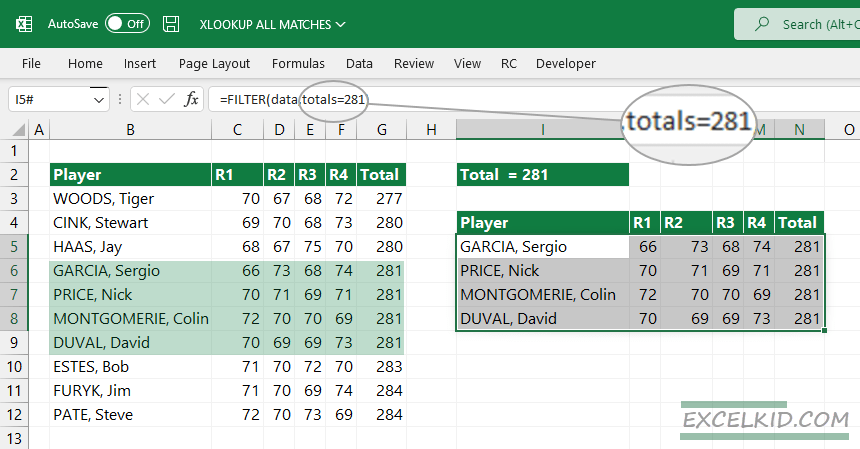
You can use the FILTER function to filter data based on custom criteria. In the example, we want to return the matching rows where the total score equals 281. The formula returns multiple results, and Excel will (like other dynamic array functions in Excel) spill all records that meet the criteria.
Download the practice file (.zip)
Additional resources:
- Learn all about the FILTER function
- Find the 2nd match using XLOOKUP

Istvan is the co-founder of Visual Analytics Ltd. He writes blog posts and helps people to reach the top in Excel.
MATCH function
Tip: Try using the new XMATCH function, an improved version of MATCH that works in any direction and returns exact matches by default, making it easier and more convenient to use than its predecessor.
The MATCH function searches for a specified item in a range of cells, and then returns the relative position of that item in the range. For example, if the range A1:A3 contains the values 5, 25, and 38, then the formula =MATCH(25,A1:A3,0) returns the number 2, because 25 is the second item in the range.

Tip: Use MATCH instead of one of the LOOKUP functions when you need the position of an item in a range instead of the item itself. For example, you might use the MATCH function to provide a value for the row_num argument of the INDEX function.
Syntax
MATCH(lookup_value, lookup_array, [match_type])
The MATCH function syntax has the following arguments:
-
lookup_value Required. The value that you want to match in lookup_array. For example, when you look up someone’s number in a telephone book, you are using the person’s name as the lookup value, but the telephone number is the value you want.
The lookup_value argument can be a value (number, text, or logical value) or a cell reference to a number, text, or logical value.
-
lookup_array Required. The range of cells being searched.
-
match_type Optional. The number -1, 0, or 1. The match_type argument specifies how Excel matches lookup_value with values in lookup_array. The default value for this argument is 1.
The following table describes how the function finds values based on the setting of the match_type argument.
|
Match_type |
Behavior |
|
1 or omitted |
MATCH finds the largest value that is less than or equal to lookup_value. The values in the lookup_array argument must be placed in ascending order, for example: …-2, -1, 0, 1, 2, …, A-Z, FALSE, TRUE. |
|
0 |
MATCH finds the first value that is exactly equal to lookup_value. The values in the lookup_array argument can be in any order. |
|
-1 |
MATCH finds the smallest value that is greater than or equal tolookup_value. The values in the lookup_array argument must be placed in descending order, for example: TRUE, FALSE, Z-A, …2, 1, 0, -1, -2, …, and so on. |
-
MATCH returns the position of the matched value within lookup_array, not the value itself. For example, MATCH(«b»,{«a»,»b»,»c«},0) returns 2, which is the relative position of «b» within the array {«a»,»b»,»c»}.
-
MATCH does not distinguish between uppercase and lowercase letters when matching text values.
-
If MATCH is unsuccessful in finding a match, it returns the #N/A error value.
-
If match_type is 0 and lookup_value is a text string, you can use the wildcard characters — the question mark (?) and asterisk (*) — in the lookup_value argument. A question mark matches any single character; an asterisk matches any sequence of characters. If you want to find an actual question mark or asterisk, type a tilde (~) before the character.
Example
Copy the example data in the following table, and paste it in cell A1 of a new Excel worksheet. For formulas to show results, select them, press F2, and then press Enter. If you need to, you can adjust the column widths to see all the data.
|
Product |
Count |
|
|
Bananas |
25 |
|
|
Oranges |
38 |
|
|
Apples |
40 |
|
|
Pears |
41 |
|
|
Formula |
Description |
Result |
|
=MATCH(39,B2:B5,1) |
Because there is not an exact match, the position of the next lowest value (38) in the range B2:B5 is returned. |
2 |
|
=MATCH(41,B2:B5,0) |
The position of the value 41 in the range B2:B5. |
4 |
|
=MATCH(40,B2:B5,-1) |
Returns an error because the values in the range B2:B5 are not in descending order. |
#N/A |
Need more help?
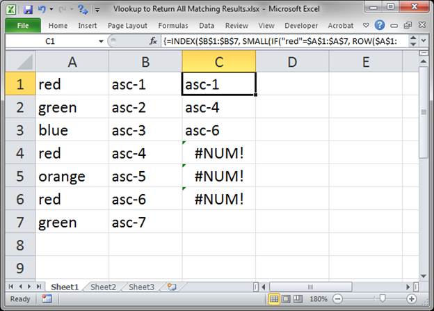
Here is an Excel formula that will act like a Vlookup that returns every matching result from a list.
Note: all formulas below are array formulas and so must be entered using Ctrl + Shift + Enter.
Sections:
The Formula
Formula That Hides Errors
Notes
The Formula
=INDEX($B$1:$B$7, SMALL(IF($A$1=$A$1:$A$7, ROW($A$1:$A$7)-ROW($A$1)+1), ROW(1:1)))
This is an Array Formula and so you must enter it into the cell using Ctrl + Shift + Enter.
This is a confusing formula so let me break it down for you.
First, there is no Vlookup function in there; the title of the tutorial says Vlookup because that is what most people understand, instead of «Index Array Formula to Return all Results.»
What to Change to Work for Your Example
$A$1:$A$7 is the range reference that contains the values that you search through. You will need to change this in two locations within the formula.
$B$1:$B$7 is the range reference of the data that you want to return. This should be the same shape and size as the first range reference above.
ROW($A$1) contains the range reference of the very first cell in the data set through which you will search.
$A$1=$A$1:$A$7 the $A$1 part of this section contains the cell that you will use to lookup data. You can keep this as a cell reference or you can hard-code a text or number value in here. For text, wrap it with double quotation marks like this: «red» but for numbers you do not need to put quotation marks around it. In this example, it is the first cell in the lookup column, but it could be any cell within the worksheet or workbook, it doesn’t matter where it is.
Here is an example of the code where this part is hardcoded for the text «red»:
=INDEX($B$1:$B$7, SMALL(IF(«red»=$A$1:$A$7, ROW($A$1:$A$7)-ROW($A$1)+1), ROW(1:1)))
ROW(1:1) should always be this for the first formula and it should be left as a relative cell reference (without dollar signs). This is important because this is what tells the formula which value in the list to return. When you copy the entire formula down, the number should increment by 1; ROW(1:1), ROW(2:2), ROW(3:3), etc. So, if you have three results for the text «red» this part of the formula says to return result 1, result 2, result 3, etc. Basically, leave this part alone and you should be OK.
Copy the formula down: you will enter this formula into the first cell and make sure that it works like it should. Then select that cell and copy it down as far as you need to return all of the results in the list.
Here is what is looks like in Excel:
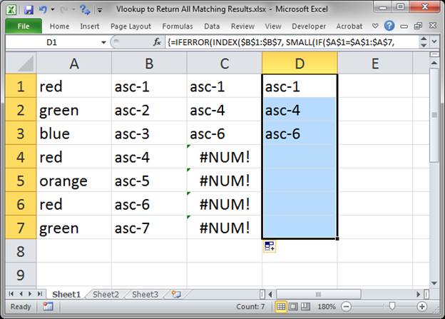
Formula That Hides Errors
This formula has nice output instead of the ugly #NUM! error when a result isn’t found.
This is the same base formula as above and so the details of that formula will not be covered again. The formula here is simply put within an error checking function.
Excel 2007+
=IFERROR(INDEX($B$1:$B$7, SMALL(IF($A$1=$A$1:$A$7, ROW($A$1:$A$7)-ROW($A$1)+1), ROW(1:1))),"")
In Excel 2007 and later we can use the IFERROR function to output a blank when there are no more results to return. This has the benefit of making it look like the list just appears as needed.
Excel 2003
=IF(ISERROR(INDEX($B$1:$B$7, SMALL(IF($A$1=$A$1:$A$7, ROW($A$1:$A$7)-ROW($A$1)+1), ROW(1:1)))),"",INDEX($B$1:$B$7, SMALL(IF($A$1=$A$1:$A$7, ROW($A$1:$A$7)-ROW($A$1)+1), ROW(1:1))))
This is for Excel versions prior to Excel 2007, such as Excel 2003.
This uses the same base formula as above except we have to use the IF function combined with the ISERROR function (there is no IFERROR() function in Excel 2003).
This looks confusing because it’s quite long but it’s really just the same base formula written twice. The ISERROR function checks if the formula creates an error or not and, if it does, it outputs a blank, but, if it works, then it moves to the second part of the IF statement, which contains the formula that we want to use.
It’s a bit confusing, but this is how you have to hide errors for Excel 2003 and earlier.
Notes
This is a complex formula that involves a lot of moving parts; just remember that you don’t have to understand every part of the formula in order to use it correctly, just edit the above formula, as specified, to fit your dataset.
Make sure to download the sample file to get these formulas in Excel.
Similar Content on TeachExcel
Vlookup Macro to Return All Matching Results from a Sheet in Excel
Macro: This Excel Macro works like a better Vlookup function because it returns ALL of the matchi…
Vlookup Macro to Return All Matching Results and Stack them with Previous Results
Macro: This is very similar to the other Vlookup type Macro in that it returns all of the results…
How to Quickly Find Data Anywhere in Excel
Tutorial:
Finding specific records and/or cells is easy when using the Find tool in Excel. It is lo…
Vlookup Date Picker in Excel (Dynamic)
Tutorial: Make a dynamically updating vlookup date picker for excel that allows you to choose a date…
Excel 365 Wildcard Vlookup to Return All Partial Matches
Tutorial: This post is related to the following video:
TeachExcel explained how to perform a Vlooku…
Vlookup to Return the Min, Max, or Average Value in Excel
Tutorial:
Perform a Vlookup that returns the highest value, lowest value, or average value from a d…