
Overview of formulas in Excel
Get started on how to create formulas and use built-in functions to perform calculations and solve problems.

Important: The calculated results of formulas and some Excel worksheet functions may differ slightly between a Windows PC using x86 or x86-64 architecture and a Windows RT PC using ARM architecture. Learn more about the differences.
Important: In this article we discuss XLOOKUP and VLOOKUP, which are similar. Try using the new XLOOKUP function, an improved version of VLOOKUP that works in any direction and returns exact matches by default, making it easier and more convenient to use than its predecessor.
Create a formula that refers to values in other cells
-
Select a cell.
-
Type the equal sign =.
Note: Formulas in Excel always begin with the equal sign.
-
Select a cell or type its address in the selected cell.

-
Enter an operator. For example, – for subtraction.
-
Select the next cell, or type its address in the selected cell.
-
Press Enter. The result of the calculation appears in the cell with the formula.


See a formula
-
When a formula is entered into a cell, it also appears in the Formula bar.
-
To see a formula, select a cell, and it will appear in the formula bar.


Enter a formula that contains a built-in function
-
Select an empty cell.
-
Type an equal sign = and then type a function. For example, =SUM for getting the total sales.
-
Type an opening parenthesis (.
-
Select the range of cells, and then type a closing parenthesis).
-
Press Enter to get the result.

Download our Formulas tutorial workbook
We’ve put together a Get started with Formulas workbook that you can download. If you’re new to Excel, or even if you have some experience with it, you can walk through Excel’s most common formulas in this tour. With real-world examples and helpful visuals, you’ll be able to Sum, Count, Average, and Vlookup like a pro.
Formulas in-depth
You can browse through the individual sections below to learn more about specific formula elements.
A formula can also contain any or all of the following: functions, references, operators, and constants.
Parts of a formula

1. Functions: The PI() function returns the value of pi: 3.142…
2. References: A2 returns the value in cell A2.
3. Constants: Numbers or text values entered directly into a formula, such as 2.
4. Operators: The ^ (caret) operator raises a number to a power, and the * (asterisk) operator multiplies numbers.
A constant is a value that is not calculated; it always stays the same. For example, the date 10/9/2008, the number 210, and the text «Quarterly Earnings» are all constants. An expression or a value resulting from an expression is not a constant. If you use constants in a formula instead of references to cells (for example, =30+70+110), the result changes only if you modify the formula. In general, it’s best to place constants in individual cells where they can be easily changed if needed, then reference those cells in formulas.
A reference identifies a cell or a range of cells on a worksheet, and tells Excel where to look for the values or data you want to use in a formula. You can use references to use data contained in different parts of a worksheet in one formula or use the value from one cell in several formulas. You can also refer to cells on other sheets in the same workbook, and to other workbooks. References to cells in other workbooks are called links or external references.
-
The A1 reference style
By default, Excel uses the A1 reference style, which refers to columns with letters (A through XFD, for a total of 16,384 columns) and refers to rows with numbers (1 through 1,048,576). These letters and numbers are called row and column headings. To refer to a cell, enter the column letter followed by the row number. For example, B2 refers to the cell at the intersection of column B and row 2.
To refer to
Use
The cell in column A and row 10
A10
The range of cells in column A and rows 10 through 20
A10:A20
The range of cells in row 15 and columns B through E
B15:E15
All cells in row 5
5:5
All cells in rows 5 through 10
5:10
All cells in column H
H:H
All cells in columns H through J
H:J
The range of cells in columns A through E and rows 10 through 20
A10:E20
-
Making a reference to a cell or a range of cells on another worksheet in the same workbook
In the following example, the AVERAGE function calculates the average value for the range B1:B10 on the worksheet named Marketing in the same workbook.
1. Refers to the worksheet named Marketing
2. Refers to the range of cells from B1 to B10
3. The exclamation point (!) Separates the worksheet reference from the cell range reference
Note: If the referenced worksheet has spaces or numbers in it, then you need to add apostrophes (‘) before and after the worksheet name, like =’123′!A1 or =’January Revenue’!A1.
-
The difference between absolute, relative and mixed references
-
Relative references A relative cell reference in a formula, such as A1, is based on the relative position of the cell that contains the formula and the cell the reference refers to. If the position of the cell that contains the formula changes, the reference is changed. If you copy or fill the formula across rows or down columns, the reference automatically adjusts. By default, new formulas use relative references. For example, if you copy or fill a relative reference in cell B2 to cell B3, it automatically adjusts from =A1 to =A2.
Copied formula with relative reference
-
Absolute references An absolute cell reference in a formula, such as $A$1, always refer to a cell in a specific location. If the position of the cell that contains the formula changes, the absolute reference remains the same. If you copy or fill the formula across rows or down columns, the absolute reference does not adjust. By default, new formulas use relative references, so you may need to switch them to absolute references. For example, if you copy or fill an absolute reference in cell B2 to cell B3, it stays the same in both cells: =$A$1.
Copied formula with absolute reference
-
Mixed references A mixed reference has either an absolute column and relative row, or absolute row and relative column. An absolute column reference takes the form $A1, $B1, and so on. An absolute row reference takes the form A$1, B$1, and so on. If the position of the cell that contains the formula changes, the relative reference is changed, and the absolute reference does not change. If you copy or fill the formula across rows or down columns, the relative reference automatically adjusts, and the absolute reference does not adjust. For example, if you copy or fill a mixed reference from cell A2 to B3, it adjusts from =A$1 to =B$1.
Copied formula with mixed reference
-
-
The 3-D reference style
Conveniently referencing multiple worksheets If you want to analyze data in the same cell or range of cells on multiple worksheets within a workbook, use a 3-D reference. A 3-D reference includes the cell or range reference, preceded by a range of worksheet names. Excel uses any worksheets stored between the starting and ending names of the reference. For example, =SUM(Sheet2:Sheet13!B5) adds all the values contained in cell B5 on all the worksheets between and including Sheet 2 and Sheet 13.
-
You can use 3-D references to refer to cells on other sheets, to define names, and to create formulas by using the following functions: SUM, AVERAGE, AVERAGEA, COUNT, COUNTA, MAX, MAXA, MIN, MINA, PRODUCT, STDEV.P, STDEV.S, STDEVA, STDEVPA, VAR.P, VAR.S, VARA, and VARPA.
-
3-D references cannot be used in array formulas.
-
3-D references cannot be used with the intersection operator (a single space) or in formulas that use implicit intersection.
What occurs when you move, copy, insert, or delete worksheets The following examples explain what happens when you move, copy, insert, or delete worksheets that are included in a 3-D reference. The examples use the formula =SUM(Sheet2:Sheet6!A2:A5) to add cells A2 through A5 on worksheets 2 through 6.
-
Insert or copy If you insert or copy sheets between Sheet2 and Sheet6 (the endpoints in this example), Excel includes all values in cells A2 through A5 from the added sheets in the calculations.
-
Delete If you delete sheets between Sheet2 and Sheet6, Excel removes their values from the calculation.
-
Move If you move sheets from between Sheet2 and Sheet6 to a location outside the referenced sheet range, Excel removes their values from the calculation.
-
Move an endpoint If you move Sheet2 or Sheet6 to another location in the same workbook, Excel adjusts the calculation to accommodate the new range of sheets between them.
-
Delete an endpoint If you delete Sheet2 or Sheet6, Excel adjusts the calculation to accommodate the range of sheets between them.
-
-
The R1C1 reference style
You can also use a reference style where both the rows and the columns on the worksheet are numbered. The R1C1 reference style is useful for computing row and column positions in macros. In the R1C1 style, Excel indicates the location of a cell with an «R» followed by a row number and a «C» followed by a column number.
Reference
Meaning
R[-2]C
A relative reference to the cell two rows up and in the same column
R[2]C[2]
A relative reference to the cell two rows down and two columns to the right
R2C2
An absolute reference to the cell in the second row and in the second column
R[-1]
A relative reference to the entire row above the active cell
R
An absolute reference to the current row
When you record a macro, Excel records some commands by using the R1C1 reference style. For example, if you record a command, such as clicking the AutoSum button to insert a formula that adds a range of cells, Excel records the formula by using R1C1 style, not A1 style, references.
You can turn the R1C1 reference style on or off by setting or clearing the R1C1 reference style check box under the Working with formulas section in the Formulas category of the Options dialog box. To display this dialog box, click the File tab.
Top of Page


Need more help?
You can always ask an expert in the Excel Tech Community or get support in the Answers community.
See Also
Switch between relative, absolute and mixed references for functions
Using calculation operators in Excel formulas
The order in which Excel performs operations in formulas
Using functions and nested functions in Excel formulas
Define and use names in formulas
Guidelines and examples of array formulas
Delete or remove a formula
How to avoid broken formulas
Find and correct errors in formulas
Excel keyboard shortcuts and function keys
Excel functions (by category)
Need more help?
Formulas and functions are the bread and butter of Excel. They drive almost everything interesting and useful you will ever do in a spreadsheet. This article introduces the basic concepts you need to know to be proficient with formulas in Excel. More examples here.
What is a formula?
A formula in Excel is an expression that returns a specific result. For example:
=1+2 // returns 3

=6/3 // returns 2

Note: all formulas in Excel must begin with an equals sign (=).
Cell references
In the examples above, values are «hardcoded». That means results won’t change unless you edit the formula again and change a value manually. Generally, this is considered bad form, because it hides information and makes it harder to maintain a spreadsheet.
Instead, use cell references so values can be changed at any time. In the screen below, C1 contains the following formula:
=A1+A2+A3 // returns 9

Notice because we are using cell references for A1, A2, and A3, these values can be changed at any time and C1 will still show an accurate result.
All formulas return a result
All formulas in Excel return a result, even when the result is an error. Below a formula is used to calculate percent change. The formula returns a correct result in D2 and D3, but returns a #DIV/0! error in D4, because B4 is empty:

There are different ways of handling errors. In this case, you could provide the missing value in B4, or «catch» the error with the IFERROR function and display a more friendly message (or nothing at all).
Copy and paste formulas
The beauty of cell references is that they automatically update when a formula is copied to a new location. This means you don’t need to enter the same basic formula again and again. In the screen below, the formula in E1 has been copied to the clipboard with Control + C:

Below: formula pasted to cell E2 with Control + V. Notice cell references have changed:

Same formula pasted to E3. Cell addresses are updated again:

Relative and absolute references
The cell references above are called relative references. This means the reference is relative to the cell it lives in. The formula in E1 above is:
=B1+C1+D1 // formula in E1
Literally, this means «cell 3 columns left «+ «cell 2 columns left» + «cell 1 column left». That’s why, when the formula is copied down to cell E2, it continues to work in the same way.
Relative references are extremely useful, but there are times when you don’t want a cell reference to change. A cell reference that won’t change when copied is called an absolute reference. To make a reference absolute, use the dollar symbol ($):
=A1 // relative reference
=$A$1 // absolute reference
For example, in the screen below, we want to multiply each value in column D by 10, which is entered in A1. By using an absolute reference for A1, we «lock» that reference so it won’t change when the formula is copied to E2 and E3:

Here are the final formulas in E1, E2, and E3:
=D1*$A$1 // formula in E1
=D2*$A$1 // formula in E2
=D3*$A$1 // formula in E3
Notice the reference to D1 updates when the formula is copied, but the reference to A1 never changes. Now we can easily change the value in A1, and all three formulas recalculate. Below the value in A1 has changed from 10 to 12:

This simple example also shows why it doesn’t make sense to hardcode values into a formula. By storing the value in A1 in one place, and referring to A1 with an absolute reference, the value can be changed at any time and all associated formulas will update instantly.
Tip: you can toggle between relative and absolute syntax with the F4 key.
How to enter a formula
To enter a formula:
- Select a cell
- Enter an equals sign (=)
- Type the formula, and press enter.
Instead of typing cell references, you can point and click, as seen below. Note references are color-coded:

All formulas in Excel must begin with an equals sign (=). No equals sign, no formula:

How to change a formula
To edit a formula, you have 3 options:
- Select the cell, edit in the formula bar
- Double-click the cell, edit directly
- Select the cell, press F2, edit directly
No matter which option you use, press Enter to confirm changes when done. If you want to cancel, and leave the formula unchanged, click the Escape key.
Video: 20 tips for entering formulas
What is a function?
Working in Excel, you will hear the words «formula» and «function» used frequently, sometimes interchangeably. They are closely related, but not exactly the same. Technically, a formula is any expression that begins with an equals sign (=).
A function, on the other hand, is a formula with a special name and purpose. In most cases, functions have names that reflect their intended use. For example, you probably know the SUM function already, which returns the sum of given references:
=SUM(1,2,3) // returns 6
=SUM(A1:A3) // returns A1+A2+A3
The AVERAGE function, as you would expect, returns the average of given references:
=AVERAGE(1,2,3) // returns 2
And the MIN and MAX functions return minimum and maximum values, respectively:
=MIN(1,2,3) // returns 1
=MAX(1,2,3) // returns 3
Excel contains hundreds of specific functions. To get started, see 101 Key Excel functions.
Function arguments
Most functions require inputs to return a result. These inputs are called «arguments». A function’s arguments appear after the function name, inside parentheses, separated by commas. All functions require a matching opening and closing parentheses (). The pattern looks like this:
=FUNCTIONNAME(argument1,argument2,argument3)
For example, the COUNTIF function counts cells that meet criteria, and takes two arguments, range and criteria:
=COUNTIF(range,criteria) // two arguments
In the screen below, range is A1:A5 and criteria is «red». The formula in C1 is:
=COUNTIF(A1:A5,"red") // returns 2

Video: How to use the COUNTIF function
Not all arguments are required. Arguments shown in square brackets are optional. For example, the YEARFRAC function returns fractional number of years between a start date and end date and takes 3 arguments:
=YEARFRAC(start_date,end_date,[basis])
Start_date and end_date are required arguments, basis is an optional argument. See below for an example of how to use YEARFRAC to calculate current age based on birthdate.
How to enter a function
If you know the name of the function, just start typing. Here are the steps:
1. Enter equals sign (=) and start typing. Excel will make a list of matching functions based as you type:

When you see the function you want in the list, use the arrow keys to select (or just keep typing).
2. Type the Tab key to accept a function. Excel will complete the function:

3. Fill in required arguments:

4. Press Enter to confirm formula:

Combining functions (nesting)
Many Excel formulas use more than one function, and functions can be «nested» inside each other. For example, below we have a birthdate in B1 and we want to calculate current age in B2:

The YEARFRAC function will calculate years with a start date and end date:

We can use B1 for start date, then use the TODAY function to supply the end date:

When we press Enter to confirm, we get current age based on today’s date:
=YEARFRAC(B1,TODAY())

Notice we are using the TODAY function to feed an end date to the YEARFRAC function. In other words, the TODAY function can be nested inside the YEARFRAC function to provide the end date argument. We can take the formula one step further and use the INT function to chop off the decimal value:
=INT(YEARFRAC(B1,TODAY()))

Here, the original YEARFRAC formula returns 20.4 to the INT function, and the INT function returns a final result of 20.
Notes:
- The current date in images above is February 22, 2019.
- Nested IF functions are a classic example of nesting functions.
- The TODAY function is a rare Excel function with no required arguments.
Key takeaway: The output of any formula or function can be fed directly into another formula or function.
Math Operators
The table below shows the standard math operators available in Excel:
| Symbol | Operation | Example |
|---|---|---|
| + | Addition | =2+3=5 |
| — | Subtraction | =9-2=7 |
| * | Multiplication | =6*7=42 |
| / | Division | =9/3=3 |
| ^ | Exponentiation | =4^2=16 |
| () | Parentheses | =(2+4)/3=2 |
Logical operators
Logical operators provide support for comparisons such as «greater than», «less than», etc. The logical operators available in Excel are shown in the table below:
| Operator | Meaning | Example |
|---|---|---|
| = | Equal to | =A1=10 |
| <> | Not equal to | =A1<>10 |
| > | Greater than | =A1>100 |
| < | Less than | =A1<100 |
| >= | Greater than or equal to | =A1>=75 |
| <= | Less than or equal to | =A1<=0 |
Video: How to build logical formulas
Order of operations
When solving a formula, Excel follows a sequence called «order of operations». First, any expressions in parentheses are evaluated. Next Excel will solve for any exponents. After exponents, Excel will perform multiplication and division, then addition and subtraction. If the formula involves concatenation, this will happen after standard math operations. Finally, Excel will evaluate logical operators, if present.
- Parentheses
- Exponents
- Multiplication and Division
- Addition and Subtraction
- Concatenation
- Logical operators
Tip: you can use the Evaluate feature to watch Excel solve formulas step-by-step.
Convert formulas to values
Sometimes you want to get rid of formulas, and leave only values in their place. The easiest way to do this in Excel is to copy the formula, then paste, using Paste Special > Values. This overwrites the formulas with the values they return. You can use a keyboard shortcut for pasting values, or use the Paste menu on the Home tab on the ribbon.
Video: Paste Special Shortcuts
What’s next?
Below are guides to help you learn more about Excel’s formulas and functions. We also offer online video training.
- 29 tips for working with formulas and functions (video version here)
- 500 formula examples with full explanations
- 101 important Excel functions
- Guide to all Excel functions (work in progress)
- Excel formula errors (examples and fixes)
- Formula criteria — 50 examples
- Formulas for conditional formatting
- How to use F9 to debug a formula (video)
- Excel formula errors and fixes (video)
Suppose I have a function attached to one of my Excel sheets:
Public Function foo(bar As Integer) as integer
    foo = 42
End Function
How can I get the results of foo returned to a cell on my sheet? I’ve tried "=foo(10)", but all it gives me is "#NAME?"
I’ve also tried =[filename]!foo(10) and [sheetname]!foo(10) with no change.
![]()
asked Feb 17, 2009 at 21:46
![]()
Try following the directions here to make sure you’re doing everything correctly, specifically about where to put it. ( Insert->Module )
I can confirm that opening up the VBA editor, using Insert->Module, and the following code:
Function TimesTwo(Value As Integer)
    TimesTwo = Value * 2
End Function
and on a sheet putting "=TimesTwo(100)" into a cell gives me 200.
![]()
BIBD
15k25 gold badges85 silver badges137 bronze badges
answered Feb 17, 2009 at 22:11
![]()
StephenStephen
4,0762 gold badges24 silver badges29 bronze badges
0
Put the function in a new, separate module (Insert->Module), then use =foo(10) within a cell formula to invoke it.
answered Feb 17, 2009 at 21:53
![]()
anormanorm
2,2471 gold badge19 silver badges38 bronze badges
1
Where did you put the «foo» function? I don’t know why, but whenever I’ve seen this, the solution is to record a dimple macro, and let Excel create a new module for that macro’s code. Then, put your «foo» function in that module. Your code works when I follow this procedure, but if I put it in the code module attached to «ThisWorkbook,» I get the #NAME result you report.
answered Feb 17, 2009 at 22:22
![]()
JeffKJeffK
3,0192 gold badges26 silver badges29 bronze badges
include the file name like this
=PERSONAL.XLS!foo(10)
answered Feb 17, 2009 at 21:50
![]()
chilltempchilltemp
8,8068 gold badges41 silver badges46 bronze badges
1
Skip to content
В решении многих задач обычные функции Excel не всегда могут помочь. Если существующих функций недостаточно, Excel позволяет добавить новые настраиваемые пользовательские функции (UDF). Они делают вашу работу легче.
Мы расскажем, как можно их создать, какие они бывают и как использовать их, чтобы ваша работа стала проще. Узнайте, как записать и использовать пользовательские функции, которые многие называют макросами..
- Что такое пользовательская функция
- Для чего ее используют?
- Как создать пользовательскую функцию в VBA?
- Как использовать пользовательскую функцию в формуле?
- Какие бывают типы пользовательских функций
Что такое пользовательская функция в Excel?
На момент написания этой статьи Excel предлагает вам более 450 различных функций. С их помощью вы можете выполнять множество различных операций. Но разработчики Microsoft Excel не могли предвидеть все задачи, которые нам нужно решать. Думаю, что многие из вас встречались с этими проблемами:
- не все данные могут быть обработаны стандартными функциями (например, даты до 1900 года).
- формулы могут быть весьма длинными и сложными. Их невозможно запомнить, трудно понять и сложно изменить для решения новой задачи.
- Не все задачи могут быть решены при помощи стандартных функций Excel (в частности, нельзя извлечь интернет-адрес из гиперссылки).
- Невозможно автоматизировать часто повторяющиеся стандартные операции (импорт данных из бухгалтерской программы на лист Excel, форматирование дат и чисел, удаление лишних колонок).
Как можно решить эти проблемы?
- Для очень сложных формул многие пользователи создают архив рабочих книг с примерами. Они копируют оттуда нужную формулу и применяют ее в своей таблице.
- Создание макросов VBA.
- Создание пользовательских функций при помощи редактора VBA.
Хотя первые два варианта кажутся вам знакомыми, третий может вызвать некоторую путаницу. Итак, давайте подробнее рассмотрим настраиваемые функции в Excel и решим, стоит ли их использовать.
Пользовательская функция – это настраиваемый код, который принимает исходные данные, производит вычисление и возвращает желаемый результат.
Исходными данными могут быть числа, текст, даты, логические значения, массивы. Результатом вычислений может быть значение любого типа, с которым работает Excel, или массив таких значений.
Другими словами, пользовательская функция – это своего рода модернизация стандартных функций Excel. Вы можете использовать ее, когда возможностей обычных функций недостаточно. Основное ее назначение – дополнить и расширить возможности Excel, выполнить действия, которые невозможны со стандартными возможностями.
Существует несколько способов создания собственных функций:
- при помощи Visual Basic for Applications (VBA). Этот способ описывается в данной статье.
- с использованием замечательной функции LAMBDA, которая появилась в Office365.
- при помощи Office Scripts. На момент написания этой статьи они доступны в Excel Online в подписке на Office365.
Посмотрите на скриншот ниже, чтобы увидеть разницу между двумя способами извлечения чисел — с использованием формулы и пользовательской функции ExtractNumber().

Даже если вы сохранили эту огромную формулу в своем архиве, вам нужно ее найти, скопировать и вставить, а затем аккуратно поправить все ссылки на ячейки. Согласитесь, это потребует затрат времени, да и ошибки не исключены.
А на ввод функции вы потратите всего несколько секунд.
Для чего можно использовать?
Вы можете использовать настраиваемую функцию одним из следующих способов:
- В формуле, где она может брать исходные данные из вашего рабочего листа и возвращать рассчитанное значение или массив значений.
- Как часть кода макроса VBA или другой пользовательской функции.
- В формулах условного форматирования.
- Для хранения констант и списков данных.
Для чего нельзя использовать пользовательские функции:
- Любого изменения другой ячейки, кроме той, в которую она записана,
- Изменения имени рабочего листа,
- Копирования листов рабочей книги,
- Поиска и замены значений,
- Изменения форматирования ячейки, шрифта, фона, границ, включения и отключения линий сетки,
- Вызова и выполнения макроса VBA, если его выполнение нарушит перечисленные выше ограничения. Если вы используете строку кода, который не может быть выполнен, вы можете получить ошибку RUNTIME ERROR либо просто одну из стандартных ошибок (например, #ЗНАЧЕН!).
Как создать пользовательскую функцию в VBA?
Прежде всего, необходимо открыть редактор Visual Basic (сокращенно — VBE). Обратите внимание, что он открывается в новом окне. Окно Excel при этом не закрывается.
Самый простой способ открыть VBE — использовать комбинацию клавиш. Это быстро и всегда доступно. Нет необходимости настраивать ленту или панель инструментов быстрого доступа. Нажмите Alt + F11 на клавиатуре, чтобы открыть VBE. И снова нажмите Alt + F11, когда редактор открыт, чтобы вернуться назад в окно Excel.

После открытия VBE вам нужно добавить новый модуль. В него вы будете записывать ваш код. Щелкните правой кнопкой мыши на панели проекта VBA слева и выберите «Insert», затем появившемся справа окне — “Module”.
Справа появится пустое окно модуля, в котором вы и будете создавать свою функцию.
Прежде чем начать, напомним правила, по которым создается функция.
- Пользовательская функция всегда начинается с оператора Function и заканчивается инструкцией End Function.
- После оператора Function указывают имя функции. Это название, которое вы создаете и присваиваете, чтобы вы могли идентифицировать и использовать ее позже. Оно не должно содержать пробелов. Если вы хотите разделять слова, используйте подчеркивания. Например, Count_Words.
- Кроме того, это имя также не может совпадать с именами стандартных функций Excel. Если вы сделаете это, то всегда будет выполняться стандартная функция.
- Имя пользовательской функции не может совпадать с адресами ячеек на листе. Например, имя ABC1234 невозможно присвоить.
- Настоятельно рекомендуется давать описательные имена. Тогда вы можете легко выбрать нужное из длинного списка функций. Например, имя CountWords позволяет легко понять, что она делает, и при необходимости применить ее для подсчета слов.
- Далее в скобках обычно перечисляют аргументы. Это те данные, с которыми она будет работать. Может быть один или несколько аргументов. Если у вас несколько аргументов, их нужно перечислить через запятую.
- После этого обычно объявляются переменные, которые использует пользовательская функция. Указывается тип этих переменных – число, дата, текст, массив.
- Если операторы, которые вы используете внутри вашей функции, не используют никакие аргументы (например, NOW (СЕЙЧАС), TODAY (СЕГОДНЯ) или RAND (СЛЧИС)), то вы можете создать функцию без аргументов. Также аргументы не нужны, если вы используете функцию для хранения констант (например, числа Пи).
- Затем записывают несколько операторов VBA, которые выполняют вычисления с использованием переданных аргументов.
- В конце вы должны вставить оператор, который присваивает итоговое значение переменной с тем же именем, что и имя функции. Это значение возвращается в формулу, из которой была вызвана пользовательская функция.
- Записанный вами код может включать комментарии. Они помогут вам не забыть назначение функции и отдельных ее операторов. Если вы в будущем захотите внести какие-то изменения, комментарии будут вам очень полезны. Комментарий всегда начинается с апострофа (‘). Апостроф указывает Excel игнорировать всё, что записано после него, и до конца строки.
Теперь давайте попробуем создать вашу первую собственную формулу. Для начала мы создаем код, который будет подсчитывать количество слов в диапазоне ячеек.
Для этого в окно модуля вставим этот код:
Function CountWords(NumRange As Range) As Long
Dim rCell As Range, lCount As Long
    For Each rCell In NumRange
        lCount = lCount + _
          Len(WorksheetFunction.Trim(rCell)) - Len(Replace(WorksheetFunction.Trim(rCell), " ", "")) + 1
    Next rCell
CountWords = lCount
End Function
Я думаю, здесь могут потребоваться некоторые пояснения.
Код функции всегда начинается с пользовательской процедуры Function. В процедуре Function мы делаем описание новой функции.
В начале мы должны записать ее имя: CountWords.
Затем в скобках указываем, какие исходные данные она будет использовать. NumRange As Range означает, что аргументом будет диапазон значений. Сюда нужно передать только один аргумент — диапазон ячеек, в котором будет происходить подсчёт.
As Long указывает, что результат выполнения функции CountWords будет целым числом.
Во второй строке кода мы объявляем переменные.
Оператор Dim объявляет переменные:
rCell — переменная диапазона ячеек, в котором мы будем подсчитывать слова.
lCount — переменная целое число, в которой будет записано число слов.
Цикл For Each… Next предназначен для выполнения вычислений по отношению к каждому элементу из группы элементов (нашего диапазона ячеек). Этот оператор цикла применяется, когда неизвестно количество элементов в группе. Начинаем с первого элемента, затем берем следующий и так повторяем до самого последнего значения. Цикл повторяется столько раз, сколько ячеек имеется во входном диапазоне.
Внутри этого цикла с значением каждой ячейки выполняется операция, которая вычисляет количество слов:
Len(WorksheetFunction.Trim(rCell)) — Len(Replace(WorksheetFunction.Trim(rCell), » «, «»)) + 1
Как видите, это обычная формула Excel, которая использует стандартные средства работы с текстом: LEN, TRIM и REPLACE. Это английские названия знакомых нам русскоязычных ДЛСТР, СЖПРОБЕЛЫ и ЗАМЕНИТЬ. Вместо адреса ячейки рабочего листа используем переменную диапазона rCell. То есть, для каждой ячейки диапазона мы последовательно считаем количество слов в ней.
Подсчитанные числа суммируются и сохраняются в переменной lCount:
lCount = lCount + Len(WorksheetFunction.Trim(rCell)) — Len(Replace(WorksheetFunction.Trim(rCell), » «, «»)) + 1
Когда цикл будет завершен, значение переменной присваивается функции.
CountWords = lCount
Функция возвращает в ячейку рабочего листа значение этой переменной, то есть общее количество слов.
Именно эта строка кода гарантирует, что функция вернет значение lCount обратно в ячейку, из которой она была вызвана.
Закрываем наш код с помощью «End Function».
Как видите, не очень сложно.
Сохраните вашу работу. Для этого просто нажмите кнопку “Save” на ленте VB редактора.
После этого вы можете закрыть окно редактора. Для этого можно использовать комбинацию клавиш Alt+Q. Или просто вернитесь на лист Excel, нажав Alt+F11.
Вы можете сравнить работу с пользовательской функцией CountWords и подсчет количества слов в диапазоне при помощи формул.
Как использовать пользовательскую функцию в формуле?
Когда вы создали пользовательскую, она становится доступной так же, как и другие стандартные функции Excel. Сейчас мы узнаем, как создавать с ее помощью собственные формулы.
Чтобы использовать ее, у вас есть две возможности.
Первый способ. Нажмите кнопку fx в строке формул. Среди появившихся категорий вы увидите новую группу — Определённые пользователем. И внутри этой категории вы можете увидеть нашу новую пользовательскую функцию CountWords.

Второй способ. Вы можете просто записать эту функцию в ячейку так же, как вы это делаете обычно. Когда вы начинаете вводить имя, Excel покажет вам имя пользовательской в списке соответствующих функций. В приведенном ниже примере, когда я ввел = cou , Excel показал мне список подходящих функций, среди которых вы видите и CountWords.

Можно посчитать этой же функцией и количество слов в диапазоне. Запишите в ячейку С3:
=CountWords(A2:A5)
Нажмите Enter.
Мы только что указали функцию и установили диапазон, и вот результат подсчета: 14 слов.
Для сравнения в C1 я записал формулу массива, при помощи которой мы также можем подсчитать количество слов в диапазоне.

Как видите, результаты одинаковы. Только использовать CountWords() гораздо проще и быстрее.
Различные типы пользовательских функций с использованием VBA.
Теперь мы познакомимся с разными типами пользовательских функций в зависимости от используемых ими аргументов и результатов, которые они возвращают.
Без аргументов.
В Excel есть несколько стандартных функций, которые не требуют аргументов (например, СЛЧИС , СЕГОДНЯ , СЕЧАС). Например, СЛЧИС возвращает случайное число от 0 до 1. СЕГОДНЯ вернет текущую дату. Вам не нужно передавать им какие-либо значения.
Вы можете создать такую функцию и в VBA.
Ниже приведен код, который запишет в ячейку имя вашего рабочего листа.
Function SheetName() as String
    Application.Volatile
    SheetName = Application.Caller.Worksheet.Name
End Function
Или же можно использовать такой код:
SheetName = ActiveSheet.NameОбратите внимание, что в скобках после имени нет ни одного аргумента. Здесь не требуется никаких аргументов, так как результат, который нужно вернуть, не зависит от каких-либо значений в вашем рабочем файле.
Приведенный выше код определяет результат функции как тип данных String (поскольку желаемый результат — это имя файла, которое является текстом). Если вы не укажете тип данных, то Excel будет определять его самостоятельно.
С одним аргументом.
Создадим простую функцию, которая работает с одним аргументом, то есть с одной ячейкой. Наша задача – извлечь из текстовой строки последнее слово.
Function ReturnLastWord(The_Text As String)
Dim stLastWord As String
'Extracts the LAST word from a text string
    stLastWord = StrReverse(The_Text)
    stLastWord = Left(stLastWord, InStr(1, stLastWord, " ", vbTextCompare))
    ReturnLastWord = StrReverse(Trim(stLastWord))
End Function
Аргумент The_Text — это значение выбранной ячейки. Указываем, что это должно быть текстовое значение (As String).
Оператор StrReverse возвращает текст с обратным порядком следования знаков. Далее InStr определяет позицию первого пробела. При помощи Left получаем все знаки заканчивая первым пробелом. Затем удаляем пробелы при помощи Trim. Вновь меняем порядок следования символов при помощи StrReverse. Получаем последнее слово из текста.
Поскольку эта функция принимает значение ячейки, нам не нужно использовать здесь Application.Volatile. Как только аргумент изменится, функция автоматически обновится.
Использование массива в качестве аргумента.
Многие функции Excel используют массивы значений как аргументы. Вспомните функции СУММ, СУММЕСЛИ, СУММПРОИЗВ.
Мы уже рассмотрели эту ситуацию выше, когда учились создавать пользовательскую функцию для подсчета количества слов в диапазоне ячеек.
Приведённый ниже код создает функцию, которая суммирует все чётные числа в указанном диапазоне ячеек.
Function SumEven(NumRange as Range)
 Dim RngCell As Range
 For Each RngCell In NumRange
 If IsNumeric(RngCell.Value) Then
 If RngCell.Value Mod 2 = 0 Then
 Result = Result + RngCell.Value
 End If
 End If
 Next RngCell
 SumEven = Result
 End Function
Аргумент NumRange указан как Range. Это означает, что функция будет использовать массив исходных данных. Необходимо отметить, что можно использовать также тип переменной Variant. Это выглядит как
Function SumEven(NumRange as Variant)Тип Variant обеспечивает «безразмерный» контейнер для хранения данных. Такая переменная может хранить данные любого из допустимых в VBA типов, включая числовые значения, текст, даты и массивы. Более того, одна и та же такая переменная в одной и той же программе в разные моменты может хранить данные различных типов. Excel самостоятельно будет определять, какие данные передаются в функцию.
В коде есть цикл For Each … Next, который берет каждую ячейку и проверяет, есть ли в ней число. Если это не так, то ничего не происходит, и он переходит к следующей ячейке. Если найдено число, он проверяет, четное оно или нет (с помощью функции MOD).
Все чётные числа суммируются в переменной Result.
Когда цикл будет закончен, значение Result присваивается переменной SumEven и передаётся функции.
С несколькими аргументами.
Большинство функций Excel имеет несколько аргументов. Не являются исключением и пользовательские функции. Поэтому так важно уметь создавать собственные функции с несколькими аргументами.
В приведенном ниже коде создается функция, которая выбирает максимальное число в заданном интервале.
Она имеет 3 аргумента: диапазон значений, нижняя граница числового интервала, верхняя граница интервала.
Function GetMaxBetween(rngCells As Range, MinNum, MaxNum)
Dim NumRange As Range
Dim vMax
Dim arrNums()
Dim i As Integer
ReDim arrNums(rngCells.Count)
    For Each NumRange In rngCells
     vMax = NumRange
        Select Case vMax
           Case MinNum + 0.01 To MaxNum - 0.01
              arrNums(i) = vMax
              i = i + 1
           Case Else
               GetMaxBetween = 0
           End Select
    Next NumRange
    GetMaxBetween = WorksheetFunction.Max(arrNums)
End Function
Здесь мы используем три аргумента. Первый из них — rngCells As Range. Это диапазон ячеек, в которых нужно искать максимальное значение. Второй и третий аргумент (MinNum, MaxNum) указаны без объявления типа. Это означает, что по умолчанию к ним будет применён тип данных Variant. В VBA используется 6 различных числовых типов данных. Указывать только один из них — это значит ограничить применение функции. Поэтому более целесообразно, если Excel сам определит тип числовых данных.
Цикл For Each … Next последовательно просматривает все значения в выбранном диапазоне. Числа, которые находятся в интервале от максимального до минимального значения, записываются в специальный массив arrNums. При помощи стандартного оператора MAX в этом массиве находим наибольшее число.
С обязательными и необязательными аргументами.
Чтобы понять, что такое необязательный аргумент, вспомните функцию ВПР (VLOOKUP). Её четвертый аргумент [range_lookup] является необязательным. Если вы не укажете один из обязательных аргументов, получите ошибку. Но если вы пропустите необязательный аргумент, всё будет работать.
Но необязательные аргументы не бесполезны. Они позволяют вам выбирать вариант расчётов.
Например, в функции ВПР, если вы не укажете четвертый аргумент, будет выполнен приблизительный поиск. Если вы укажете его как ЛОЖЬ (или 0), то будет найдено точное совпадение.
Если в вашей пользовательской функции есть хотя бы один обязательный аргумент, то он должен быть записан в начале. Только после него могут идти необязательные.
Чтобы сделать аргумент необязательным, вам просто нужно добавить «Optional» перед ним.
Теперь давайте посмотрим, как создать функцию в VBA с необязательными аргументами.
Function GetText(textCell As Range, Optional CaseText = False) As String
Dim StringLength As Integer
Dim Result As String
StringLength = Len(textCell)
For i = 1 To StringLength
If Not (IsNumeric(Mid(textCell, i, 1))) Then Result = Result & Mid(textCell, i, 1)
Next i
If CaseText = True Then Result = UCase(Result)
GetText = Result
End Function
Этот код извлекает текст из ячейки. Optional CaseText = False означает, что аргумент CaseText необязательный. По умолчанию его значение установлено FALSE.
Если необязательный аргумент CaseText имеет значение TRUE, то возвращается результат в верхнем регистре. Если необязательный аргумент FALSE или опущен, результат остается как есть, без изменения регистра символов.
Думаю, что у вас возник вопрос: «Могут ли в пользовательской функции быть только необязательные аргументы?». Ответ смотрите ниже.
Только с необязательным аргументом.
Насколько мне известно, нет встроенной функции Excel, которая имеет только необязательные аргументы. Здесь я могу ошибаться, но я не могу припомнить ни одной такой.
Но при создании пользовательской такое возможно.
Перед вами функция, которая записывает в ячейку имя пользователя.
Function UserName(Optional Uppercase As Variant)
    If IsMissing(Uppercase) Then Uppercase = False
    UserName = Application.UserName
    If Uppercase Then UserName = UCase(UserName)
End Function
Как видите, здесь есть только один аргумент Uppercase, и он не обязательный.
Если аргумент равен FALSE или опущен, то имя пользователя возвращается без каких-либо изменений. Если же аргумент TRUE, то имя возвращается в символах верхнего регистра (с помощью VBA-оператора Ucase). Обратите внимание на вторую строку кода. Она содержит VBA-функцию IsMissing, которая определяет наличие аргумента. Если аргумент отсутствует, оператор присваивает переменной Uppercase значение FALSE.
Можно предложить и другой вариант этой функции.
Function UserName(Optional Uppercase As Variant)
    If IsMissing(Uppercase) Then Uppercase = False
    UserName = Application.UserName
    If Uppercase Then UserName = UCase(UserName)
End Function
В этом случае необязательный аргумент имеет значение по умолчанию FALSE. Если функция будет введена без аргументов, то значение FALSE будет использовано по умолчанию и имя пользователя будет получено без изменения регистра символов. Если будет введено любое значение кроме нуля, то все символы будут преобразованы в верхний регистр.
Возвращаемое значение — массив.
В VBA имеется весьма полезная функция — Array. Она возвращает значение с типом данных Variant, которое представляет собой массив (т.е. несколько значений).
Пользовательские функции, которые возвращают массив, весьма полезны при хранении массивов значений. Например, Months() вернёт массив названий месяцев:
Function Months() As Variant
Months = Array("Январь", "Февраль", "Март", "Апрель", "Май", "Июнь", _
"Июль", "Август", "Сентябрь", "Октябрь", "Ноябрь", "Декабрь")
End Function
Обратите внимание, что функция выводит данные в строке, по горизонтали.

В Office365 и выше можно вводить как обычную формулу, в более ранних версиях – как формулу массива.
А если необходим вертикальный массив значений?
Мы уже говорили ранее, что созданные нами функции можно использовать в формулах Excel вместе со стандартными.
Используем Months() как аргумент функции ТРАНСП:
=ТРАНСП(Months())
![]()
Как можно использовать пользовательские функции с массивом данных? Можно применять их для ввода данных в таблицу, как показано на рисунке выше. К примеру, в отчёте о продажах не нужно вручную писать названия месяцев.
Можно получить название месяца по его номеру. Например, в ячейке A1 записан номер месяца. Тогда название месяца можно получить при помощи формулы
=ИНДЕКС(Months();1;A1)
Альтернативный вариант этой формулы:
=ИНДЕКС( {«Январь»; «Февраль»; «Март»; «Апрель»; «Май»; «Июнь»; «Июль»; «Август»; «Сентябрь»; «Октябрь»; «Ноябрь»; «Декабрь»};1;A1)
Согласитесь, написанная нами функция делает формулу Excel значительно проще.
Эта статья откроет серию материалов о пользовательских функциях. Если мне удалось убедить вас, что это стоит использовать или вы хотели бы попробовать что-то новое в Excel, следите за обновлениями;)
 Сумма по цвету и подсчёт по цвету в Excel — В этой статье вы узнаете, как посчитать ячейки по цвету и получить сумму по цвету ячеек в Excel. Эти решения работают как для окрашенных вручную, так и с условным форматированием. Если…
  Проверка данных с помощью регулярных выражений — В этом руководстве показано, как выполнять проверку данных в Excel с помощью регулярных выражений и пользовательской функции RegexMatch. Когда дело доходит до ограничения пользовательского ввода на листах Excel, проверка данных очень полезна. Хотите… Поиск и замена в Excel с помощью регулярных выражений — В этом руководстве показано, как быстро добавить пользовательскую функцию в свои рабочие книги, чтобы вы могли использовать регулярные выражения для замены текстовых строк в Excel. Когда дело доходит до замены… Как извлечь строку из текста при помощи регулярных выражений — В этом руководстве вы узнаете, как использовать регулярные выражения в Excel для поиска и извлечения части текста, соответствующего заданному шаблону. Microsoft Excel предоставляет ряд функций для извлечения текста из ячеек. Эти функции…
  4 способа отладки пользовательской функции — Как правильно создавать пользовательские функции и где нужно размещать их код, мы подробно рассмотрели ранее в этой статье. Чтобы решить проблемы при создании пользовательской функции, вам скорее всего придется выполнить…
Logic Functions in Excel check the data and return the result «TRUE» if the condition is true, and «FALSE» if not.
Consider the syntax of logic functions and examples of their application in the process of working with the Excel program.
Logical functions in Excel and examples of solving the problems
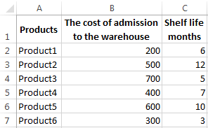
Objective 1. It is necessary to overestimate the trade balances. If he product is kept in stock for more than 8 months we should reduce its price 2 times.
We form a table with initial parameters:
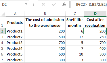
To solve the problem, use the logical IF function. The formula will have a look like this: =IF(C2>=8;B2/2;B2)
Logical expression «C2>=8» is constructed using relational operators «>» and «=». The result of his calculations is a logical value of «TRUE» or «FALSE». In the first case, the function returns the value «B2/2». In the second it’s «B2».
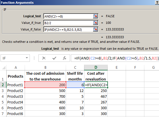
Let’s complicate the task — to employ the logic function И. Now we have such a condition: if the product is stored for more than 8 months, the price is reduced 2 times. If it’s more than 5 months, but less than 8, it’s 1.5 times.
The formula takes the following form:
The use of logic functions in Excel:
| Function Name | Value | Syntax | Note |
| TRUE | It does not have arguments, it returns the logical value » TRUE « | TRUE | It is rarely used as an independent function |
| FALSE | It does not have arguments, it returns the logical value » FALSE « | FALSE | ——-//——- |
| AND | If all the given arguments return true result, then the function issues a logical expression » TRUE «. If one of the function outputs the result «false» the whole function gives the result «FALSE» | =AND(boolean1;boolean2;…) | Accepts up to 255 arguments in the form of conditions or links. It is mandatory to first. |
| OR | It displays the result “TRUE“ if at least one of the arguments is true. | =OR(boolean1;boolean2;…) | ——-//——- |
| NOT | It changes the logic value “TRUE on the contrary — » FALSE «. And vice versa. | #NAME? | Usually it is combined with other operators. |
| IF | Test the validity of a logical expression and returns the result | =IF (boolean;value_if_TRUE;value_if_FALSE) | « boolean » in the calculations should have results “ TRUE “ or “ FALSE “ |
| IFERROR | If the first argument is true, it returns its argument. Otherwise it’s the value of the second argument. | = IFERROR(value;”error”) | Both arguments are mandatory. |
The function IF can be used as arguments to the text values
Objective 2. If the value of the goods in the warehouse after the write-down was less than 300 r. or the product is stored for longer than 10 months, it is written off.
For the solution use logic functions IF and OR:
Condition recorded using a logical OR operation, stands as follows: goods are deducted if the number in cell D2 = 10.
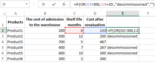
In terms of non-compliance with the conditions, IF function returns to an empty cell.
As arguments, you can use other functions. These are mathematical, for example.
Objective 3. Students before entering the gymnasium pass math, English and Russian. Passing Score is 12. You should get at least 4 points in mathematics for admission. Create report on the receipt.
We set up a table with the source data:
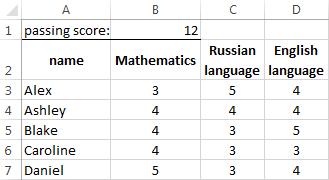
It is necessary to compare the total number of points with a passing grade. And check that math score was not lower than «4». In the «result» column put «accepted» or «not accepted».
There’s such a formula:
Logical operator «AND» causes the function to check the validity of the two conditions. The mathematical function «SUM» is used to calculate the final score.
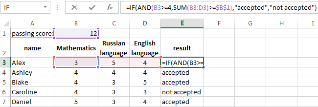
The function IF allows us to solve many problems; it is therefore used more often.
The statistical and logical functions in Excel
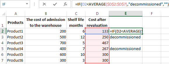
Task 1. Analyze the cost of cash balances after the devaluation. If the price of the product after reassessment is below average values, we should write off the product from the warehouse.
Working with the table in the previous section:
To solve the problem use the formula of such a form:
In logical terms «D2<AVERAGE (D2:D7)» apply statistical function AVERAGE. It returns the average of the range D2: D7.
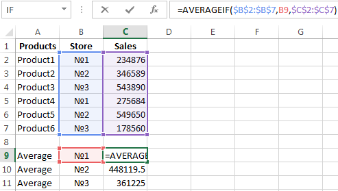
Task 2. Find the average sales in stores.
We set up a table with the source data:
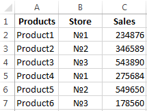
You need to find the arithmetic meaning for the cells, which value corresponds to a predetermined condition. That is to combine logical and statistical solution.
Below a table with a condition there’s the table to display the results.
We solve the problem with a single function:
The first argument $B$2:$B$7 is a range of cells for testing. The second argument B9 is a condition. The third argument the $C$2:$C$7 is an averaging range; the numerical values, which are taken to calculate the arithmetic mean.
AVERAGEIF function compares the value of B9 cells (№1) with values in the range B2: B7. That is the number of stores in the sales table. For matching the data considers the arithmetic mean of using numbers in the range C2: C7.
Task 3. Find the average sales in the store №1 New York and №2 Los Angeles.
Modify the table from the previous example:
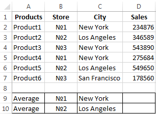
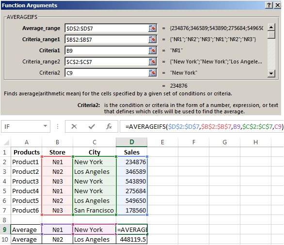
It is necessary to fulfill two conditions — use the function of the form:
Download examples logical functions
The function AVERAGEIFS allows you to use more than one condition. The first argument $D$2:$D$7 is an averaging ranges (where are the numbers to find the arithmetic mean). The second argument $B$2:$B$7 is a range to test the first condition. The third argument B9 is the first condition. The fourth and fifth arguments are the ranges for checking the second condition respectively.
The function takes into account only the values that meet all these criteria.