

Use the Find and Replace features in Excel to search for something in your workbook, such as a particular number or text string. You can either locate the search item for reference, or you can replace it with something else. You can include wildcard characters such as question marks, tildes, and asterisks, or numbers in your search terms. You can search by rows and columns, search within comments or values, and search within worksheets or entire workbooks.

Find
To find something, press Ctrl+F, or go to Home > Editing > Find & Select > Find.
Note: In the following example, we’ve clicked the Options >> button to show the entire Find dialog. By default, it will display with Options hidden.

-
In the Find what: box, type the text or numbers you want to find, or click the arrow in the Find what: box, and then select a recent search item from the list.
Tips: You can use wildcard characters — question mark (?), asterisk (*), tilde (~) — in your search criteria.
-
Use the question mark (?) to find any single character — for example, s?t finds «sat» and «set».
-
Use the asterisk (*) to find any number of characters — for example, s*d finds «sad» and «started».
-
Use the tilde (~) followed by ?, *, or ~ to find question marks, asterisks, or other tilde characters — for example, fy91~? finds «fy91?».
-
-
Click Find All or Find Next to run your search.
Tip: When you click Find All, every occurrence of the criteria that you are searching for will be listed, and clicking a specific occurrence in the list will select its cell. You can sort the results of a Find All search by clicking a column heading.
-
Click Options>> to further define your search if needed:
-
Within: To search for data in a worksheet or in an entire workbook, select Sheet or Workbook.
-
Search: You can choose to search either By Rows (default), or By Columns.
-
Look in: To search for data with specific details, in the box, click Formulas, Values, Notes, or Comments.
Note: Formulas, Values, Notes and Comments are only available on the Find tab; only Formulas are available on the Replace tab.
-
Match case — Check this if you want to search for case-sensitive data.
-
Match entire cell contents — Check this if you want to search for cells that contain just the characters that you typed in the Find what: box.
-
-
If you want to search for text or numbers with specific formatting, click Format, and then make your selections in the Find Format dialog box.
Tip: If you want to find cells that just match a specific format, you can delete any criteria in the Find what box, and then select a specific cell format as an example. Click the arrow next to Format, click Choose Format From Cell, and then click the cell that has the formatting that you want to search for.
Replace
To replace text or numbers, press Ctrl+H, or go to Home > Editing > Find & Select > Replace.
Note: In the following example, we’ve clicked the Options >> button to show the entire Find dialog. By default, it will display with Options hidden.

-
In the Find what: box, type the text or numbers you want to find, or click the arrow in the Find what: box, and then select a recent search item from the list.
Tips: You can use wildcard characters — question mark (?), asterisk (*), tilde (~) — in your search criteria.
-
Use the question mark (?) to find any single character — for example, s?t finds «sat» and «set».
-
Use the asterisk (*) to find any number of characters — for example, s*d finds «sad» and «started».
-
Use the tilde (~) followed by ?, *, or ~ to find question marks, asterisks, or other tilde characters — for example, fy91~? finds «fy91?».
-
-
In the Replace with: box, enter the text or numbers you want to use to replace the search text.
-
Click Replace All or Replace.
Tip: When you click Replace All, every occurrence of the criteria that you are searching for will be replaced, while Replace will update one occurrence at a time.
-
Click Options>> to further define your search if needed:
-
Within: To search for data in a worksheet or in an entire workbook, select Sheet or Workbook.
-
Search: You can choose to search either By Rows (default), or By Columns.
-
Look in: To search for data with specific details, in the box, click Formulas, Values, Notes, or Comments.
Note: Formulas, Values, Notes and Comments are only available on the Find tab; only Formulas are available on the Replace tab.
-
Match case — Check this if you want to search for case-sensitive data.
-
Match entire cell contents — Check this if you want to search for cells that contain just the characters that you typed in the Find what: box.
-
-
If you want to search for text or numbers with specific formatting, click Format, and then make your selections in the Find Format dialog box.
Tip: If you want to find cells that just match a specific format, you can delete any criteria in the Find what box, and then select a specific cell format as an example. Click the arrow next to Format, click Choose Format From Cell, and then click the cell that has the formatting that you want to search for.
There are two distinct methods for finding or replacing text or numbers on the Mac. The first is to use the Find & Replace dialog. The second is to use the Search bar in the ribbon.
Find & Replace dialog
Search bar and options

-
Press Ctrl+F or go to Home > Find & Select > Find.
-
In Find what: type the text or numbers you want to find.
-
Select Find Next to run your search.
-
You can further define your search:
-
Within: To search for data in a worksheet or in an entire workbook, select Sheet or Workbook.
-
Search: You can choose to search either By Rows (default), or By Columns.
-
Look in: To search for data with specific details, in the box, click Formulas, Values, Notes, or Comments.
-
Match case — Check this if you want to search for case-sensitive data.
-
Match entire cell contents — Check this if you want to search for cells that contain just the characters that you typed in the Find what: box.
-
Tips: You can use wildcard characters — question mark (?), asterisk (*), tilde (~) — in your search criteria.
-
Use the question mark (?) to find any single character — for example, s?t finds «sat» and «set».
-
Use the asterisk (*) to find any number of characters — for example, s*d finds «sad» and «started».
-
Use the tilde (~) followed by ?, *, or ~ to find question marks, asterisks, or other tilde characters — for example, fy91~? finds «fy91?».

-
Press Ctrl+F or go to Home > Find & Select > Find.
-
In Find what: type the text or numbers you want to find.
-
Select Find All to run your search for all occurrences.

Note: The dialog box expands to show a list of all the cells that contain the search term, and the total number of cells in which it appears.
-
Select any item in the list to highlight the corresponding cell in your worksheet.
Note: You can edit the contents of the highlighted cell.

-
Press Ctrl+H or go to Home > Find & Select > Replace.
-
In Find what, type the text or numbers you want to find.
-
You can further define your search:
-
Within: To search for data in a worksheet or in an entire workbook, select Sheet or Workbook.
-
Search: You can choose to search either By Rows (default), or By Columns.
-
Match case — Check this if you want to search for case-sensitive data.
-
Match entire cell contents — Check this if you want to search for cells that contain just the characters that you typed in the Find what: box.
Tips: You can use wildcard characters — question mark (?), asterisk (*), tilde (~) — in your search criteria.
-
Use the question mark (?) to find any single character — for example, s?t finds «sat» and «set».
-
Use the asterisk (*) to find any number of characters — for example, s*d finds «sad» and «started».
-
Use the tilde (~) followed by ?, *, or ~ to find question marks, asterisks, or other tilde characters — for example, fy91~? finds «fy91?».
-
-
-
In the Replace with box, enter the text or numbers you want to use to replace the search text.
-
Select Replace or Replace All.
Tips:
-
When you select Replace All, every occurrence of the criteria that you are searching for is replaced.
-
When you select Replace, you can replace one instance at a time by selecting Next to highlight the next instance.
-
-
Select any cell to search the entire sheet or select a specific range of cells to search.
-
Press Command + F or select the magnifying glass to expand the Search bar and type the text or number you want to find in the search field.
Tips: You can use wildcard characters — question mark (?), asterisk (*), tilde (~) — in your search criteria.
-
Use the question mark (?) to find any single character — for example, s?t finds «sat» and «set».
-
Use the asterisk (*) to find any number of characters — for example, s*d finds «sad» and «started».
-
Use the tilde (~) followed by ?, *, or ~ to find question marks, asterisks, or other tilde characters — for example, fy91~? finds «fy91?».
-
-
Press return.
Notes:
-
To find the next instance of the item you are searching for, press return again or use the Find dialog box and select Find Next.
-
To specify additional search options, select the magnifying glass and select Search in Sheet or Search in Workbook. You can also select the Advanced option, which launches the Find dialog.
Tip: You can cancel a search in progress by pressing ESC.
-
Find
To find something, press Ctrl+F, or go to Home > Editing > Find & Select > Find.
Note: In the following example, we’ve clicked > Search Options to show the entire Find dialog. By default, it will display with Search Options hidden.

-
In the Find what: box, type the text or numbers you want to find.
Tips: You can use wildcard characters — question mark (?), asterisk (*), tilde (~) — in your search criteria.
-
Use the question mark (?) to find any single character — for example, s?t finds «sat» and «set».
-
Use the asterisk (*) to find any number of characters — for example, s*d finds «sad» and «started».
-
Use the tilde (~) followed by ?, *, or ~ to find question marks, asterisks, or other tilde characters — for example, fy91~? finds «fy91?».
-
-
Click Find Next or Find All to run your search.
Tip: When you click Find All, every occurrence of the criteria that you are searching for will be listed, and clicking a specific occurrence in the list will select its cell. You can sort the results of a Find All search by clicking a column heading.
-
Click > Search Options to further define your search if needed:
-
Within: To search for data within a certain selection, choose Selection. To search for data in a worksheet or in an entire workbook, select Sheet or Workbook.
-
Direction: You can choose to search either Down (default), or Up.
-
Match case — Check this if you want to search for case-sensitive data.
-
Match entire cell contents — Check this if you want to search for cells that contain just the characters that you typed in the Find what box.
-
Replace
To replace text or numbers, press Ctrl+H, or go to Home > Editing > Find & Select > Replace.
Note: In the following example, we’ve clicked > Search Options to show the entire Find dialog. By default, it will display with Search Options hidden.

-
In the Find what: box, type the text or numbers you want to find.
Tips: You can use wildcard characters — question mark (?), asterisk (*), tilde (~) — in your search criteria.
-
Use the question mark (?) to find any single character — for example, s?t finds «sat» and «set».
-
Use the asterisk (*) to find any number of characters — for example, s*d finds «sad» and «started».
-
Use the tilde (~) followed by ?, *, or ~ to find question marks, asterisks, or other tilde characters — for example, fy91~? finds «fy91?».
-
-
In the Replace with: box, enter the text or numbers you want to use to replace the search text.
-
Click Replace or Replace All.
Tip: When you click Replace All, every occurrence of the criteria that you are searching for will be replaced, while Replace will update one occurrence at a time.
-
Click > Search Options to further define your search if needed:
-
Within: To search for data within a certain selection, choose Selection. To search for data in a worksheet or in an entire workbook, select Sheet or Workbook.
-
Direction: You can choose to search either Down (default), or Up.
-
Match case — Check this if you want to search for case-sensitive data.
-
Match entire cell contents — Check this if you want to search for cells that contain just the characters that you typed in the Find what box.
-
Need more help?
You can always ask an expert in the Excel Tech Community or get support in the Answers community.
Recommended articles
Merge and unmerge cells
REPLACE, REPLACEB functions
Apply data validation to cells
How to Replace Text in Excel with the REPLACE function (2023)
Need to replace text in multiple cells?
Excel’s REPLACE and SUBSTITUTE functions make the process much easier.
Let’s take a look at how the two functions work, how they differ, and how you put them to use in a real spreadsheet🔍
If you want to follow along with what I show you, download my workbook here.
Replacing characters in text with the REPLACE function
The REPLACE function substitutes a text string with another text string.
Let’s say your boss tells you that the product IDs for a product line must be changed.
But only a part of the product ID should be changed – not all of it.

Here, the “29FA” part of all the product IDs needs to be changed to “39LU”.
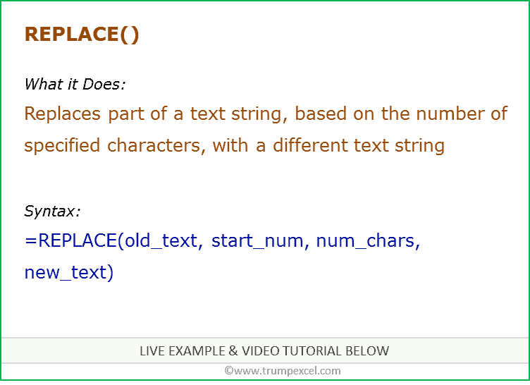
To do that with the REPLACE function, we’ll walk through the syntax of the REPLACE function, which goes like this:
=REPLACE(old_text, start_num, num_chars, new_text)
Don’t worry, it’s not as daunting as it looks. It’s actually pretty straightforward👍
Step 1: Old text
The old text argument is a reference to the cell where you want to replace some text. Write:
=REPLACE(A2

And put a comma to wrap up the first argument, and let’s move on to the next.
Step 2: Start num
The start_num argument determines where the REPLACE function should start replacing characters from.
In our case, the “29FA” part starts on the 3rd character in the text.

So, write:
=REPLACE(A2, 3,
Now, we’ve established where the REPLACE function should start to replace text.
Still with me? Then let’s dive into the next argument of the REPLACE syntax🤿
Step 3: Num chars
Also called the “number of characters” argument, this determines how many characters should be replaced with the new text.
Typically, this should be the length of the text you want to replace the old text with.
So, it ties together with the next argument.
If you want to replace “29FA” with “39LU”, then you’re replacing the next 4 characters.
Write:
=REPLACE(A2, 3, 4

And wrap it up with a comma🎁
There are situations where this num_chars argument should be a different length than the new_text argument. I’ll tell you more about that later.
Step 4: New text
The new_text argument is the replacement text for the old text.
So, simply write the new characters that should replace the old 4 characters:
=REPLACE(A2, 3, 4, “39LU”

Remember the double quotes when the replacement text is letters or a combination of numbers and letters.
Wrap up the formula with an end parenthesis and press Enter.
Now, the “29FA” part of the old product ID is replaced with “39LU”.

PRO TIP: Length of num_chars vs new_text
If you need the replacement text to be shorter or longer than the text it’s replacing, you can have a different length in the 3rd and 4th argument of REPLACE. Let me give you a few formula examples of that:
If you wanted to replace the “29FA” with “39L” instead, you’d write:
=REPLACE(A2, 3, 4, “39L”)
But the length of the 4th argument would be shorter than the 4 characters defined in the 3rd argument.
On the other hand, if you wanted to replace “FA” with “LLUU”, you’d write this:
=REPLACE(A2, 5, 2, “LLUU”)

Replacing text strings with the SUBSTITUTE function
If the string you want to replace doesn’t always appear in the same place, you’re better off using the SUBSTITUTE function.
The syntax of SUBSTITUTE goes like this:
=SUBSTITUTE(text, old_text, new_text, [instance_num])
This is a little different from the last syntax of the REPLACE function, so be careful not to get them mixed up⚠️
Step 1: Text
The text argument is just a cell reference to the cell where you want to replace text.
Write:
=SUBSTITUTE(A2

And of course, put a comma to go to the next argument.
Step 2: Old text
The SUBSTITUTE function doesn’t replace characters from a fixed position in a cell.
Instead, it cleverly searches for a text string and begins replacing characters from there🔍
So, if you want to replace the “FA” part of the product ID with “LU”, write:
=SUBSTITUTE(A2, “FU”

Step 3: New text
The new_text argument is what the old text should be replaced with.
For this example, that’s “LU”.
=SUBSTITUTE(A2, “FA”, “LU”

The new text doesn’t have to be the same length as the old text.
Step 4: Instance num
The optional instance num argument decides how many times the text should be replaced.
This is relevant if there is more than one instance of the old text.
The instance_num argument is optional. If you leave it blank, every instance of the old text is replaced by the new text😊
In the following formula example, the first 2 product IDs each have 2 instances of the “FA”. So, the instance num argument determines whether only the first instance of “FA” is replaced with “LU” or both instances of “FA” is replaced with “LU”.
As you can see from the picture below, write 1 if you want only the first instance of “FA” to be replaced.
=SUBSTITUTE(A2, “FA”, “LU”, 1)
Or don’t use the instance num argument if every instance of “FA” should be replaced:
=SUBSTITUTE(A2, “FA”, “LU”)

And that’s how to replace text dynamically based on the location of the text you want to replace.
The difference between REPLACE and SUBSTITUTE
There are a few subtle differences between these two “replace functions”.
Both of them replace one or more characters in a text string with another text string.
The difference lies in how the first string is identified.
REPLACE selects the first string based on the position. So you might replace four characters, starting with the sixth character in the string.
SUBSTITUTE selects based on whether the string matches a predefined search. You might tell Excel to replace any instance of “FA” with “LU” for example.
Other than that, the two functions are identical👬🏻
Replace text using Find and Replace
Another way to replace text is with the ‘Find and Replace’ feature of Excel.
It’s a way to substitute characters in the original cell instead of having to add additional columns with formulas.
1. Select all the cells that contain the text to replace.
2. From the ‘Home’ tab, click ‘ Find and Select’.

3. From the Find and Replace dialog box (in the replace tab) write the text you want to replace, in the ‘Find what:’ field.
4. Still within the ‘Find and Replace’ dialog box, write the new text to replace the old text with in the ‘Replace with:’ field.

5. When you click the ‘Replace all’ button, Excel replaces all instances of the old text with the new text, in the selected cells.
If you instead want to replace all instances of the text within the entire workbook, just select a single cell before opening the ‘Find and Replace’ dialog box.
(Instead of selecting multiple cells).
That’s it – Now what?
With the REPLACE and SUBSTITUTE functions, you can replace very specific strings with other strings. You can use letters, numbers, or other characters.
In short, you can replace text with extreme accuracy. And that saves you a great deal of time when you need to make a lot of edits.
Additionally, you can use the Find and Replace tool, which is the most underrated feature of Excel.
But no one got a job offer just based on their skills to replace characters in a text in Microsoft Excel.
Luckily, there are other areas of Excel that are magnets for job offers🧲
Click here to learn IF, SUMIF, VLOOKUP, and pivot tables (yup, that’s the magnets) for FREE in my 30-minute online Excel course.
Other resources
Replacing text is often used to clean up data so it’s ready for analysis, formulas, pivot tables, etc.
Other ways of cleaning up data are with other important Excel functions like LEFT, RIGHT, MID, and LEN.
Or with one of the two ways of deleting blank rows (one better than the other). Read all about it here.
Kasper Langmann2023-01-19T12:24:59+00:00
Page load link
In this tutorial, I will show you how to use the REPLACE function in Excel (with examples).
Replace is a text function that allows you to quickly replace a string or a part of the string with some other text string.
This can be really useful when you’re working with a large dataset and you want to replace or remove a part of the string. But the real power of the replace function can be unleashed when you use it with other formulas in Excel (as we will in the examples covered later in this tutorial).
Before I show you the examples of using the function, let me quickly cover the syntax of the REPLACE function.
Syntax of the REPLACE Function
=REPLACE(old_text, start_num, num_chars, new_text)
Input Arguments
- old_text – the text that you want to replace.
- start_num – the starting position from where the search should begin.
- num_chars – the number of characters to replace.
- new_text – the new text that should replace the old_text.
Note that the Start Number and Number of Characters argument cannot be negative.
Now let’s have a look at some examples to see how the REPLACE function can be used in Excel.
Example 1 – Replace Text with Blank
Suppose you have the following data set and you want to replace the text “ID-” and only want to keep the numeric part.

You can do this by using the following formula:
=REPLACE(A2,1,3,"")
The above formula replaces the first three characters of the text in each cell with a blank.

Note: The same result can also be achieved by other techniques such as using the Find and Replace or by extracting the text to the right of the dash by using the combination of RIGHT and FIND functions.
Example 2: Extract the User Name from the Domain name
Suppose you have a dataset as shown below and you want to remove the domain part (the one that follows the @ sign).

To do this, you can use the below formula:
=REPLACE(A2,FIND("@",A2),LEN(A2)-FIND("@",A2)+1,"")

The above function uses a combination of REPLACE, LEN and FIND function.
It first uses the FIND function to get the position of the @. This value is used as the Start Number argument and I want to remove the entire text string starting from the @ sign.
Another thing I need to remove this string is the total number of characters after the @ so that I can specify these many characters to be replaced with a blank. This is where I have used the formula combination of LEN and FIND.
Pro Tip: In the above formula, since I want to remove all the characters after the @ sign, I don’t really need the number of characters. I can specify any large number (which is greater than the number of characters after the @ sign), and I will get the same result. So I can even use the following formula: =REPLACE(A2,FIND(“@”,A2),LEN(A2),””)
Example 3: Replace One Text String with Another
In the above two examples, I showed you how to extract a part of the string by replacing the remaining with blank.
Here is an example where you change one text string with another.
Suppose you have the below dataset and you want to change the domain from example.net to example.com.

You can do this using the below formula:
=REPLACE(A2,FIND("net",A2),3,"com")

Difference between Replace and Substitute functions
There is a major difference in the usage of the REPLACE function and the SUBSTITUTE function (although the result expected from these may be similar).
The REPLACE function requires the position from which it needs to start replacing the text. It then also requires the number of characters you need to replace with the new text. This makes REPLACE function suitable where you have a clear pattern in the data and want to replace text.
A good example of this could be when working with email ids or address or ids – where the construct of the text is consistent.
SUBSTITUTE function, on the other hand, is a little more versatile. You can use it to replace all the instances of an occurrence of a string with some other string.
For example, I can use it to replace all the occurrence of character Z with J in a text string. And at the same time, it also gives you the flexibility to only change a specific instance of the occurrence (for example, only substitute the first occurrence of the matching string or only the second occurrence).
Note: In many cases, you can do away with using the REPLACE function and instead use the FIND and REPLACE functionality. It will allow you to change the data set without using the formula and getting the result in another column/row. REPLACE function is more suited when you want to keep the original dataset and also want the resulting data to be dynamic (such that updates in case you change the original data).
Excel REPLACE Function – Video Tutorial
Related Excel Functions:
- Excel FIND Function.
- Excel LOWER Function.
- Excel UPPER Function.
- Excel PROPER Function.
- Excel SEARCH Function.
You may also like the following Excel Tutorials:
- How to Remove the First Character from a String in Excel
Purpose
Replace text based on content
Usage notes
The Excel SUBSTITUTE function can replace text by matching. Use the SUBSTITUTE function when you want to replace text based on matching, not position. Optionally, you can specify the instance of found text to replace (i.e. first instance, second instance, etc.).
SUBSTITUTE is case-sensitive. To replace one or more characters with nothing, enter an empty string («»).
Examples
Below are the formulas used in the example shown above:
=SUBSTITUTE(B5,"t","b") // replace all t's with b's
=SUBSTITUTE(B6,"t","b",1) // replace first t with b
=SUBSTITUTE(B7,"cat","dog") // replace cat with dog
=SUBSTITUTE(B8,"&","") // replace # with nothing
=SUBSTITUTE(B9,"-",", ") // replace hyphen with comma
The SUBSTITUTE function cannot replace more than one string at a time. However, SUBSTITUTE can be nested inside of itself to accomplish the same thing. For example, with the text «a (dog)» in cell A1, the formula below will strip parentheses () from text:
=SUBSTITUTE(SUBSTITUTE(A1,"(",""),")","") // returns "a dog"
This same approach can be used in a more complex formula to normalize telephone numbers.
Related functions
Use the REPLACE function to replace text at a known location in a text string. Use the SUBSTITUTE function to replace text by searching when the location is not known. Use FIND or SEARCH to determine the location of specific text.
Notes
- SUBSTITUTE finds and replaces old_text with new_text in a text string.
- Instance limits SUBSTITUTE replacement a particular instance of old_text.
- When instance is omitted, all instances of old_text are replaced with new_text.
- SUBSTITUTE is case-sensitive and does not support wildcards.
Замена части строкового выражения в VBA Excel по указанному шаблону поиска и замены и возврат преобразованной строки с помощью функции Replace.
Replace – это функция, которая возвращает строку, полученную в результате замены одной подстроки в исходном строковом выражении другой подстрокой указанное количество раз.
Если замену подстроки необходимо осуществить в диапазоне ячеек, функцию Replace следует применить к значению каждой ячейки заданного диапазона. Проще замену в диапазоне ячеек произвести с помощью метода Range.Replace.
Синтаксис и параметры
Replace(expression, find, replace, [start], [count], [compare])
- expression – исходное строковое выражение, содержащее подстроку, которую необходимо заменить;
- find – искомая подстрока, подлежащая замене;
- replace – подстрока, заменяющая искомую подстроку;
- start – порядковый номер символа исходной строки, с которого необходимо начать поиск, часть строки до этого номера обрезается, по умолчанию равен 1 (необязательный параметр);
- count – количество замен подстроки, по умолчанию выполняется замена всех обнаруженных вхождений (необязательный параметр);
- compare – числовое значение, указывающее вид сравнения (необязательный параметр).
Сокращенный синтаксис функции Replace с необязательными параметрами по умолчанию:
Replace(expression, find, replace)
Параметр compare
| Константа | Значение | Описание |
|---|---|---|
| vbUseCompareOption | -1 | используется параметр, заданный оператором Option Compare |
| vbBinaryCompare | 0 | выполняется двоичное сравнение |
| vbTextCompare | 1 | применяется текстовое сравнение |
По умолчанию используется двоичное (бинарное) сравнение. При таком сравнении буквенные символы в нижнем и верхнем регистрах различаются. Если необходимо провести замену подстроки независимо от регистра букв, используйте значение параметра compare – vbTextCompare (1).
Примеры кода VBA Excel
Пример 1
Замена единственного вхождения искомой подстроки в строковое выражение:
|
Sub Primer1() Dim a a = «Сливочное масло» a = Replace(a, «Сливочное», «Рыжиковое») MsgBox a ‘Результат: «Рыжиковое масло» End Sub |
Пример 2
Замена нескольких вхождений искомой подстроки в строковое выражение:
|
Sub Primer2() Dim a a = «Идёт медведь, идёт лиса, идёт грач» ‘с параметром compare по умолчанию a = Replace(a, «идёт», «бежит») MsgBox a ‘Результат: ‘Идёт медведь, бежит лиса, бежит грач a = «Идёт медведь, идёт лиса, идёт грач» ‘с параметром compare=1(vbTextCompare) a = Replace(a, «идёт», «бежит», , , 1) MsgBox a ‘Результат: ‘бежит медведь, бежит лиса, бежит грач End Sub |
Пример 3
Замена одного вхождения искомой подстроки в строковое выражение из нескольких с обрезанием исходной строки до 15 символа:
|
Sub Primer3() Dim a a = «Идёт медведь, идёт лиса, идёт грач» a = Replace(a, «идёт», «бежит», 15, 1) MsgBox a ‘Результат: ‘бежит лиса, идёт грач End Sub |