

Use the Find and Replace features in Excel to search for something in your workbook, such as a particular number or text string. You can either locate the search item for reference, or you can replace it with something else. You can include wildcard characters such as question marks, tildes, and asterisks, or numbers in your search terms. You can search by rows and columns, search within comments or values, and search within worksheets or entire workbooks.

Find
To find something, press Ctrl+F, or go to Home > Editing > Find & Select > Find.
Note: In the following example, we’ve clicked the Options >> button to show the entire Find dialog. By default, it will display with Options hidden.

-
In the Find what: box, type the text or numbers you want to find, or click the arrow in the Find what: box, and then select a recent search item from the list.
Tips: You can use wildcard characters — question mark (?), asterisk (*), tilde (~) — in your search criteria.
-
Use the question mark (?) to find any single character — for example, s?t finds «sat» and «set».
-
Use the asterisk (*) to find any number of characters — for example, s*d finds «sad» and «started».
-
Use the tilde (~) followed by ?, *, or ~ to find question marks, asterisks, or other tilde characters — for example, fy91~? finds «fy91?».
-
-
Click Find All or Find Next to run your search.
Tip: When you click Find All, every occurrence of the criteria that you are searching for will be listed, and clicking a specific occurrence in the list will select its cell. You can sort the results of a Find All search by clicking a column heading.
-
Click Options>> to further define your search if needed:
-
Within: To search for data in a worksheet or in an entire workbook, select Sheet or Workbook.
-
Search: You can choose to search either By Rows (default), or By Columns.
-
Look in: To search for data with specific details, in the box, click Formulas, Values, Notes, or Comments.
Note: Formulas, Values, Notes and Comments are only available on the Find tab; only Formulas are available on the Replace tab.
-
Match case — Check this if you want to search for case-sensitive data.
-
Match entire cell contents — Check this if you want to search for cells that contain just the characters that you typed in the Find what: box.
-
-
If you want to search for text or numbers with specific formatting, click Format, and then make your selections in the Find Format dialog box.
Tip: If you want to find cells that just match a specific format, you can delete any criteria in the Find what box, and then select a specific cell format as an example. Click the arrow next to Format, click Choose Format From Cell, and then click the cell that has the formatting that you want to search for.
Replace
To replace text or numbers, press Ctrl+H, or go to Home > Editing > Find & Select > Replace.
Note: In the following example, we’ve clicked the Options >> button to show the entire Find dialog. By default, it will display with Options hidden.

-
In the Find what: box, type the text or numbers you want to find, or click the arrow in the Find what: box, and then select a recent search item from the list.
Tips: You can use wildcard characters — question mark (?), asterisk (*), tilde (~) — in your search criteria.
-
Use the question mark (?) to find any single character — for example, s?t finds «sat» and «set».
-
Use the asterisk (*) to find any number of characters — for example, s*d finds «sad» and «started».
-
Use the tilde (~) followed by ?, *, or ~ to find question marks, asterisks, or other tilde characters — for example, fy91~? finds «fy91?».
-
-
In the Replace with: box, enter the text or numbers you want to use to replace the search text.
-
Click Replace All or Replace.
Tip: When you click Replace All, every occurrence of the criteria that you are searching for will be replaced, while Replace will update one occurrence at a time.
-
Click Options>> to further define your search if needed:
-
Within: To search for data in a worksheet or in an entire workbook, select Sheet or Workbook.
-
Search: You can choose to search either By Rows (default), or By Columns.
-
Look in: To search for data with specific details, in the box, click Formulas, Values, Notes, or Comments.
Note: Formulas, Values, Notes and Comments are only available on the Find tab; only Formulas are available on the Replace tab.
-
Match case — Check this if you want to search for case-sensitive data.
-
Match entire cell contents — Check this if you want to search for cells that contain just the characters that you typed in the Find what: box.
-
-
If you want to search for text or numbers with specific formatting, click Format, and then make your selections in the Find Format dialog box.
Tip: If you want to find cells that just match a specific format, you can delete any criteria in the Find what box, and then select a specific cell format as an example. Click the arrow next to Format, click Choose Format From Cell, and then click the cell that has the formatting that you want to search for.
There are two distinct methods for finding or replacing text or numbers on the Mac. The first is to use the Find & Replace dialog. The second is to use the Search bar in the ribbon.
Find & Replace dialog
Search bar and options

-
Press Ctrl+F or go to Home > Find & Select > Find.
-
In Find what: type the text or numbers you want to find.
-
Select Find Next to run your search.
-
You can further define your search:
-
Within: To search for data in a worksheet or in an entire workbook, select Sheet or Workbook.
-
Search: You can choose to search either By Rows (default), or By Columns.
-
Look in: To search for data with specific details, in the box, click Formulas, Values, Notes, or Comments.
-
Match case — Check this if you want to search for case-sensitive data.
-
Match entire cell contents — Check this if you want to search for cells that contain just the characters that you typed in the Find what: box.
-
Tips: You can use wildcard characters — question mark (?), asterisk (*), tilde (~) — in your search criteria.
-
Use the question mark (?) to find any single character — for example, s?t finds «sat» and «set».
-
Use the asterisk (*) to find any number of characters — for example, s*d finds «sad» and «started».
-
Use the tilde (~) followed by ?, *, or ~ to find question marks, asterisks, or other tilde characters — for example, fy91~? finds «fy91?».

-
Press Ctrl+F or go to Home > Find & Select > Find.
-
In Find what: type the text or numbers you want to find.
-
Select Find All to run your search for all occurrences.

Note: The dialog box expands to show a list of all the cells that contain the search term, and the total number of cells in which it appears.
-
Select any item in the list to highlight the corresponding cell in your worksheet.
Note: You can edit the contents of the highlighted cell.

-
Press Ctrl+H or go to Home > Find & Select > Replace.
-
In Find what, type the text or numbers you want to find.
-
You can further define your search:
-
Within: To search for data in a worksheet or in an entire workbook, select Sheet or Workbook.
-
Search: You can choose to search either By Rows (default), or By Columns.
-
Match case — Check this if you want to search for case-sensitive data.
-
Match entire cell contents — Check this if you want to search for cells that contain just the characters that you typed in the Find what: box.
Tips: You can use wildcard characters — question mark (?), asterisk (*), tilde (~) — in your search criteria.
-
Use the question mark (?) to find any single character — for example, s?t finds «sat» and «set».
-
Use the asterisk (*) to find any number of characters — for example, s*d finds «sad» and «started».
-
Use the tilde (~) followed by ?, *, or ~ to find question marks, asterisks, or other tilde characters — for example, fy91~? finds «fy91?».
-
-
-
In the Replace with box, enter the text or numbers you want to use to replace the search text.
-
Select Replace or Replace All.
Tips:
-
When you select Replace All, every occurrence of the criteria that you are searching for is replaced.
-
When you select Replace, you can replace one instance at a time by selecting Next to highlight the next instance.
-
-
Select any cell to search the entire sheet or select a specific range of cells to search.
-
Press Command + F or select the magnifying glass to expand the Search bar and type the text or number you want to find in the search field.
Tips: You can use wildcard characters — question mark (?), asterisk (*), tilde (~) — in your search criteria.
-
Use the question mark (?) to find any single character — for example, s?t finds «sat» and «set».
-
Use the asterisk (*) to find any number of characters — for example, s*d finds «sad» and «started».
-
Use the tilde (~) followed by ?, *, or ~ to find question marks, asterisks, or other tilde characters — for example, fy91~? finds «fy91?».
-
-
Press return.
Notes:
-
To find the next instance of the item you are searching for, press return again or use the Find dialog box and select Find Next.
-
To specify additional search options, select the magnifying glass and select Search in Sheet or Search in Workbook. You can also select the Advanced option, which launches the Find dialog.
Tip: You can cancel a search in progress by pressing ESC.
-
Find
To find something, press Ctrl+F, or go to Home > Editing > Find & Select > Find.
Note: In the following example, we’ve clicked > Search Options to show the entire Find dialog. By default, it will display with Search Options hidden.

-
In the Find what: box, type the text or numbers you want to find.
Tips: You can use wildcard characters — question mark (?), asterisk (*), tilde (~) — in your search criteria.
-
Use the question mark (?) to find any single character — for example, s?t finds «sat» and «set».
-
Use the asterisk (*) to find any number of characters — for example, s*d finds «sad» and «started».
-
Use the tilde (~) followed by ?, *, or ~ to find question marks, asterisks, or other tilde characters — for example, fy91~? finds «fy91?».
-
-
Click Find Next or Find All to run your search.
Tip: When you click Find All, every occurrence of the criteria that you are searching for will be listed, and clicking a specific occurrence in the list will select its cell. You can sort the results of a Find All search by clicking a column heading.
-
Click > Search Options to further define your search if needed:
-
Within: To search for data within a certain selection, choose Selection. To search for data in a worksheet or in an entire workbook, select Sheet or Workbook.
-
Direction: You can choose to search either Down (default), or Up.
-
Match case — Check this if you want to search for case-sensitive data.
-
Match entire cell contents — Check this if you want to search for cells that contain just the characters that you typed in the Find what box.
-
Replace
To replace text or numbers, press Ctrl+H, or go to Home > Editing > Find & Select > Replace.
Note: In the following example, we’ve clicked > Search Options to show the entire Find dialog. By default, it will display with Search Options hidden.

-
In the Find what: box, type the text or numbers you want to find.
Tips: You can use wildcard characters — question mark (?), asterisk (*), tilde (~) — in your search criteria.
-
Use the question mark (?) to find any single character — for example, s?t finds «sat» and «set».
-
Use the asterisk (*) to find any number of characters — for example, s*d finds «sad» and «started».
-
Use the tilde (~) followed by ?, *, or ~ to find question marks, asterisks, or other tilde characters — for example, fy91~? finds «fy91?».
-
-
In the Replace with: box, enter the text or numbers you want to use to replace the search text.
-
Click Replace or Replace All.
Tip: When you click Replace All, every occurrence of the criteria that you are searching for will be replaced, while Replace will update one occurrence at a time.
-
Click > Search Options to further define your search if needed:
-
Within: To search for data within a certain selection, choose Selection. To search for data in a worksheet or in an entire workbook, select Sheet or Workbook.
-
Direction: You can choose to search either Down (default), or Up.
-
Match case — Check this if you want to search for case-sensitive data.
-
Match entire cell contents — Check this if you want to search for cells that contain just the characters that you typed in the Find what box.
-
Need more help?
You can always ask an expert in the Excel Tech Community or get support in the Answers community.
Recommended articles
Merge and unmerge cells
REPLACE, REPLACEB functions
Apply data validation to cells
![]()
Download Article
![]()
Download Article
This wikiHow will show you how to find and replace cell values in Microsoft Excel. The Find and Replace tool is available in all versions of Excel, including the mobile Excel app.
-
1
Open your workbook in Excel. You can open your project by clicking the File menu and selecting Open. You can also open it by right-clicking the file and selecting Open With > Excel.
- This method should work for all versions of Microsoft Excel beginning with Excel 2007.
-
2
Click the Home tab. You’ll find this in the editing menu above your document.
Advertisement
-
3
Click Find & Select. You’ll find this in the «Editing» grouping of the Home tab with the icon of a magnifying glass.
-
4
Click Replace. This is usually the first listing in the drop-down menu.
-
5
Enter the original value in the «Find what» text box field. This is the text that will be replaced.
- You can use * to find a string of characters. For example, s*d will find «sad» as well as «started.»[1]
- You can use ? to replace a single character in a search. For example, s?t will find «sat» and «set.»[2]
- You can use * to find a string of characters. For example, s*d will find «sad» as well as «started.»[1]
-
6
Enter the new value in the «Replace with» text box field. This text will replace the original text.
- You can opt to match the case, so you can change every instance of «wikihow» to «wikiHow.»
- You can chose to contain your find and replace to the current worksheet or apply it to the entire workbook.
-
7
Click Replace All or Replace. If you want to decide to replace each original value individually, choose Replace, but if you want to replace all the original values at once, choose replace all.[3]


Advertisement
-
1
Open your project in Excel. This app icon looks like a green-and-white spreadsheet icon with an «X» next to it. You can find this app on the Home screen, in the app drawer, or by searching.
- If you don’t have the Excel app, you can get it for free from the App Store (iOS) and the Google Play Store (Android).
- Tap the Open tab in Excel to find all your recent documents.
-
2
Tap the search icon
that looks like a magnifying glass. You’ll see this in the top right corner of your screen.
- A search bar will appear at the top of your document.
-
3
Tap the gear icon
. You’ll see this next to the search bar that dropped down. Search options will appear.
-
4
Tap to select Find and Replace or Find and Replace All. As you tap an option, you’ll see the search bar at the top of the screen change to fit your selection.
- Tap Find and Replace if you want to replace each original value individually.
- Tap Find and Replace All if you want to replace all the original values instantly.
-
5
Tap Done (iOS) or X (Android). You’ll see this option at the top right of the search settings.
-
6
Type your original value into the «Find» bar. This is the current value located in your document.
-
7
Type the new value into the «Replace» bar. This value will replace the current value in the document.
-
8
Tap Replace or Replace All. You’ll see this with your «find and replace» terms.


Advertisement
Ask a Question
200 characters left
Include your email address to get a message when this question is answered.
Submit
Advertisement
Thanks for submitting a tip for review!
wikiHow Video: How to Replace Values in Excel
References
About This Article
Article SummaryX
To find and replace cell values on your computer, open your worksheet in Excel and click the Home tab. Click the Find & Select button on the toolbar, and then select Replace on the menu. On the «»Find and Replace»» window, enter the text you want to find into the «»Find what»» field. You can even use wildcards for a string of text. Wildcards are special characters that replace other characters in searches, like a question mark in place of a letter or an asterisk. In the «»Replace with»» field, type your replacement text exactly how it should appear. To replace all original values at once, click the Replace All button. If you’d rather approve each replacement, click Replace instead.
To replace cell values in the mobile Excel app, open Excel and select a file to edit. Tap the search icon at the top-right corner, and then tap the gear icon next to the search bar to view your options. If you want to replace multiple instances of the same text all at once, tap Find and Replace All. If you’d rather manually approve each replacement, select Replace instead. Then, Tap Done at the top-right corner. Now, type the text you want to replace into the «»Find»» bar, and the replacement text into the «»Replace»» bar. Finally, tap Replace or ‘Replace All to replace the cell values.
Did this summary help you?
Thanks to all authors for creating a page that has been read 18,609 times.
Is this article up to date?
Quickly Fill Blanks with Zeros or Other Values in Excel Worksheets (0, -, N/A, Null or Other Text)
by Avantix Learning Team | Updated August 7, 2021
Applies to: Microsoft® Excel® 2010, 2013, 2016, 2019 and 365 (Windows)
You can quickly replace blank cells in Excel with zeros, dashes or other number or text values (0, -, N/A, Null or other text). It’s useful to fill blank cells with a number, symbol or value if you want to use the data set as the source for a pivot table or use other data analysis tools.
Recommended article: How to Delete Blank Rows in Excel (5 Easy Ways with Shortcuts)
Do you want to learn more about Excel? Check out our virtual classroom or live classroom Excel courses >
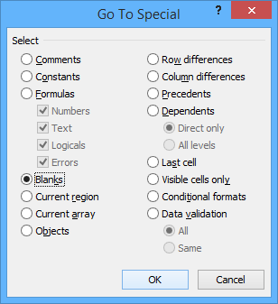
Below is the Go To Special dialog box in Excel:
To quickly replace blanks in an Excel range and fill with zeros, dashes or other values:
- Select the range of cells with blank cells you want to replace.
- Press Ctrl + G to display the Go To dialog box and then click Special to display the Go To Special dialog box. Alternatively, you can click the Home tab in the Ribbon and then select Go to Special from the Find & Select drop-down menu.
- Select Blanks in the Go To Special dialog box and click OK. Excel will select all of the blank cells within the range.
- Type the value you want to enter in the blanks (such as 0, – or text). The value will be entered in the active cell. You can also type the value in the Formula Bar.
- Press Ctrl + Enter. The zero, dash or other value will be inserted in all of the selected blank cells.
This article was first published on December 11, 2020 and has been updated for clarity and content.
Subscribe to get more articles like this one
Did you find this article helpful? If you would like to receive new articles, join our email list.
More resources
How to Use Flash Fill in Excel (4 Ways with Shortcuts)
3 Excel Strikethrough Shortcuts to Cross Out Text or Values in Cells
How to Replace Blank Cells in Excel with a Value from the Cell Above
How to Quickly Delete Blank Rows in Excel (5 Fast Ways to Remove Empty Rows)
10 Excel Flash Fill Examples (Extract, Combine, Clean and Format Data with Flash Fill)
Related courses
Microsoft Excel: Intermediate / Advanced
Microsoft Excel: Data Analysis with Functions, Dashboards and What-If Analysis Tools
Microsoft Excel: Introduction to Visual Basic for Applications (VBA)
VIEW MORE COURSES >
Our instructor-led courses are delivered in virtual classroom format or at our downtown Toronto location at 18 King Street East, Suite 1400, Toronto, Ontario, Canada (some in-person classroom courses may also be delivered at an alternate downtown Toronto location). Contact us at info@avantixlearning.ca if you’d like to arrange custom instructor-led virtual classroom or onsite training on a date that’s convenient for you.
Copyright 2023 Avantix® Learning
Microsoft, the Microsoft logo, Microsoft Office and related Microsoft applications and logos are registered trademarks of Microsoft Corporation in Canada, US and other countries. All other trademarks are the property of the registered owners.
Avantix Learning |18 King Street East, Suite 1400, Toronto, Ontario, Canada M5C 1C4 | Contact us at info@avantixlearning.ca
Excel REPLACE Function (Table of Contents)
- REPLACE in Excel
- How to Use REPLACE Function in Excel?
REPLACE in Excel
Replace function in excel by which we can replace any portion of a cell content by selecting the start and last word till we want to replace it with the word in the same syntax. This is as easy as using Find and Replace operational function.
REPLACE Formula in Excel
Below is the REPLACE Formula in Excel:
The REPLACE function in Excel has the below arguments:
- Old_text (Compulsory or required parameter): The cell reference contains the text you want to replace. (It may contain text or numeric data)
- Start_Num (Compulsory or required parameter): It is the starting position from where the search should begin, i.e. From the left side of the character in the old_text argument
- Num_chars (Compulsory or required parameter): It is the number of characters you want to replace.
- new_text (Compulsory or required parameter): It is the new text that you’d like to replace the old_text
Note: the new_text argument does not need to be similar or the same length as num_chars.
How to use REPLACE Function in Excel?
REPLACE Function is very simple to use. Let us now see how to use REPLACE function in Excel with the help of some examples.
You can download this REPLACE Function Excel Template here – REPLACE Function Excel Template
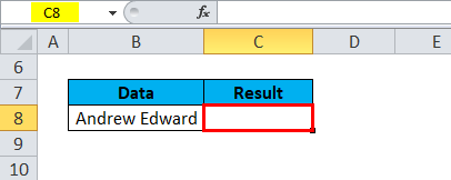
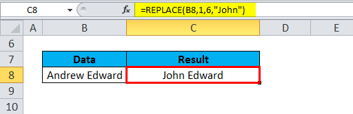
Example #1 – REPLACE Function for Name Change
The below-mentioned example, Cell “B8”, it contains the name “Andrew Edward”. Here I need to REPLACE that name with the correct name, i.e. John Edward, with the help of REPLACE function.
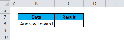
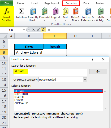
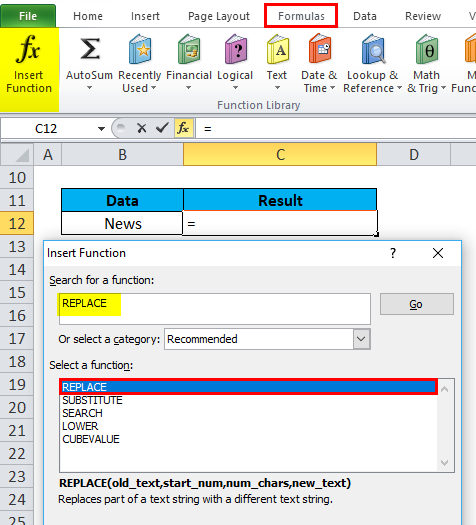
Let’s apply to REPLACE function in cell “C8”. Select the cell “C8” where REPLACE function needs to be applied.
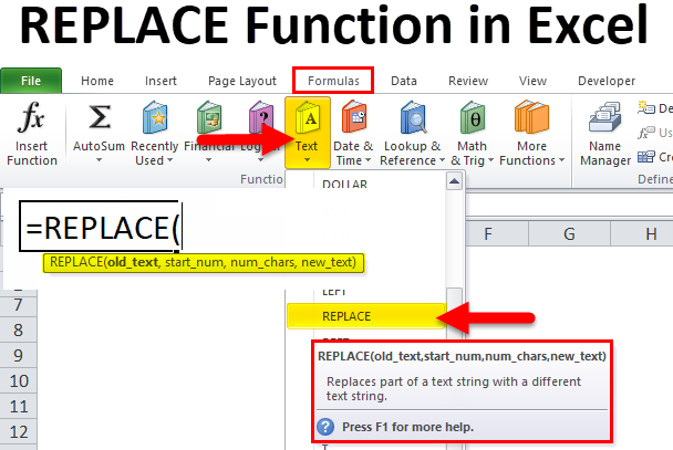
Click the insert function button (fx) under the formula toolbar, a dialog box will appear, type the keyword “REPLACE” in the search for a function box, REPLACE function will appear in the select a function box. Double click on REPLACE function.
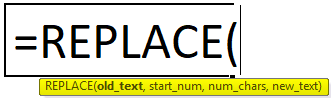
A dialog box appears where arguments for REPLACE function needs to be filled or entered i.e.
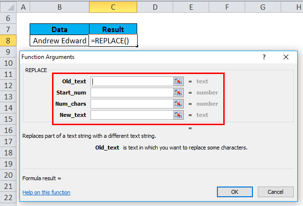
=REPLACE(old_text, start_num, num_chars, new_text)
- Old_text: is the cell reference containing the text which you want to replace. i.e. “B8” or “Andrew Edward.”
- Start_Num: It is the starting position from where the search should begin, i.e. From the left side of the character in the old_text argument, i.e. 1
- Num_chars or Number_of_chars: It is the number of characters you want to replace. i.e. The word ANDREW contains 6 letters which I need to replace; therefore, it is 6
- new_text: The new text you’d like to replace the old_text, here “John” is a new string & “Andrew” is the old string. i.e. Here, we have to enter a new string, i.e. “John.”
Click ok after entering all the replace function arguments.
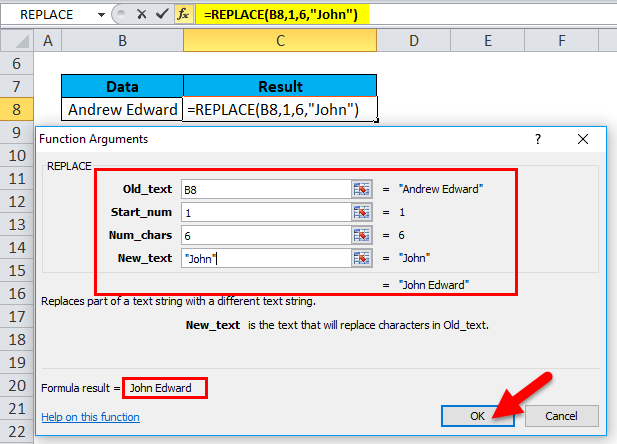
=REPLACE(B8,1,6,”John”)
It replaces text in a specified position of a given or supplied string, i.e. John Edward in cell C8
Example #2 – Addition Of Missing Word In A Text
In the below-mentioned example, In the cell “B12”, it contains the word “News”. Here I need to add the missing word, i.e. “Paper”. With the help of REPLACE function.
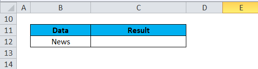
Let’s apply to REPLACE function in cell “C12”. Select the cell “C12” where REPLACE function needs to be applied,
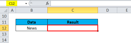
Click the insert function button (fx) under the formula toolbar, a dialog box will appear, type the keyword “REPLACE” in the search for a function box, REPLACE function will appear in the select a function box. Double click on REPLACE function.
A dialog box appears where arguments for REPLACE function needs to be filled or entered i.e.
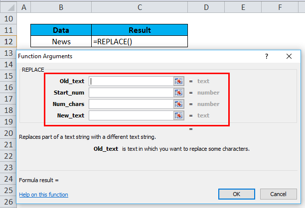
=REPLACE(old_text, start_num, num_chars, new_text)
- Old_text: is the cell reference containing the text which you want to replace. i.e. “B12” or “News.”
- Start_Num: From the left side of the character in old_text argument (News), i.e. 5, from 5th position, add a New_text
- Num_chars or Number_of_chars: Here, it is left blank. i.e. We are not replacing anything here, as we are adding a missing word to old_text.
- New_text: We are not replacing anything here; here, “ Paper” is a new string. Therefore, we have to enter a new string that has to be added to that old text. i.e. “ Paper”
Note: We had to add one space before the word “paper.”
Click ok after entering all the replace function arguments.
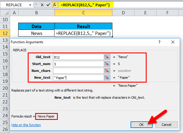
=REPLACE(B12,5,,” Paper”)
It adds the new text in a specified position, i.e. “News Paper” in cell C12.

Example #3 – Addition Of Hyphen In Phone Number
In the below-mentioned example, Cell “G8” contains a contact number with state code “0224038991”. Here I need to add a hyphen after state code with the help of replace function. i.e. “022-4038991.”
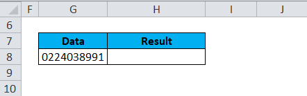
Let’s apply to REPLACE function in cell “H8”. Select the cell “H8” where REPLACE function needs to be applied.
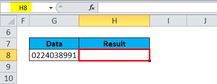
Click the insert function button (fx) under the formula toolbar, a dialog box will appear, type the keyword “REPLACE” in the search for a function box, REPLACE function will appear in the select a function box. Double click on REPLACE function.
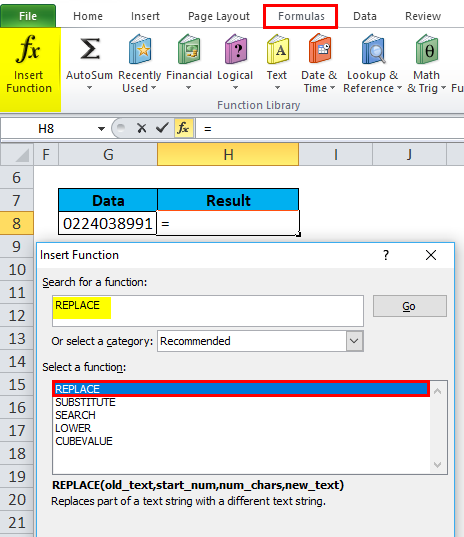
A dialog box appears where arguments for REPLACE function needs to be filled or entered i.e.
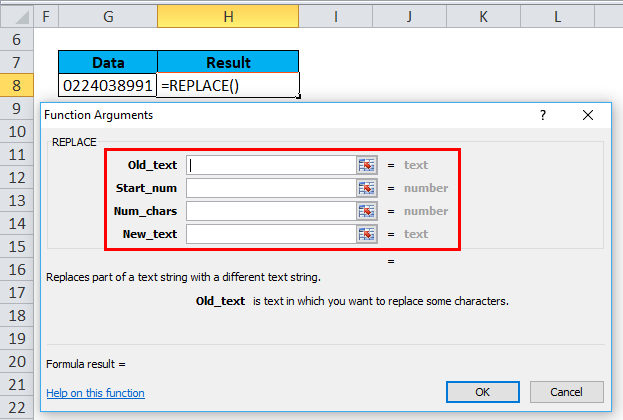
=REPLACE(old_text, start_num, num_chars, new_text)
- Old_text: is the cell reference containing the text which you want to replace. i.e. “G8” or “0224038991.”
- Start_Num: From the left side of the character in the old_text argument, i.e. 4. At 4th position, add hyphen “-”
- Num_chars or Number_of_chars: Here, it is left blank. i.e. We are not replacing anything here, as we are adding Hyphen in between contact number
- New_text: We are not replacing anything here, “ – ” i.e. Hyphen is a special character or new string Which has to be added in between an old string
Note: We had to add one space before & after the hyphen “ – ” to get the desired result
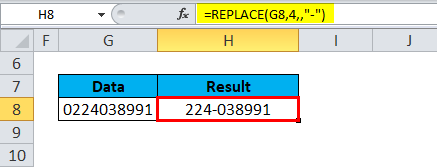
Click ok, after entering all the arguments in replace function.
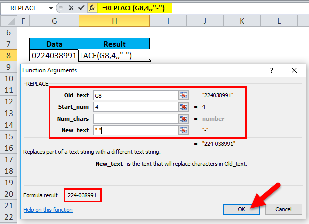
=REPLACE(“0224038991″,4,,” – “)
It replaces the hyphen “-” in a specified position, i.e. “022-4038991” in cell C12.
Things to Remember
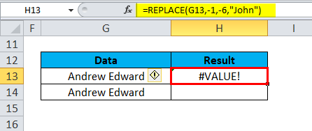
#VALUE error occurs if start_num or num_chars argument is a non-numeric or negative value.
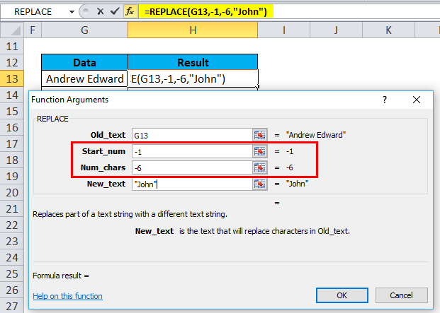
It will throw a Value Error.
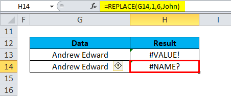
#NAME error Occurs if the Old_text argument is not enclosed in double quotation marks
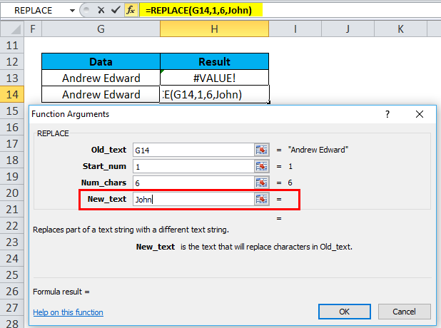
It will throw a Name Error.
Recommended Articles
This has been a guide to REPLACE in Excel. Here we discuss the REPLACE Formula and how to use REPLACE function in Excel along with practical examples and a downloadable excel template. You can also go through our other suggested articles –
- Excel DAY Function
- YEAR Function in Excel
- Find and Replace in Excel
- REPLACE Formula in Excel
REPLACE function is included in the text functions of MS Excel and is intended to replace a specific area of the text string containing the source text on the specified text line (new text).
How does the REPLACE function in Excel work?
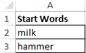
Example 1. In order to study in detail the operation of this function, we consider one of the simplest examples. Suppose we have several words in different columns, we need to get new words using the original ones. For this example, in addition to our main function REPLACE, we also use the RIGHT function — this function serves to return a certain number of characters from the end of a line of text. That is, for example, we have two words: milk and a skating rink, as a result we must get the word hammer.
REPLACE function in Excel and examples of its use
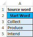
- Create a table with words on the sheet of the Excel spreadsheet workbook, as shown in the figure:
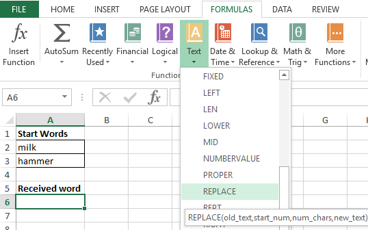
- Next, on the sheet of the workbook, we will prepare an area for placing our result — the resulting word “hammer”, as shown below. Place the cursor in cell A6 and call the function REPLACE:
- Fill the function with the arguments shown in the figure:
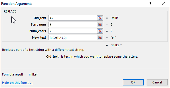
Let us explain the choice of these parameters as follows: cell A2 was chosen as the beginning of the text, the number 5 was set as beginning_, since it is from the fifth position of the word “Milk” we don’t take characters for our final word, the number_ of signs was set equal to 2, since this number It is not taken into account in the new word, as the new text, the set option RIGHT with the parameters of the cell A3 and taking the last two characters «ok».
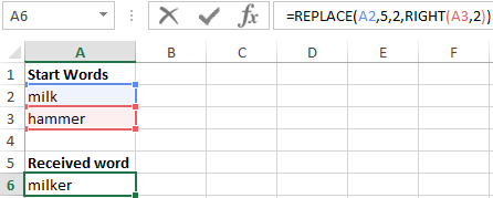
Next, click on the «OK» button and get the result:
How to REPLACE a piece of text in Excel cell?
Example 2. Consider another small example. Suppose we have columns of words in the cells of the Excel spreadsheet. It is necessary to replace their letters in certain places so as to convert them.
- Let’s create a tablet with words on the sheet of an Excel workbook, as shown in the figure:
- Further, on the same sheet of the working book we will prepare an area for placing our result — modified words. Fill the cells with two types of formulas as shown in the picture:
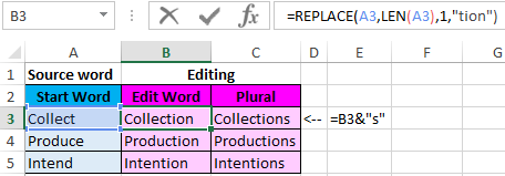
Download examples text function REPLACE in Excel
Note! In the second formula, we use the operator “&” to add the character «s» to the male surname to convert it to the female. To solve this problem, one could use the function =CONCATENATE(B3,»s») instead of the formula =B3&»s» — the result is identical. But today it is strongly recommended to abandon this formula as it has its limitations and is more demanding on resources in comparison with a simple and convenient ampersand operator.