
Excel for Microsoft 365 Excel for Microsoft 365 for Mac Excel for the web Excel 2021 Excel 2021 for Mac Excel 2019 Excel 2019 for Mac Excel 2016 Excel 2016 for Mac Excel 2013 Excel 2010 Excel 2007 Excel for Mac 2011 Excel Starter 2010 More…Less
This article describes the formula syntax and usage of the REPLACE and REPLACEB
function in Microsoft Excel.
Description
REPLACE replaces part of a text string, based on the number of characters you specify, with a different text string.
REPLACEB replaces part of a text string, based on the number of bytes you specify, with a different text string.
Important:
-
These functions may not be available in all languages.
-
REPLACE is intended for use with languages that use the single-byte character set (SBCS), whereas REPLACEB is intended for use with languages that use the double-byte character set (DBCS). The default language setting on your computer affects the return value in the following way:
-
REPLACE always counts each character, whether single-byte or double-byte, as 1, no matter what the default language setting is.
-
REPLACEB counts each double-byte character as 2 when you have enabled the editing of a language that supports DBCS and then set it as the default language. Otherwise, REPLACEB counts each character as 1.
The languages that support DBCS include Japanese, Chinese (Simplified), Chinese (Traditional), and Korean.
Syntax
REPLACE(old_text, start_num, num_chars, new_text)
REPLACEB(old_text, start_num, num_bytes, new_text)
The REPLACE and REPLACEB function syntax has the following arguments:
-
Old_text Required. Text in which you want to replace some characters.
-
Start_num Required. The position of the character in old_text that you want to replace with new_text.
-
Num_chars Required. The number of characters in old_text that you want REPLACE to replace with new_text.
-
Num_bytes Required. The number of bytes in old_text that you want REPLACEB to replace with new_text.
-
New_text Required. The text that will replace characters in old_text.
Example
Copy the example data in the following table, and paste it in cell A1 of a new Excel worksheet. For formulas to show results, select them, press F2, and then press Enter. If you need to, you can adjust the column widths to see all the data.
|
Data |
||
|
abcdefghijk |
||
|
2009 |
||
|
123456 |
||
|
Formula |
Description (Result) |
Result |
|
=REPLACE(A2,6,5,»*») |
Replaces five characters in abcdefghijk with a single * character, starting with the sixth character (f). |
abcde*k |
|
=REPLACE(A3,3,2,»10″) |
Replaces the last two digits (09) of 2009 with 10. |
2010 |
|
=REPLACE(A4,1,3,»@») |
Replaces the first three characters of 123456 with a single @ character. |
@456 |
Need more help?
Want more options?
Explore subscription benefits, browse training courses, learn how to secure your device, and more.
Communities help you ask and answer questions, give feedback, and hear from experts with rich knowledge.
Purpose
Replace text based on content
Usage notes
The Excel SUBSTITUTE function can replace text by matching. Use the SUBSTITUTE function when you want to replace text based on matching, not position. Optionally, you can specify the instance of found text to replace (i.e. first instance, second instance, etc.).
SUBSTITUTE is case-sensitive. To replace one or more characters with nothing, enter an empty string («»).
Examples
Below are the formulas used in the example shown above:
=SUBSTITUTE(B5,"t","b") // replace all t's with b's
=SUBSTITUTE(B6,"t","b",1) // replace first t with b
=SUBSTITUTE(B7,"cat","dog") // replace cat with dog
=SUBSTITUTE(B8,"&","") // replace # with nothing
=SUBSTITUTE(B9,"-",", ") // replace hyphen with comma
The SUBSTITUTE function cannot replace more than one string at a time. However, SUBSTITUTE can be nested inside of itself to accomplish the same thing. For example, with the text «a (dog)» in cell A1, the formula below will strip parentheses () from text:
=SUBSTITUTE(SUBSTITUTE(A1,"(",""),")","") // returns "a dog"
This same approach can be used in a more complex formula to normalize telephone numbers.
Related functions
Use the REPLACE function to replace text at a known location in a text string. Use the SUBSTITUTE function to replace text by searching when the location is not known. Use FIND or SEARCH to determine the location of specific text.
Notes
- SUBSTITUTE finds and replaces old_text with new_text in a text string.
- Instance limits SUBSTITUTE replacement a particular instance of old_text.
- When instance is omitted, all instances of old_text are replaced with new_text.
- SUBSTITUTE is case-sensitive and does not support wildcards.
The SUBSTITUTE function in Microsoft Excel is a handy tool that enables users to replace single or multiple instances of a specific character or text string with a different character or text string. To see how this works on a spreadsheet, we will discuss the syntax and four arguments of the Excel SUBSTITUTE function.
Next, we will try our hand at some SUBSTITUTE formulas by working through a couple of examples. SUBSTITUTE is an in-built worksheet function categorized as a String/Text function in Excel. The SUBSTITUTE function is case-sensitive and does not support wildcard characters.

Syntax
=SUBSTITUTE(text, old_text, new_text, [nth_instance])
Arguments:
text – This is a required argument where you will input the original text string within which you wish to substitute the character(s) supplied through the old_text argument. To supply a value for this argument, you may use a cell reference, enter a text string, or use a return supplied by another formula.
old_text – This is a required argument where you will input the character(s) or text string you wish to substitute.
new_text – This is a required argument where you will input the character(s) or text string you wish to substitute the contents of old_text argument with.
nth_instance – This is an optional argument that lets you instruct Excel as to which instance of the character(s) or text string in the old_text argument you will like to replace. If omitted, the function will substitute all instances of the character(s) or text string entered in the old_text argument.
Important Characteristics of the SUBSTITUTE function
- SUBSTITUTE function is a helpful tool that enables you to replace specific character(s) or text string by entering them in the
old_textargument, with character(s) or text string entered in thenew_text - The optional
nth_instanceargument enables you to choose a specific instance of the character(s) or text string entered in theold_textThe omission of this argument will result in the replacement of allold_textinstances with character(s) or text string supplied in thenew_textargument. - SUBSTITUTE is a case-sensitive function and does not support wildcard characters.
Examples of the Excel SUBSTITUTE function
Here are some basic examples of how you can incorporate and use the SUBSTITUTE function in your worksheet. To get a firm hold on the workings of these formulas, pull up a spreadsheet and try using these formulas alongside, as you read through the examples.
1. Substitute all Instances of a String or a Character

=SUBSTITUTE(A2,"1","3")
Let’s break down the formula’s instructions to Excel and see what it looks like using words. In effect, we are asking Excel to: Look at the contents in cell A2 (text argument) and locate all the «1»s (old_text argument) in that cell. Next, substitute all instances of «1» (since we did not supply the nth_instance argument) with «3» (new_text argument).
Here, Excel will substitute all instances of «1» and return «Floor 3, Room 3».
2. Substitute a Specific Instance of a String or a Character

=SUBSTITUTE(A2,"1","3", 2)
This is the same formula we used in the previous example, but with the nth_instance argument supplied as 2. The nth_instance argument will restrict the substitution to only the specified instance, which in our example is the 2nd instance of «1». Therefore, the function will only substitute the 2nd instance and return «Floor 1, Room 3».
3. Case-sensitivity of the SUBSTITUTE function

=SUBSTITUTE(A2,"Room","Chamber")
Vs.
=SUBSTITUTE(A2,"room","Chamber")
Notice how the formula substitutes text string only when you enter the appropriate case. Using «room» instead of «Room» results in no substitution at all.
4. Nested SUBSTITUTE formula

=SUBSTITUTE(SUBSTITUTE(A2,"Floor","Floor No."), "Room", "Room No.")
A nested SUBSTITUTE formula allows us to replace multiple text strings using a single formula. For example, let’s assume we want to add a text string «No.» after both «Floor» and «Room». We would need to use the following formulas:
=SUBSTITUTE(A2,"Floor","Floor No.")
And
=SUBSTITUTE(A2,"Room","Room No.")
Instead, we merge these formulas and nest one SUBSTITUTE formula into another like shown above. The nested formula will involve 2 steps.
- Step-1: It will first work on the «nested» formula, i.e. the one inside the brackets of the first SUBSTITUTE formula. So, the formula will first compute the return for substitution of the text string «Floor» with «Floor No.» At this point, this is what the return looks like: «Floor No.1, Room 1»
- Step-2: Next, the second SUBSTITUTE formula, i.e. the one outside the brackets, looks for the text string «Room» in «Floor No.1, Room 1» (which is the return from step 1) and substitutes «Room» with «Room No.» to give us our desired return:»Floor No.1, Room No.1″
Excel REPLACE Function
Excel REPLACE function is very similar to the SUBSTITUTE function, it can be used for replacing a sequence of characters in a string/text with another set of characters. Let’s briefly go over the syntax of this function.
Syntax
=REPLACE(old_text, start, number_of_chars, new_text)
Arguments:
old_text – The original string value works the same way as in the SUBSTITUTE function.start – The second argument is the position of the character(s) you want to replace.number_of_chars – The third argument is where you input the number of character(s) you want to replace, starting from the position mentioned in the second argument.new_text – The fourth argument is similar to the SUBSTITUTE function’s new_text argument. It is the text string you want to replace the specified character(s) with.
Example of Excel Replace Function:
The only difference between the SUBSTITUTE and REPLACE function is the method of identifying the strings that need to be substituted or replaced. Let’s work through an example of the REPLACE function to see how it uses a different method to accomplish a purpose similar to that of the SUBSTITUTE function.

=REPLACE(A2,"7","1","2")
As we can see, the formula returns «Floor 2, Room 1» since we replaced the «1» with «2». Notice how the REPLACE function does not allow specifying which instance of a particular character or text string we want to replace. It makes intuitive sense because we are already entering the position of the character rather than matching a specified character(s) or text string like with the SUBSTITUTE function.
SUBSTITUTE VS REPLACE – When to choose Which?
If you do not know the specific character(s) of the text string you want to replace, but know the position of those character(s) in the text string, use the REPLACE function. If regardless of the position, you want to change the character(s) in the text string by matching a specified text string, use the SUBSTITUTE function.
I hope these examples gave you a good insight into how you can use the SUBSTITUTE function in your worksheets. Spend a little time with these formulas, and you will champion them in no time. I will see you soon with another powerful Excel function.
Excel REPLACE Function (Table of Contents)
- REPLACE in Excel
- How to Use REPLACE Function in Excel?
REPLACE in Excel
Replace function in excel by which we can replace any portion of a cell content by selecting the start and last word till we want to replace it with the word in the same syntax. This is as easy as using Find and Replace operational function.
REPLACE Formula in Excel
Below is the REPLACE Formula in Excel:
The REPLACE function in Excel has the below arguments:
- Old_text (Compulsory or required parameter): The cell reference contains the text you want to replace. (It may contain text or numeric data)
- Start_Num (Compulsory or required parameter): It is the starting position from where the search should begin, i.e. From the left side of the character in the old_text argument
- Num_chars (Compulsory or required parameter): It is the number of characters you want to replace.
- new_text (Compulsory or required parameter): It is the new text that you’d like to replace the old_text
Note: the new_text argument does not need to be similar or the same length as num_chars.
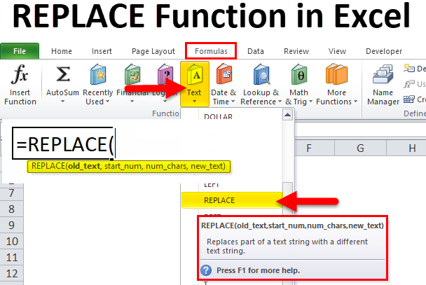
How to use REPLACE Function in Excel?
REPLACE Function is very simple to use. Let us now see how to use REPLACE function in Excel with the help of some examples.
You can download this REPLACE Function Excel Template here – REPLACE Function Excel Template
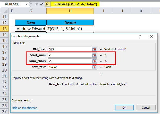
Example #1 – REPLACE Function for Name Change
The below-mentioned example, Cell “B8”, it contains the name “Andrew Edward”. Here I need to REPLACE that name with the correct name, i.e. John Edward, with the help of REPLACE function.
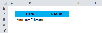
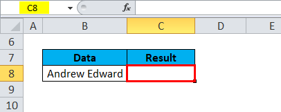
Let’s apply to REPLACE function in cell “C8”. Select the cell “C8” where REPLACE function needs to be applied.
Click the insert function button (fx) under the formula toolbar, a dialog box will appear, type the keyword “REPLACE” in the search for a function box, REPLACE function will appear in the select a function box. Double click on REPLACE function.
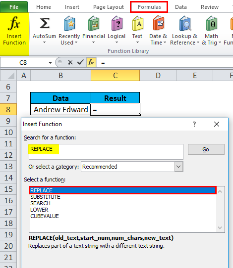
A dialog box appears where arguments for REPLACE function needs to be filled or entered i.e.
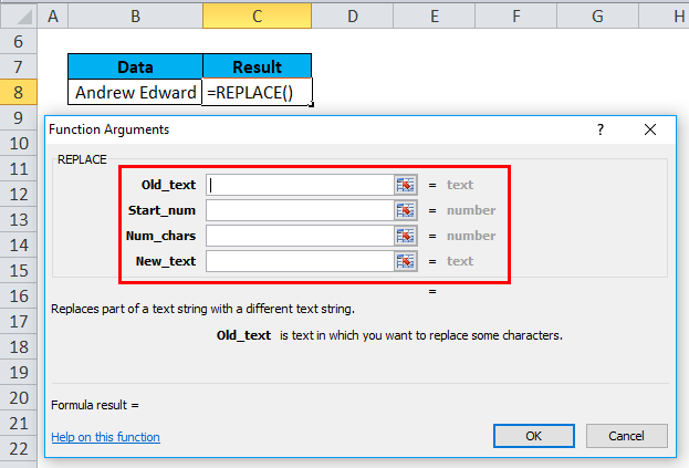
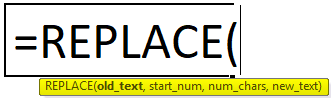
=REPLACE(old_text, start_num, num_chars, new_text)
- Old_text: is the cell reference containing the text which you want to replace. i.e. “B8” or “Andrew Edward.”
- Start_Num: It is the starting position from where the search should begin, i.e. From the left side of the character in the old_text argument, i.e. 1
- Num_chars or Number_of_chars: It is the number of characters you want to replace. i.e. The word ANDREW contains 6 letters which I need to replace; therefore, it is 6
- new_text: The new text you’d like to replace the old_text, here “John” is a new string & “Andrew” is the old string. i.e. Here, we have to enter a new string, i.e. “John.”
Click ok after entering all the replace function arguments.
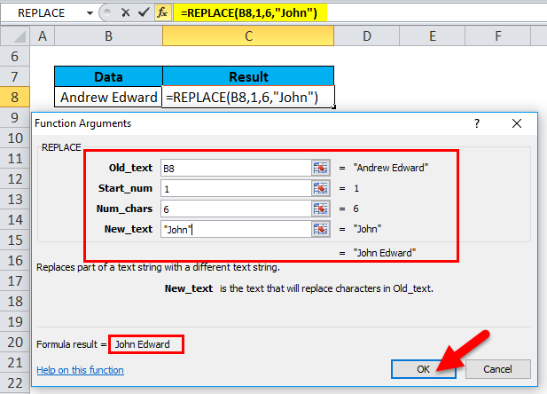
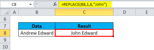
=REPLACE(B8,1,6,”John”)
It replaces text in a specified position of a given or supplied string, i.e. John Edward in cell C8
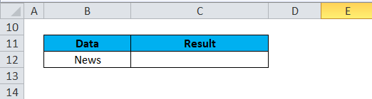
Example #2 – Addition Of Missing Word In A Text
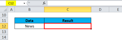
In the below-mentioned example, In the cell “B12”, it contains the word “News”. Here I need to add the missing word, i.e. “Paper”. With the help of REPLACE function.
Let’s apply to REPLACE function in cell “C12”. Select the cell “C12” where REPLACE function needs to be applied,
Click the insert function button (fx) under the formula toolbar, a dialog box will appear, type the keyword “REPLACE” in the search for a function box, REPLACE function will appear in the select a function box. Double click on REPLACE function.
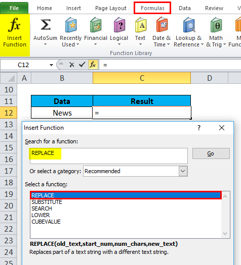
A dialog box appears where arguments for REPLACE function needs to be filled or entered i.e.
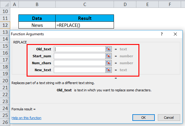
=REPLACE(old_text, start_num, num_chars, new_text)
- Old_text: is the cell reference containing the text which you want to replace. i.e. “B12” or “News.”
- Start_Num: From the left side of the character in old_text argument (News), i.e. 5, from 5th position, add a New_text
- Num_chars or Number_of_chars: Here, it is left blank. i.e. We are not replacing anything here, as we are adding a missing word to old_text.
- New_text: We are not replacing anything here; here, “ Paper” is a new string. Therefore, we have to enter a new string that has to be added to that old text. i.e. “ Paper”
Note: We had to add one space before the word “paper.”
Click ok after entering all the replace function arguments.
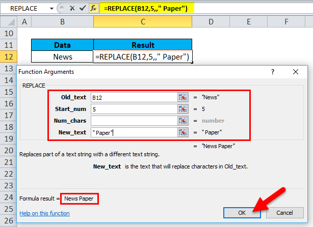
=REPLACE(B12,5,,” Paper”)
It adds the new text in a specified position, i.e. “News Paper” in cell C12.

Example #3 – Addition Of Hyphen In Phone Number
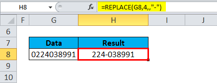
In the below-mentioned example, Cell “G8” contains a contact number with state code “0224038991”. Here I need to add a hyphen after state code with the help of replace function. i.e. “022-4038991.”
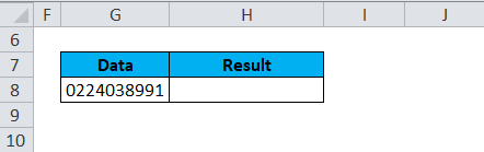
Let’s apply to REPLACE function in cell “H8”. Select the cell “H8” where REPLACE function needs to be applied.
Click the insert function button (fx) under the formula toolbar, a dialog box will appear, type the keyword “REPLACE” in the search for a function box, REPLACE function will appear in the select a function box. Double click on REPLACE function.
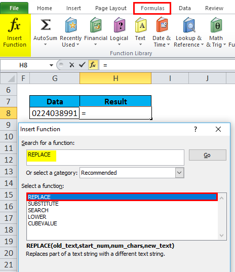
A dialog box appears where arguments for REPLACE function needs to be filled or entered i.e.
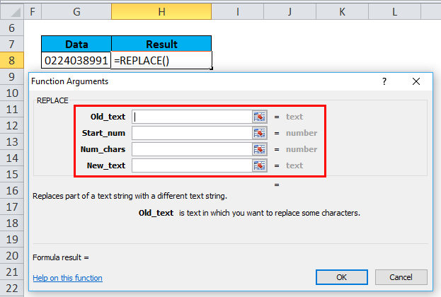
=REPLACE(old_text, start_num, num_chars, new_text)
- Old_text: is the cell reference containing the text which you want to replace. i.e. “G8” or “0224038991.”
- Start_Num: From the left side of the character in the old_text argument, i.e. 4. At 4th position, add hyphen “-”
- Num_chars or Number_of_chars: Here, it is left blank. i.e. We are not replacing anything here, as we are adding Hyphen in between contact number
- New_text: We are not replacing anything here, “ – ” i.e. Hyphen is a special character or new string Which has to be added in between an old string
Note: We had to add one space before & after the hyphen “ – ” to get the desired result
Click ok, after entering all the arguments in replace function.
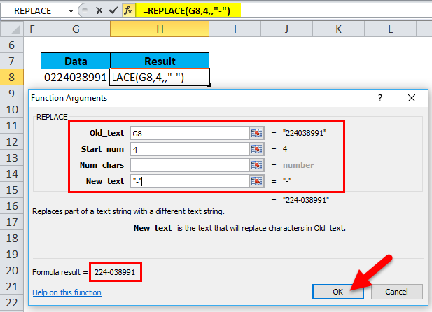
=REPLACE(“0224038991″,4,,” – “)
It replaces the hyphen “-” in a specified position, i.e. “022-4038991” in cell C12.
Things to Remember
#VALUE error occurs if start_num or num_chars argument is a non-numeric or negative value.
It will throw a Value Error.
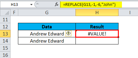
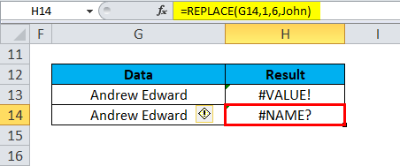
#NAME error Occurs if the Old_text argument is not enclosed in double quotation marks
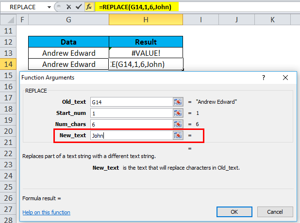
It will throw a Name Error.
Recommended Articles
This has been a guide to REPLACE in Excel. Here we discuss the REPLACE Formula and how to use REPLACE function in Excel along with practical examples and a downloadable excel template. You can also go through our other suggested articles –
- Excel DAY Function
- YEAR Function in Excel
- Find and Replace in Excel
- REPLACE Formula in Excel