
Excel for Microsoft 365 Excel for Microsoft 365 for Mac Excel for the web Excel 2021 Excel 2021 for Mac Excel 2019 Excel 2019 for Mac Excel 2016 Excel 2016 for Mac Excel 2013 Excel 2010 Excel 2007 Excel for Mac 2011 Excel Starter 2010 More…Less
This article describes the formula syntax and usage of the REPLACE and REPLACEB
function in Microsoft Excel.
Description
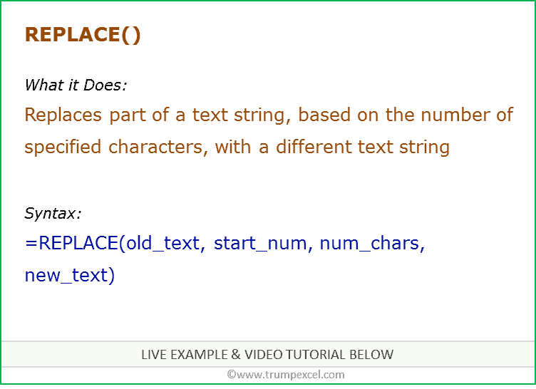
REPLACE replaces part of a text string, based on the number of characters you specify, with a different text string.
REPLACEB replaces part of a text string, based on the number of bytes you specify, with a different text string.
Important:
-
These functions may not be available in all languages.
-
REPLACE is intended for use with languages that use the single-byte character set (SBCS), whereas REPLACEB is intended for use with languages that use the double-byte character set (DBCS). The default language setting on your computer affects the return value in the following way:
-
REPLACE always counts each character, whether single-byte or double-byte, as 1, no matter what the default language setting is.
-
REPLACEB counts each double-byte character as 2 when you have enabled the editing of a language that supports DBCS and then set it as the default language. Otherwise, REPLACEB counts each character as 1.
The languages that support DBCS include Japanese, Chinese (Simplified), Chinese (Traditional), and Korean.
Syntax
REPLACE(old_text, start_num, num_chars, new_text)
REPLACEB(old_text, start_num, num_bytes, new_text)
The REPLACE and REPLACEB function syntax has the following arguments:
-
Old_text Required. Text in which you want to replace some characters.
-
Start_num Required. The position of the character in old_text that you want to replace with new_text.
-
Num_chars Required. The number of characters in old_text that you want REPLACE to replace with new_text.
-
Num_bytes Required. The number of bytes in old_text that you want REPLACEB to replace with new_text.
-
New_text Required. The text that will replace characters in old_text.
Example
Copy the example data in the following table, and paste it in cell A1 of a new Excel worksheet. For formulas to show results, select them, press F2, and then press Enter. If you need to, you can adjust the column widths to see all the data.
|
Data |
||
|
abcdefghijk |
||
|
2009 |
||
|
123456 |
||
|
Formula |
Description (Result) |
Result |
|
=REPLACE(A2,6,5,»*») |
Replaces five characters in abcdefghijk with a single * character, starting with the sixth character (f). |
abcde*k |
|
=REPLACE(A3,3,2,»10″) |
Replaces the last two digits (09) of 2009 with 10. |
2010 |
|
=REPLACE(A4,1,3,»@») |
Replaces the first three characters of 123456 with a single @ character. |
@456 |
Need more help?
Want more options?
Explore subscription benefits, browse training courses, learn how to secure your device, and more.
Communities help you ask and answer questions, give feedback, and hear from experts with rich knowledge.
REPLACE function is included in the text functions of MS Excel and is intended to replace a specific area of the text string containing the source text on the specified text line (new text).
How does the REPLACE function in Excel work?
Example 1. In order to study in detail the operation of this function, we consider one of the simplest examples. Suppose we have several words in different columns, we need to get new words using the original ones. For this example, in addition to our main function REPLACE, we also use the RIGHT function — this function serves to return a certain number of characters from the end of a line of text. That is, for example, we have two words: milk and a skating rink, as a result we must get the word hammer.
REPLACE function in Excel and examples of its use
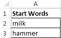
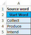
- Create a table with words on the sheet of the Excel spreadsheet workbook, as shown in the figure:
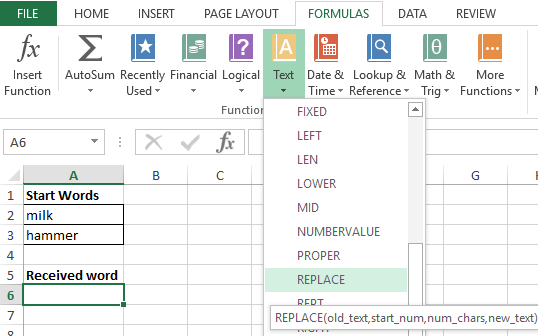
- Next, on the sheet of the workbook, we will prepare an area for placing our result — the resulting word “hammer”, as shown below. Place the cursor in cell A6 and call the function REPLACE:
- Fill the function with the arguments shown in the figure:
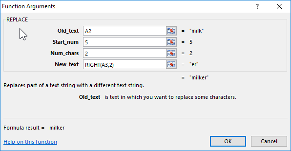
Let us explain the choice of these parameters as follows: cell A2 was chosen as the beginning of the text, the number 5 was set as beginning_, since it is from the fifth position of the word “Milk” we don’t take characters for our final word, the number_ of signs was set equal to 2, since this number It is not taken into account in the new word, as the new text, the set option RIGHT with the parameters of the cell A3 and taking the last two characters «ok».
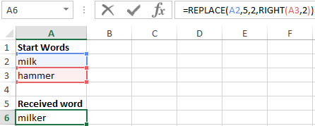
Next, click on the «OK» button and get the result:
How to REPLACE a piece of text in Excel cell?
Example 2. Consider another small example. Suppose we have columns of words in the cells of the Excel spreadsheet. It is necessary to replace their letters in certain places so as to convert them.
- Let’s create a tablet with words on the sheet of an Excel workbook, as shown in the figure:
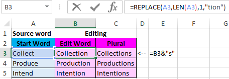
- Further, on the same sheet of the working book we will prepare an area for placing our result — modified words. Fill the cells with two types of formulas as shown in the picture:
Download examples text function REPLACE in Excel
Note! In the second formula, we use the operator “&” to add the character «s» to the male surname to convert it to the female. To solve this problem, one could use the function =CONCATENATE(B3,»s») instead of the formula =B3&»s» — the result is identical. But today it is strongly recommended to abandon this formula as it has its limitations and is more demanding on resources in comparison with a simple and convenient ampersand operator.
The REPLACE function replaces the specified number of characters from the string based on the starting position with the mentioned text, string, or value. The REPLACE function is a text function; therefore, the return value is always in text format.
The REPLACE function can also be used to remove a part of the string by simply swapping the text with an empty string.

Syntax
The REPLACE function accepts four arguments, and all of them are mandatory. The syntax is as follows.
=REPLACE(old_text, start_num, num_chars, new_text)
Arguments:
Understand each argument to be able to use the REPLACE function efficiently.
‘old_text‘ – This is the input text which we wish to replace. The value of old_text can be inserted directly in double quotes or using a cell reference.
‘start_num‘ – This argument suggests the character’s starting position in the input text from where we want to replace the text.
‘num_chars‘ – The number of characters we want to replace from the input text.
‘new_text‘ – This argument contains the value of the replacement text or characters. The new text value that we wish to swap the old one with.
Important Characteristics of the REPLACE Function
One of the most basic aspects of the REPLACE function is that it counts each character, number, alphabet, and space as 1, irrespective of the language setting of the laptop. Other noteworthy features of the REPLACE function are mentioned below.
- Even if the value of the old_text argument is in numerical format, the REPLACE function swaps the character as required, but the return value will be in text format.
- When the value of the start_num argument is less than or equal to zero, the REPLACE function gives a #VALUE error.
- A non-numeric value used as start_num or num_chars returns a #NAME? error.
- The REPLACE function returns a #VALUE error if the value of the num_chars argument is negative.
- If the text value of new_text is not enclosed in double quotes, the function returns a #NAME? error.
Examples of REPLACE Function
As the REPLACE function accepts several arguments, let’s understand the basic functionality with the help of an example.
Example 1 – Basic Functionality of REPLACE Function
In this example, we have taken sample data of a full name, address, and phone number to understand how the REPLACE function behaves with different input text.

In the first example, we are simply replacing one character at the 1st position with the letter «S». As we can see in the return value in cell B3, one character at the first position, which is the letter ‘T’ is replaced with the letter ‘S’. Similarly, in the second example, we intend to replace 4 characters starting from the 1st position with «XXXX», as seen in the return value in cell B4.
In the third example, the input value is in a numerical format, and we are trying to replace 1 character in the 4th position, which is «5», with «@». The return value is as expected but is now in text format, which is evident due to its left alignment.
Hopefully, the basic functionality of the REPLACE function is clear now. In the examples below, we will learn more about its applications.
Example 2 – Replacing Text when Location is Known
There are instances when companies rebrand by altering how they write their brand names or changing the name entirely. Recently, Facebook rebranded itself by changing its name to Meta. In this example, we have a few facts about Facebook, but after the rebranding, the term ‘Facebook’ must be replaced with ‘Meta’.
Doing it manually is a daunting task and inefficient. Instead, we can use the REPLACE function to our advantage.

The formula used will be as follows.
=REPLACE(B3,1,8,"Meta")

As the word that needs to be replaced is at the beginning of the string, it is easier to use the REPLACE function as the value of the start_num argument can be 1 for all the strings. We also know the length of the text that needs to be replaced, which is ‘Facebook’; therefore, the value of the num_chars is 8.
In the above scenario, the position of the word to be replaced was known, and it was the same throughout the data. In most cases, things are not so simple. Let’s find out how to replace the text if the starting position of the intended word keeps changing.
Example 3 – Replacing Text with Variable Position
In continuation of the last example, let’s consider the same scenario of Facebook rebranding to Meta. We have the email IDs of the employees that will be updated as per the new company name. In the case of email IDs, the username length varies with each email ID; therefore, the value of the start_num argument shall be different.

To determine the position of the first character of ‘@facebook’ in the email IDs, we can use the FIND function. The formula used will be as follows.
=FIND("@facebook",B3)
Now, let’s compile the REPLACE function to swap ‘@facebook’ with ‘@meta’ so that we have the list of updated email IDs.
The return value of the FIND function will be the value of start_num argument of REPLACE function. The number of characters to be replaced is the length of ‘@facebook’ which is 9.
The final formula is as follows.
=REPLACE(B3,FIND("@facebook",B3),9,"@meta")

Example 4 – REPLACE Function with Dates
In this example, we have the list of fixed holidays for the year 2022. Now, we need to update the calendar for 2023. The solution is simply to replace 2022 with 2023, as the fixed holiday dates remain the same.

As we know, the REPLACE function works on numbers, but it changes the format to text. So, when REPLACE function is used with dates, the values do get replaced but the original formatting is replaced with text format.
Let’s use the REPLACE function on the dates given in column B. The formula used will be as follows:
=REPLACE(B3,8,4,2023)

As observed, the return value of the REPLACE function in column C is clearly not a date. The reason is that Excel stores dates in numerical sequence and the date we see is just mere formatting. We can use the TEXT and the REPLACE functions to ensure that the return value is also in date format.
First, we will convert the date in column B to text format using the TEXT function with the format «dd-mmm-yyyy». We will then replace the 4 characters of the year i.e., 2022 with 2023 starting from the 8th position. The final formula to be used is as follows.
=REPLACE(TEXT(B3,"dd-mmm-yyyy"),8,4,2023)

We now have the updated calendar for 2023.
Example 5 – Removing Text using REPLACE Function
With the help of all the above examples, we have seen how to use the REPLACE function to swap the existing text with the required one. Another useful application of the REPLACE function is removing characters from an existing text. This can be achieved by simply replacing the intended text with an empty string.
In this example, we have downloaded a list of must-read books for the upcoming holiday. But every book name has a prefix ‘Book n:’. We wish to share the same booklist on social media and want to remove the prefix.

We will use the simple application of the REPLACE function by replacing the initial 8 characters i.e., ‘Book n:’ with empty text starting from the 1st position. The formula used will be as follows:
=REPLACE(B3,1,8,"")

We now have the booklist without the prefix of book numbering.
Example 6 – Nested REPLACE function
There are instances when we need to replace several characters in a string. One way to do that is by performing one replacement and then performing the second replacement on the return value of the previous one. However, we can avoid these iterations by using the nested REPLACE function.
In this example, we have received a list of customer phone numbers, but they are not in the regular US format.

To make it more presentable, we will add the country code at the beginning (+1) and then punctuate the phone number using a hyphen(-) to distinguish the area code. Let’s understand it step by step.
First, we will add the country code at the beginning of the phone number by replacing 0 characters with «+1» starting from the first position. The formula used will be as follows.
=REPLACE(C3,1,0,"+1")

The second step is to add a hyphen after the country code to the return value of the first REPLACE function. We will do so by replacing 0 characters with «-» in the 3rd position.
The value of the first argument old_text will be the previously used REPLACE function. The formula used will be as follows.
=REPLACE(REPLACE(C3,1,0,"+1"),3,0,"-")

In the next steps, we add more REPLACE functions to the previous formula to add a hyphen and segregate the area code. Replace 0 characters with a hyphen in the 7th position and then finally replace 0 characters with a hyphen in the 11th position. The final formula will be as follows resulting in nested REPLACE functions.
=REPLACE(REPLACE(REPLACE(REPLACE(C3,1,0,"+1"),3,0,"-"),7,0,"-"),11,0,"-")

Recommended Reading: How to Format Phone Number in Excel
REPLACE Function vs SUBSTITUTE Function
The REPLACE function swaps a part of the text with the given text depending on the starting position and the number of characters we wish to replace.
The SUBSTITUTE function is very similar to the REPLACE function where it substitutes a text by searching for it in the input string. Therefore, the REPLACE function is used when the location of the text to be replaced is known and fixed whereas the SUBSTITUTE function is useful when the location is not known.
The REPLACE function can be used in combination with the FIND function if the location of the text is not known, as seen in the example above.
In addition to the stated difference, the SUBSTITUTE function also accepts an optional argument (instance_num) that indicates which occurrence of the text to be replaced should be changed to the replacement text.
We hope that this comprehensive coverage of the REPLACE function along with all the applications was beneficial for you. Practice the function to discover new ways to use it to your advantage. We will soon be back with another interesting and useful Excel function.
In this tutorial, I will show you how to use the REPLACE function in Excel (with examples).
Replace is a text function that allows you to quickly replace a string or a part of the string with some other text string.
This can be really useful when you’re working with a large dataset and you want to replace or remove a part of the string. But the real power of the replace function can be unleashed when you use it with other formulas in Excel (as we will in the examples covered later in this tutorial).
Before I show you the examples of using the function, let me quickly cover the syntax of the REPLACE function.
Syntax of the REPLACE Function
=REPLACE(old_text, start_num, num_chars, new_text)
Input Arguments
- old_text – the text that you want to replace.
- start_num – the starting position from where the search should begin.
- num_chars – the number of characters to replace.
- new_text – the new text that should replace the old_text.
Note that the Start Number and Number of Characters argument cannot be negative.
Now let’s have a look at some examples to see how the REPLACE function can be used in Excel.
Example 1 – Replace Text with Blank
Suppose you have the following data set and you want to replace the text “ID-” and only want to keep the numeric part.

You can do this by using the following formula:
=REPLACE(A2,1,3,"")
The above formula replaces the first three characters of the text in each cell with a blank.

Note: The same result can also be achieved by other techniques such as using the Find and Replace or by extracting the text to the right of the dash by using the combination of RIGHT and FIND functions.
Example 2: Extract the User Name from the Domain name
Suppose you have a dataset as shown below and you want to remove the domain part (the one that follows the @ sign).

To do this, you can use the below formula:
=REPLACE(A2,FIND("@",A2),LEN(A2)-FIND("@",A2)+1,"")

The above function uses a combination of REPLACE, LEN and FIND function.
It first uses the FIND function to get the position of the @. This value is used as the Start Number argument and I want to remove the entire text string starting from the @ sign.
Another thing I need to remove this string is the total number of characters after the @ so that I can specify these many characters to be replaced with a blank. This is where I have used the formula combination of LEN and FIND.
Pro Tip: In the above formula, since I want to remove all the characters after the @ sign, I don’t really need the number of characters. I can specify any large number (which is greater than the number of characters after the @ sign), and I will get the same result. So I can even use the following formula: =REPLACE(A2,FIND(“@”,A2),LEN(A2),””)
Example 3: Replace One Text String with Another
In the above two examples, I showed you how to extract a part of the string by replacing the remaining with blank.
Here is an example where you change one text string with another.
Suppose you have the below dataset and you want to change the domain from example.net to example.com.

You can do this using the below formula:
=REPLACE(A2,FIND("net",A2),3,"com")

Difference between Replace and Substitute functions
There is a major difference in the usage of the REPLACE function and the SUBSTITUTE function (although the result expected from these may be similar).
The REPLACE function requires the position from which it needs to start replacing the text. It then also requires the number of characters you need to replace with the new text. This makes REPLACE function suitable where you have a clear pattern in the data and want to replace text.
A good example of this could be when working with email ids or address or ids – where the construct of the text is consistent.
SUBSTITUTE function, on the other hand, is a little more versatile. You can use it to replace all the instances of an occurrence of a string with some other string.
For example, I can use it to replace all the occurrence of character Z with J in a text string. And at the same time, it also gives you the flexibility to only change a specific instance of the occurrence (for example, only substitute the first occurrence of the matching string or only the second occurrence).
Note: In many cases, you can do away with using the REPLACE function and instead use the FIND and REPLACE functionality. It will allow you to change the data set without using the formula and getting the result in another column/row. REPLACE function is more suited when you want to keep the original dataset and also want the resulting data to be dynamic (such that updates in case you change the original data).
Excel REPLACE Function – Video Tutorial
Related Excel Functions:
- Excel FIND Function.
- Excel LOWER Function.
- Excel UPPER Function.
- Excel PROPER Function.
- Excel SEARCH Function.
You may also like the following Excel Tutorials:
- How to Remove the First Character from a String in Excel
Содержание
- REPLACE, REPLACEB functions
- Description
- Syntax
- Example
- Examples of working with text function REPLACE in Excel
- How does the REPLACE function in Excel work?
- REPLACE function in Excel and examples of its use
- How to REPLACE a piece of text in Excel cell?
- REPLACE Function
- Related functions
- Summary
- Purpose
- Return value
- Arguments
- Syntax
- Usage notes
- Examples
- Related functions
- Find or replace text and numbers on a worksheet
- Replace
- Excel Replace Function
- Function Description
- Replace Function Examples
- Replace Function Error
- Common Problem — Use of the Excel Replace Function with Numbers, Dates and Times
REPLACE, REPLACEB functions
This article describes the formula syntax and usage of the REPLACE and REPLACEB function in Microsoft Excel.
Description
REPLACE replaces part of a text string, based on the number of characters you specify, with a different text string.
REPLACEB replaces part of a text string, based on the number of bytes you specify, with a different text string.
These functions may not be available in all languages.
REPLACE is intended for use with languages that use the single-byte character set (SBCS), whereas REPLACEB is intended for use with languages that use the double-byte character set (DBCS). The default language setting on your computer affects the return value in the following way:
REPLACE always counts each character, whether single-byte or double-byte, as 1, no matter what the default language setting is.
REPLACEB counts each double-byte character as 2 when you have enabled the editing of a language that supports DBCS and then set it as the default language. Otherwise, REPLACEB counts each character as 1.
The languages that support DBCS include Japanese, Chinese (Simplified), Chinese (Traditional), and Korean.
Syntax
REPLACE(old_text, start_num, num_chars, new_text)
REPLACEB(old_text, start_num, num_bytes, new_text)
The REPLACE and REPLACEB function syntax has the following arguments:
Old_text Required. Text in which you want to replace some characters.
Start_num Required. The position of the character in old_text that you want to replace with new_text.
Num_chars Required. The number of characters in old_text that you want REPLACE to replace with new_text.
Num_bytes Required. The number of bytes in old_text that you want REPLACEB to replace with new_text.
New_text Required. The text that will replace characters in old_text.
Example
Copy the example data in the following table, and paste it in cell A1 of a new Excel worksheet. For formulas to show results, select them, press F2, and then press Enter. If you need to, you can adjust the column widths to see all the data.
Источник
Examples of working with text function REPLACE in Excel
REPLACE function is included in the text functions of MS Excel and is intended to replace a specific area of the text string containing the source text on the specified text line (new text).
How does the REPLACE function in Excel work?
Example 1. In order to study in detail the operation of this function, we consider one of the simplest examples. Suppose we have several words in different columns, we need to get new words using the original ones. For this example, in addition to our main function REPLACE, we also use the RIGHT function — this function serves to return a certain number of characters from the end of a line of text. That is, for example, we have two words: milk and a skating rink, as a result we must get the word hammer.
REPLACE function in Excel and examples of its use
- Create a table with words on the sheet of the Excel spreadsheet workbook, as shown in the figure:

- Next, on the sheet of the workbook, we will prepare an area for placing our result — the resulting word “hammer”, as shown below. Place the cursor in cell A6 and call the function REPLACE:
- Fill the function with the arguments shown in the figure:
Let us explain the choice of these parameters as follows: cell A2 was chosen as the beginning of the text, the number 5 was set as beginning_, since it is from the fifth position of the word “Milk” we don’t take characters for our final word, the number_ of signs was set equal to 2, since this number It is not taken into account in the new word, as the new text, the set option RIGHT with the parameters of the cell A3 and taking the last two characters «ok».
Next, click on the «OK» button and get the result:
How to REPLACE a piece of text in Excel cell?
Example 2. Consider another small example. Suppose we have columns of words in the cells of the Excel spreadsheet. It is necessary to replace their letters in certain places so as to convert them.
- Let’s create a tablet with words on the sheet of an Excel workbook, as shown in the figure:
- Further, on the same sheet of the working book we will prepare an area for placing our result — modified words. Fill the cells with two types of formulas as shown in the picture:
Note! In the second formula, we use the operator “&” to add the character «s» to the male surname to convert it to the female. To solve this problem, one could use the function =CONCATENATE(B3,»s») instead of the formula =B3&»s» — the result is identical. But today it is strongly recommended to abandon this formula as it has its limitations and is more demanding on resources in comparison with a simple and convenient ampersand operator.
Источник
REPLACE Function

Summary
The Excel REPLACE function replaces characters specified by location in a given text string with another text string. For example =REPLACE(«XYZ123″,4,3,»456») returns «XYZ456».
Purpose
Return value
Arguments
- old_text — The text to replace.
- start_num — The starting location in the text to search.
- num_chars — The number of characters to replace.
- new_text — The text to replace old_text with.
Syntax
Usage notes
The REPLACE function replaces characters in a text string by position. The REPLACE function is useful when the location of the text to be replaced is known or can be easily determined.
REPLACE function takes four separate arguments. The first argument, old_text, is the text string to be processed. The second argument, start_num is the numeric position of the text to replace. The third argument, num_chars, is the number of characters that should be replaced. The last argument, new_text, is the text to use for the replacement.
Examples
To replace the «C» in the path below with a «D»:
To replace 3 characters starting at the 4th character:
You can use REPLACE to remove text by specifying an empty string («») for new_text. The formula below uses REPLACE to remove the first character from the string «XYZ»:
The example below removes the first 4 characters:
Use the REPLACE function to replace text at a known location in a text string. Use the SUBSTITUTE function to replace text by searching when the location is not known. Use FIND or SEARCH to determine the location of specific text.
Источник
Find or replace text and numbers on a worksheet

Use the Find and Replace features in Excel to search for something in your workbook, such as a particular number or text string. You can either locate the search item for reference, or you can replace it with something else. You can include wildcard characters such as question marks, tildes, and asterisks, or numbers in your search terms. You can search by rows and columns, search within comments or values, and search within worksheets or entire workbooks.
Tip: You can also use formulas to replace text. Check out the SUBSTITUTE function or REPLACE, REPLACEB functions to learn more.

To find something, press Ctrl+F, or go to Home > Editing > Find & Select > Find.
Note: In the following example, we’ve clicked the Options >> button to show the entire Find dialog. By default, it will display with Options hidden.

In the Find what: box, type the text or numbers you want to find, or click the arrow in the Find what: box, and then select a recent search item from the list.
Tips: You can use wildcard characters — question mark ( ?), asterisk ( *), tilde (
) — in your search criteria.
Use the question mark (?) to find any single character — for example, s?t finds «sat» and «set».
Use the asterisk (*) to find any number of characters — for example, s*d finds «sad» and «started».
) followed by ?, *, or
to find question marks, asterisks, or other tilde characters — for example, fy91
Click Find All or Find Next to run your search.
Tip: When you click Find All, every occurrence of the criteria that you are searching for will be listed, and clicking a specific occurrence in the list will select its cell. You can sort the results of a Find All search by clicking a column heading.
Click Options>> to further define your search if needed:
Within: To search for data in a worksheet or in an entire workbook, select Sheet or Workbook.
Search: You can choose to search either By Rows (default), or By Columns.
Look in: To search for data with specific details, in the box, click Formulas, Values, Notes, or Comments.
Note: Formulas, Values, Notes and Comments are only available on the Find tab; only Formulas are available on the Replace tab.
Match case — Check this if you want to search for case-sensitive data.
Match entire cell contents — Check this if you want to search for cells that contain just the characters that you typed in the Find what: box.
If you want to search for text or numbers with specific formatting, click Format, and then make your selections in the Find Format dialog box.
Tip: If you want to find cells that just match a specific format, you can delete any criteria in the Find what box, and then select a specific cell format as an example. Click the arrow next to Format, click Choose Format From Cell, and then click the cell that has the formatting that you want to search for.
Replace
To replace text or numbers, press Ctrl+H, or go to Home > Editing > Find & Select > Replace.
Note: In the following example, we’ve clicked the Options >> button to show the entire Find dialog. By default, it will display with Options hidden.

In the Find what: box, type the text or numbers you want to find, or click the arrow in the Find what: box, and then select a recent search item from the list.
Tips: You can use wildcard characters — question mark ( ?), asterisk ( *), tilde (
) — in your search criteria.
Use the question mark (?) to find any single character — for example, s?t finds «sat» and «set».
Use the asterisk (*) to find any number of characters — for example, s*d finds «sad» and «started».
) followed by ?, *, or
to find question marks, asterisks, or other tilde characters — for example, fy91
In the Replace with: box, enter the text or numbers you want to use to replace the search text.
Click Replace All or Replace.
Tip: When you click Replace All, every occurrence of the criteria that you are searching for will be replaced, while Replace will update one occurrence at a time.
Click Options>> to further define your search if needed:
Within: To search for data in a worksheet or in an entire workbook, select Sheet or Workbook.
Search: You can choose to search either By Rows (default), or By Columns.
Look in: To search for data with specific details, in the box, click Formulas, Values, Notes, or Comments.
Note: Formulas, Values, Notes and Comments are only available on the Find tab; only Formulas are available on the Replace tab.
Match case — Check this if you want to search for case-sensitive data.
Match entire cell contents — Check this if you want to search for cells that contain just the characters that you typed in the Find what: box.
If you want to search for text or numbers with specific formatting, click Format, and then make your selections in the Find Format dialog box.
Tip: If you want to find cells that just match a specific format, you can delete any criteria in the Find what box, and then select a specific cell format as an example. Click the arrow next to Format, click Choose Format From Cell, and then click the cell that has the formatting that you want to search for.
There are two distinct methods for finding or replacing text or numbers on the Mac. The first is to use the Find & Replace dialog. The second is to use the Search bar in the ribbon.
Источник
Excel Replace Function
The Excel Replace function is similar to the Excel Substitute Function. The difference between the two functions is:
- The Replace function replaces text in a specified position of a supplied string;
- The Substitute function replaces one or more instances of a given text string.
Function Description
The Excel Replace function replaces all or part of a text string with another string.
The syntax of the function is:
Where the function arguments are:
| old_text | — | The original text string, that you want to replace a part of. |
| start_num | — | The position, within old_text , of the first character that you want to replace. |
| num_chars | — | The number of characters to replace. |
| new_text | — | The replacement text. |
Note that the Excel Replace Function is not suitable for languages that use the double-byte character set (e.g. Chinese, Japanese, Korean). These languages should use the ReplaceB function, which is explained on the Microsoft Office website.
Replace Function Examples
Column B of the following spreadsheet shows two examples of the Excel Replace Function.
| A | B | |
|---|---|---|
| 1 | test string | =REPLACE( A1, 7, 3, «X» ) |
| 2 | second test string | =REPLACE( A2, 8, 4, «XXX» ) |
| A | B | |
|---|---|---|
| 1 | test string | test sXng |
| 2 | second test string | second XXX string |
For further information and examples of the Excel Replace function, see the Microsoft Office website.
Replace Function Error
If you get an error from the Excel Replace function, this is likely to be the #VALUE! error:
Occurs if either:
- The supplied start_num argument is negative or is a non-numeric value
or
- The supplied num_chars argument is negative or is non-numeric.
Common Problem — Use of the Excel Replace Function with Numbers, Dates and Times
The Excel Replace function is designed for use with text strings and returns a text string. Therefore, if you attempt to use the replace function with a date, time or a number, you may get unexpected results.
If you are not planning to use the date, time or number in further calculations, you could solve this problem by converting these values into text, using the Excel Text To Columns tool. To do this:
- Use the mouse to select the cell(s) you want to convert to text (this must not span more than one column);

The Replace function should now work as expected on the values that have been converted to text.
Источник