

Use the Find and Replace features in Excel to search for something in your workbook, such as a particular number or text string. You can either locate the search item for reference, or you can replace it with something else. You can include wildcard characters such as question marks, tildes, and asterisks, or numbers in your search terms. You can search by rows and columns, search within comments or values, and search within worksheets or entire workbooks.

Find
To find something, press Ctrl+F, or go to Home > Editing > Find & Select > Find.
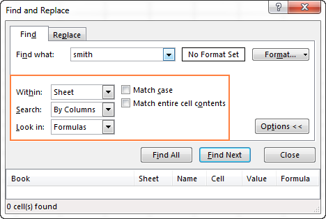
Note: In the following example, we’ve clicked the Options >> button to show the entire Find dialog. By default, it will display with Options hidden.

-
In the Find what: box, type the text or numbers you want to find, or click the arrow in the Find what: box, and then select a recent search item from the list.
Tips: You can use wildcard characters — question mark (?), asterisk (*), tilde (~) — in your search criteria.
-
Use the question mark (?) to find any single character — for example, s?t finds «sat» and «set».
-
Use the asterisk (*) to find any number of characters — for example, s*d finds «sad» and «started».
-
Use the tilde (~) followed by ?, *, or ~ to find question marks, asterisks, or other tilde characters — for example, fy91~? finds «fy91?».
-
-
Click Find All or Find Next to run your search.
Tip: When you click Find All, every occurrence of the criteria that you are searching for will be listed, and clicking a specific occurrence in the list will select its cell. You can sort the results of a Find All search by clicking a column heading.
-
Click Options>> to further define your search if needed:
-
Within: To search for data in a worksheet or in an entire workbook, select Sheet or Workbook.
-
Search: You can choose to search either By Rows (default), or By Columns.
-
Look in: To search for data with specific details, in the box, click Formulas, Values, Notes, or Comments.
Note: Formulas, Values, Notes and Comments are only available on the Find tab; only Formulas are available on the Replace tab.
-
Match case — Check this if you want to search for case-sensitive data.
-
Match entire cell contents — Check this if you want to search for cells that contain just the characters that you typed in the Find what: box.
-
-
If you want to search for text or numbers with specific formatting, click Format, and then make your selections in the Find Format dialog box.
Tip: If you want to find cells that just match a specific format, you can delete any criteria in the Find what box, and then select a specific cell format as an example. Click the arrow next to Format, click Choose Format From Cell, and then click the cell that has the formatting that you want to search for.
Replace
To replace text or numbers, press Ctrl+H, or go to Home > Editing > Find & Select > Replace.
Note: In the following example, we’ve clicked the Options >> button to show the entire Find dialog. By default, it will display with Options hidden.

-
In the Find what: box, type the text or numbers you want to find, or click the arrow in the Find what: box, and then select a recent search item from the list.
Tips: You can use wildcard characters — question mark (?), asterisk (*), tilde (~) — in your search criteria.
-
Use the question mark (?) to find any single character — for example, s?t finds «sat» and «set».
-
Use the asterisk (*) to find any number of characters — for example, s*d finds «sad» and «started».
-
Use the tilde (~) followed by ?, *, or ~ to find question marks, asterisks, or other tilde characters — for example, fy91~? finds «fy91?».
-
-
In the Replace with: box, enter the text or numbers you want to use to replace the search text.
-
Click Replace All or Replace.
Tip: When you click Replace All, every occurrence of the criteria that you are searching for will be replaced, while Replace will update one occurrence at a time.
-
Click Options>> to further define your search if needed:
-
Within: To search for data in a worksheet or in an entire workbook, select Sheet or Workbook.
-
Search: You can choose to search either By Rows (default), or By Columns.
-
Look in: To search for data with specific details, in the box, click Formulas, Values, Notes, or Comments.
Note: Formulas, Values, Notes and Comments are only available on the Find tab; only Formulas are available on the Replace tab.
-
Match case — Check this if you want to search for case-sensitive data.
-
Match entire cell contents — Check this if you want to search for cells that contain just the characters that you typed in the Find what: box.
-
-
If you want to search for text or numbers with specific formatting, click Format, and then make your selections in the Find Format dialog box.
Tip: If you want to find cells that just match a specific format, you can delete any criteria in the Find what box, and then select a specific cell format as an example. Click the arrow next to Format, click Choose Format From Cell, and then click the cell that has the formatting that you want to search for.
There are two distinct methods for finding or replacing text or numbers on the Mac. The first is to use the Find & Replace dialog. The second is to use the Search bar in the ribbon.
Find & Replace dialog
Search bar and options

-
Press Ctrl+F or go to Home > Find & Select > Find.
-
In Find what: type the text or numbers you want to find.
-
Select Find Next to run your search.
-
You can further define your search:
-
Within: To search for data in a worksheet or in an entire workbook, select Sheet or Workbook.
-
Search: You can choose to search either By Rows (default), or By Columns.
-
Look in: To search for data with specific details, in the box, click Formulas, Values, Notes, or Comments.
-
Match case — Check this if you want to search for case-sensitive data.
-
Match entire cell contents — Check this if you want to search for cells that contain just the characters that you typed in the Find what: box.
-
Tips: You can use wildcard characters — question mark (?), asterisk (*), tilde (~) — in your search criteria.
-
Use the question mark (?) to find any single character — for example, s?t finds «sat» and «set».
-
Use the asterisk (*) to find any number of characters — for example, s*d finds «sad» and «started».
-
Use the tilde (~) followed by ?, *, or ~ to find question marks, asterisks, or other tilde characters — for example, fy91~? finds «fy91?».

-
Press Ctrl+F or go to Home > Find & Select > Find.
-
In Find what: type the text or numbers you want to find.
-
Select Find All to run your search for all occurrences.

Note: The dialog box expands to show a list of all the cells that contain the search term, and the total number of cells in which it appears.
-
Select any item in the list to highlight the corresponding cell in your worksheet.
Note: You can edit the contents of the highlighted cell.

-
Press Ctrl+H or go to Home > Find & Select > Replace.
-
In Find what, type the text or numbers you want to find.
-
You can further define your search:
-
Within: To search for data in a worksheet or in an entire workbook, select Sheet or Workbook.
-
Search: You can choose to search either By Rows (default), or By Columns.
-
Match case — Check this if you want to search for case-sensitive data.
-
Match entire cell contents — Check this if you want to search for cells that contain just the characters that you typed in the Find what: box.
Tips: You can use wildcard characters — question mark (?), asterisk (*), tilde (~) — in your search criteria.
-
Use the question mark (?) to find any single character — for example, s?t finds «sat» and «set».
-
Use the asterisk (*) to find any number of characters — for example, s*d finds «sad» and «started».
-
Use the tilde (~) followed by ?, *, or ~ to find question marks, asterisks, or other tilde characters — for example, fy91~? finds «fy91?».
-
-
-
In the Replace with box, enter the text or numbers you want to use to replace the search text.
-
Select Replace or Replace All.
Tips:
-
When you select Replace All, every occurrence of the criteria that you are searching for is replaced.
-
When you select Replace, you can replace one instance at a time by selecting Next to highlight the next instance.
-
-
Select any cell to search the entire sheet or select a specific range of cells to search.
-
Press Command + F or select the magnifying glass to expand the Search bar and type the text or number you want to find in the search field.
Tips: You can use wildcard characters — question mark (?), asterisk (*), tilde (~) — in your search criteria.
-
Use the question mark (?) to find any single character — for example, s?t finds «sat» and «set».
-
Use the asterisk (*) to find any number of characters — for example, s*d finds «sad» and «started».
-
Use the tilde (~) followed by ?, *, or ~ to find question marks, asterisks, or other tilde characters — for example, fy91~? finds «fy91?».
-
-
Press return.
Notes:
-
To find the next instance of the item you are searching for, press return again or use the Find dialog box and select Find Next.
-
To specify additional search options, select the magnifying glass and select Search in Sheet or Search in Workbook. You can also select the Advanced option, which launches the Find dialog.
Tip: You can cancel a search in progress by pressing ESC.
-
Find
To find something, press Ctrl+F, or go to Home > Editing > Find & Select > Find.
Note: In the following example, we’ve clicked > Search Options to show the entire Find dialog. By default, it will display with Search Options hidden.

-
In the Find what: box, type the text or numbers you want to find.
Tips: You can use wildcard characters — question mark (?), asterisk (*), tilde (~) — in your search criteria.
-
Use the question mark (?) to find any single character — for example, s?t finds «sat» and «set».
-
Use the asterisk (*) to find any number of characters — for example, s*d finds «sad» and «started».
-
Use the tilde (~) followed by ?, *, or ~ to find question marks, asterisks, or other tilde characters — for example, fy91~? finds «fy91?».
-
-
Click Find Next or Find All to run your search.
Tip: When you click Find All, every occurrence of the criteria that you are searching for will be listed, and clicking a specific occurrence in the list will select its cell. You can sort the results of a Find All search by clicking a column heading.
-
Click > Search Options to further define your search if needed:
-
Within: To search for data within a certain selection, choose Selection. To search for data in a worksheet or in an entire workbook, select Sheet or Workbook.
-
Direction: You can choose to search either Down (default), or Up.
-
Match case — Check this if you want to search for case-sensitive data.
-
Match entire cell contents — Check this if you want to search for cells that contain just the characters that you typed in the Find what box.
-
Replace
To replace text or numbers, press Ctrl+H, or go to Home > Editing > Find & Select > Replace.
Note: In the following example, we’ve clicked > Search Options to show the entire Find dialog. By default, it will display with Search Options hidden.

-
In the Find what: box, type the text or numbers you want to find.
Tips: You can use wildcard characters — question mark (?), asterisk (*), tilde (~) — in your search criteria.
-
Use the question mark (?) to find any single character — for example, s?t finds «sat» and «set».
-
Use the asterisk (*) to find any number of characters — for example, s*d finds «sad» and «started».
-
Use the tilde (~) followed by ?, *, or ~ to find question marks, asterisks, or other tilde characters — for example, fy91~? finds «fy91?».
-
-
In the Replace with: box, enter the text or numbers you want to use to replace the search text.
-
Click Replace or Replace All.
Tip: When you click Replace All, every occurrence of the criteria that you are searching for will be replaced, while Replace will update one occurrence at a time.
-
Click > Search Options to further define your search if needed:
-
Within: To search for data within a certain selection, choose Selection. To search for data in a worksheet or in an entire workbook, select Sheet or Workbook.
-
Direction: You can choose to search either Down (default), or Up.
-
Match case — Check this if you want to search for case-sensitive data.
-
Match entire cell contents — Check this if you want to search for cells that contain just the characters that you typed in the Find what box.
-
Need more help?
You can always ask an expert in the Excel Tech Community or get support in the Answers community.
Recommended articles
Merge and unmerge cells
REPLACE, REPLACEB functions
Apply data validation to cells
To replace text or numbers, press Ctrl+H, or go to Home > Find & Select > Replace. In the Find what box, type the text or numbers you want to find. In the Replace with box, enter the text or numbers you want to use to replace the search text. Click Replace or Replace All.
Contents
- 1 How do you replace multiple values in Excel?
- 2 How do you replace multiple characters in Excel?
- 3 How do I change a cell value based on another cell value in Excel?
- 4 Is there a Replace function in Excel?
- 5 How do I replace blank value in Excel?
- 6 How do you replace in numbers?
- 7 How do I replace a character in a formula in Excel?
- 8 How do you find and replace multiple words?
- 9 What is an Xlookup in Excel?
- 10 How do you change the value of a column based on another column in Excel?
- 11 How do you fix values in Excel?
- 12 How do I return blank instead of #value?
- 13 How do you fix Find and Replace in Excel?
- 14 Can you find and replace multiple words in Excel?
- 15 Which menu shows the Find Replace option?
- 16 What is the shortcut key for finding and replacing text in a document?
- 17 How do I enable Xlookup?
- 18 Is Xlookup better than index match?
- 19 Is Xlookup new?
How do you replace multiple values in Excel?
=SUBSTITUTE(A2, “1”, “2”) – Substitutes all occurrences of “1” with “2”. Note. The SUBSTITUTE function in Excel is case-sensitive. For example, the following formula replaces all instances of the uppercase “X” with “Y” in cell A2, but it won’t replace any instances of the lowercase “x”.
How do you replace multiple characters in Excel?
1. If you want to replace “Excel” with “Word” in A1. Double-click the cell B1, copy the formula =REPLACE(A1,1,4,”Excel”) to B1, press Enter, return to “Excel table technique”; double-click B2, and copy the formula =SUBSTITUTE(A1,”Word”,”Excel”) to B2, press Enter, and return also to “Excel table technique”.
How do I change a cell value based on another cell value in Excel?
Excel formulas for conditional formatting based on cell value
- Select the cells you want to format.
- On the Home tab, in the Styles group, click Conditional formatting > New Rule…
- In the New Formatting Rule window, select Use a formula to determine which cells to format.
- Enter the formula in the corresponding box.
Is there a Replace function in Excel?
The Microsoft Excel REPLACE function replaces a sequence of characters in a string with another set of characters. The REPLACE function is a built-in function in Excel that is categorized as a String/Text Function. It can be used as a worksheet function (WS) in Excel.
How do I replace blank value in Excel?
Step 1: Select the range that you will work with. Step 2: Press the F5 key to open the Go To dialog box. Step 3: Click the Special button, and it opens the Go to Special dialog box. Step 6: Now just enter 0 or any other value that you need to replace the errors, and press Ctrl + Enter keys.
How do you replace in numbers?
To replace text or numbers, press Ctrl+H, or go to Home > Find & Select > Replace. In the Find what box, type the text or numbers you want to find. In the Replace with box, enter the text or numbers you want to use to replace the search text. Click Replace or Replace All.
How do I replace a character in a formula in Excel?
Replacing strings with SUBSTITUTE
- The syntax of the SUBSTITUTE function.
- =SUBSTITUTE(text, old_text, new_text, [instance_num])
- text is the cell that contains the string you want replaced.
- old_text is the sequence of characters that you want Excel to replace.
- new_text is what Excel will insert in its place.
How do you find and replace multiple words?
Find and replace text
- Go to Home > Replace or press Ctrl+H.
- Enter the word or phrase you want to locate in the Find box.
- Enter your new text in the Replace box.
- Select Find Next until you come to the word you want to update.
- Choose Replace. To update all instances at once, choose Replace All.
What is an Xlookup in Excel?
Use the XLOOKUP function to find things in a table or range by row.With XLOOKUP, you can look in one column for a search term, and return a result from the same row in another column, regardless of which side the return column is on.
How do you change the value of a column based on another column in Excel?
There will be times when you would want to format cell or column based on another column’s value.
How does it work?
- Select any cell in D2:D12.
- Goto conditional formatting. Click on “Manage Rules”.
- Change the range in “Applies to” box to A2:A12.
- Hit OK button.
How do you fix values in Excel?
Remove spaces that cause #VALUE!
- Select referenced cells. Find cells that your formula is referencing and select them.
- Find and replace.
- Replace spaces with nothing.
- Replace or Replace all.
- Turn on the filter.
- Set the filter.
- Select any unnamed checkboxes.
- Select blank cells, and delete.
How do I return blank instead of #value?
Click the Layout & Format tab, and then do one or more of the following: Change error display Select the For error values show check box under Format. In the box, type the value that you want to display instead of errors. To display errors as blank cells, delete any characters in the box.
How do you fix Find and Replace in Excel?
In your Excel worksheet, you have to press CTRL + H in your keyboard. You will see the dialog box of Find and Replace. Now you have to type the text in the box of Find What box. In the box of Replace with, you have to type the text which you want to replace with the original one.
Can you find and replace multiple words in Excel?
The easiest way to find and replace multiple entries in Excel is by using the SUBSTITUTE function. The formula’s logic is very simple: you write a few individual functions to replace an old value with a new one.
Go to the “Home” tab menu on the Ribbon of Microsoft Word 2007/2010/2013, at the furthest right of the group is the “Editing” options. Click the Editing item, a popup menu will appear and now you can see the “Find” and “Replace” items at the top of the box.
What is the shortcut key for finding and replacing text in a document?
Ctrl + H
If you want to find and replace text in a Word document, use the key combo Ctrl + H. That will bring up the “Find and Replace” dialog box.
How do I enable Xlookup?
- Position the cell cursor in cell E4 of the worksheet.
- Click the Lookup & Reference option on the Formulas tab followed by XLOOKUP near the bottom of the drop-down menu to open its Function Arguments dialog box.
- Click cell D4 in the worksheet to enter its cell reference into the Lookup_value argument text box.
Is Xlookup better than index match?
XLOOKUP Vs VLOOKUP Vs INDEX/MATCH
Let’s recap how XLOOKUP outperforms VLOOKUP and INDEX/MATCH: It is the simplest function, with only 3 arguments needed in most cases because the default match_mode is 0 (exact match). It’s a single function, unlike INDEX/MATCH, so it’s faster to type.
Is Xlookup new?
Fortunately, the geniuses on the Microsoft Excel team have just released XLOOKUP, a brand-new function available in Office 365* that replaces VLOOKUP. (It also replaces HLOOKUP, the lesser-used function for searching horizontally, in spreadsheet rows.)
![]()
Download Article
![]()
Download Article
This wikiHow will show you how to find and replace cell values in Microsoft Excel. The Find and Replace tool is available in all versions of Excel, including the mobile Excel app.
-
1
Open your workbook in Excel. You can open your project by clicking the File menu and selecting Open. You can also open it by right-clicking the file and selecting Open With > Excel.
- This method should work for all versions of Microsoft Excel beginning with Excel 2007.
-
2
Click the Home tab. You’ll find this in the editing menu above your document.
Advertisement
-
3
Click Find & Select. You’ll find this in the «Editing» grouping of the Home tab with the icon of a magnifying glass.
-
4
Click Replace. This is usually the first listing in the drop-down menu.
-
5
Enter the original value in the «Find what» text box field. This is the text that will be replaced.
- You can use * to find a string of characters. For example, s*d will find «sad» as well as «started.»[1]
- You can use ? to replace a single character in a search. For example, s?t will find «sat» and «set.»[2]
- You can use * to find a string of characters. For example, s*d will find «sad» as well as «started.»[1]
-
6
Enter the new value in the «Replace with» text box field. This text will replace the original text.
- You can opt to match the case, so you can change every instance of «wikihow» to «wikiHow.»
- You can chose to contain your find and replace to the current worksheet or apply it to the entire workbook.
-
7
Click Replace All or Replace. If you want to decide to replace each original value individually, choose Replace, but if you want to replace all the original values at once, choose replace all.[3]


Advertisement
-
1
Open your project in Excel. This app icon looks like a green-and-white spreadsheet icon with an «X» next to it. You can find this app on the Home screen, in the app drawer, or by searching.
- If you don’t have the Excel app, you can get it for free from the App Store (iOS) and the Google Play Store (Android).
- Tap the Open tab in Excel to find all your recent documents.
-
2
Tap the search icon
that looks like a magnifying glass. You’ll see this in the top right corner of your screen.
- A search bar will appear at the top of your document.
-
3
Tap the gear icon
. You’ll see this next to the search bar that dropped down. Search options will appear.
-
4
Tap to select Find and Replace or Find and Replace All. As you tap an option, you’ll see the search bar at the top of the screen change to fit your selection.
- Tap Find and Replace if you want to replace each original value individually.
- Tap Find and Replace All if you want to replace all the original values instantly.
-
5
Tap Done (iOS) or X (Android). You’ll see this option at the top right of the search settings.
-
6
Type your original value into the «Find» bar. This is the current value located in your document.
-
7
Type the new value into the «Replace» bar. This value will replace the current value in the document.
-
8
Tap Replace or Replace All. You’ll see this with your «find and replace» terms.


Advertisement
Ask a Question
200 characters left
Include your email address to get a message when this question is answered.
Submit
Advertisement
Thanks for submitting a tip for review!
wikiHow Video: How to Replace Values in Excel
References
About This Article
Article SummaryX
To find and replace cell values on your computer, open your worksheet in Excel and click the Home tab. Click the Find & Select button on the toolbar, and then select Replace on the menu. On the «»Find and Replace»» window, enter the text you want to find into the «»Find what»» field. You can even use wildcards for a string of text. Wildcards are special characters that replace other characters in searches, like a question mark in place of a letter or an asterisk. In the «»Replace with»» field, type your replacement text exactly how it should appear. To replace all original values at once, click the Replace All button. If you’d rather approve each replacement, click Replace instead.
To replace cell values in the mobile Excel app, open Excel and select a file to edit. Tap the search icon at the top-right corner, and then tap the gear icon next to the search bar to view your options. If you want to replace multiple instances of the same text all at once, tap Find and Replace All. If you’d rather manually approve each replacement, select Replace instead. Then, Tap Done at the top-right corner. Now, type the text you want to replace into the «»Find»» bar, and the replacement text into the «»Replace»» bar. Finally, tap Replace or ‘Replace All to replace the cell values.
Did this summary help you?
Thanks to all authors for creating a page that has been read 18,609 times.
Is this article up to date?
Содержание
- SUBSTITUTE function
- Description
- Syntax
- Example
- Examples of working with text function REPLACE in Excel
- How does the REPLACE function in Excel work?
- REPLACE function in Excel and examples of its use
- How to REPLACE a piece of text in Excel cell?
- REPLACE, REPLACEB functions
- Description
- Syntax
- Example
- SUBSTITUTE Function
- Related functions
- Summary
- Purpose
- Return value
- Arguments
- Syntax
- Usage notes
- Examples
- Related functions
- How to use Find and Replace in Excel most efficiently
- How to use Find in Excel
- Find value in a range, worksheet or workbook
- Excel Find — additional options
- Find cells with specific format in Excel
- Find cells with formulas in Excel
- How to select and highlight all found entries on a sheet
- How to use Replace in Excel
- Replace one value with another
- Replace text or number with nothing
- How to find or replace a line break in Excel
- How to change cell formatting on the sheet
- Excel Find and Replace with wildcards
- How to find and replace wildcard characters in Excel
- Shortcuts for find and replace in Excel
- Search and replace in all open workbooks
SUBSTITUTE function
This article describes the formula syntax and usage of the SUBSTITUTE function in Microsoft Excel.
Description
Substitutes new_text for old_text in a text string. Use SUBSTITUTE when you want to replace specific text in a text string; use REPLACE when you want to replace any text that occurs in a specific location in a text string.
Syntax
SUBSTITUTE(text, old_text, new_text, [instance_num])
The SUBSTITUTE function syntax has the following arguments:
Text Required. The text or the reference to a cell containing text for which you want to substitute characters.
Old_text Required. The text you want to replace.
New_text Required. The text you want to replace old_text with.
Instance_num Optional. Specifies which occurrence of old_text you want to replace with new_text. If you specify instance_num, only that instance of old_text is replaced. Otherwise, every occurrence of old_text in text is changed to new_text.
Example
Copy the example data in the following table, and paste it in cell A1 of a new Excel worksheet. For formulas to show results, select them, press F2, and then press Enter. If you need to, you can adjust the column widths to see all the data.
=SUBSTITUTE(A2, «Sales», «Cost»)
Substitutes Cost for Sales (Cost Data)
=SUBSTITUTE(A3, «1», «2», 1)
Substitutes first instance of «1» with «2» (Quarter 2, 2008)
=SUBSTITUTE(A4, «1», «2», 3)
Substitutes third instance of «1» with «2» (Quarter 1, 2012)
Источник
Examples of working with text function REPLACE in Excel
REPLACE function is included in the text functions of MS Excel and is intended to replace a specific area of the text string containing the source text on the specified text line (new text).
How does the REPLACE function in Excel work?
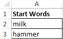
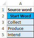
Example 1. In order to study in detail the operation of this function, we consider one of the simplest examples. Suppose we have several words in different columns, we need to get new words using the original ones. For this example, in addition to our main function REPLACE, we also use the RIGHT function — this function serves to return a certain number of characters from the end of a line of text. That is, for example, we have two words: milk and a skating rink, as a result we must get the word hammer.
REPLACE function in Excel and examples of its use
- Create a table with words on the sheet of the Excel spreadsheet workbook, as shown in the figure:
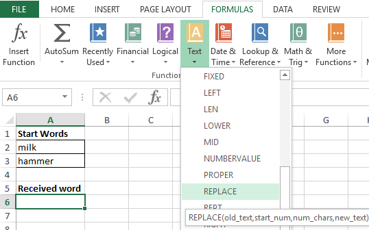
- Next, on the sheet of the workbook, we will prepare an area for placing our result — the resulting word “hammer”, as shown below. Place the cursor in cell A6 and call the function REPLACE:
- Fill the function with the arguments shown in the figure:
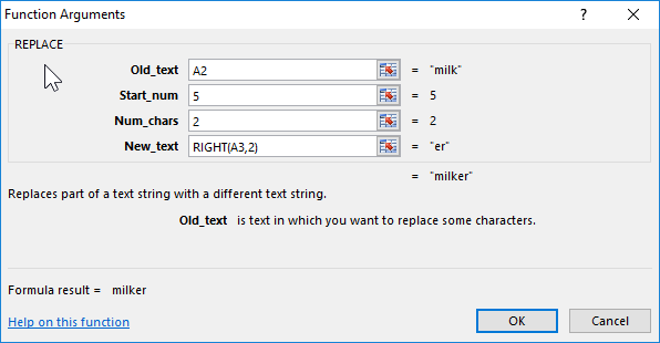
Let us explain the choice of these parameters as follows: cell A2 was chosen as the beginning of the text, the number 5 was set as beginning_, since it is from the fifth position of the word “Milk” we don’t take characters for our final word, the number_ of signs was set equal to 2, since this number It is not taken into account in the new word, as the new text, the set option RIGHT with the parameters of the cell A3 and taking the last two characters «ok».
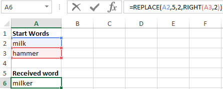
Next, click on the «OK» button and get the result:
How to REPLACE a piece of text in Excel cell?
Example 2. Consider another small example. Suppose we have columns of words in the cells of the Excel spreadsheet. It is necessary to replace their letters in certain places so as to convert them.
- Let’s create a tablet with words on the sheet of an Excel workbook, as shown in the figure:
- Further, on the same sheet of the working book we will prepare an area for placing our result — modified words. Fill the cells with two types of formulas as shown in the picture:
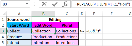
Note! In the second formula, we use the operator “&” to add the character «s» to the male surname to convert it to the female. To solve this problem, one could use the function =CONCATENATE(B3,»s») instead of the formula =B3&»s» — the result is identical. But today it is strongly recommended to abandon this formula as it has its limitations and is more demanding on resources in comparison with a simple and convenient ampersand operator.
Источник
REPLACE, REPLACEB functions
This article describes the formula syntax and usage of the REPLACE and REPLACEB function in Microsoft Excel.
Description
REPLACE replaces part of a text string, based on the number of characters you specify, with a different text string.
REPLACEB replaces part of a text string, based on the number of bytes you specify, with a different text string.
These functions may not be available in all languages.
REPLACE is intended for use with languages that use the single-byte character set (SBCS), whereas REPLACEB is intended for use with languages that use the double-byte character set (DBCS). The default language setting on your computer affects the return value in the following way:
REPLACE always counts each character, whether single-byte or double-byte, as 1, no matter what the default language setting is.
REPLACEB counts each double-byte character as 2 when you have enabled the editing of a language that supports DBCS and then set it as the default language. Otherwise, REPLACEB counts each character as 1.
The languages that support DBCS include Japanese, Chinese (Simplified), Chinese (Traditional), and Korean.
Syntax
REPLACE(old_text, start_num, num_chars, new_text)
REPLACEB(old_text, start_num, num_bytes, new_text)
The REPLACE and REPLACEB function syntax has the following arguments:
Old_text Required. Text in which you want to replace some characters.
Start_num Required. The position of the character in old_text that you want to replace with new_text.
Num_chars Required. The number of characters in old_text that you want REPLACE to replace with new_text.
Num_bytes Required. The number of bytes in old_text that you want REPLACEB to replace with new_text.
New_text Required. The text that will replace characters in old_text.
Example
Copy the example data in the following table, and paste it in cell A1 of a new Excel worksheet. For formulas to show results, select them, press F2, and then press Enter. If you need to, you can adjust the column widths to see all the data.
Источник
SUBSTITUTE Function
Summary
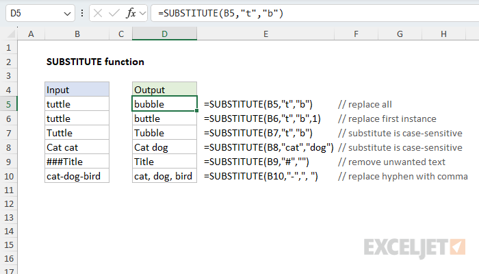
The Excel SUBSTITUTE function replaces text in a given string by matching. For example =SUBSTITUTE(«952-455-7865″,»-«,»») returns «9524557865»; the dash is stripped. SUBSTITUTE is case-sensitive and does not support wildcards.
Purpose
Return value
Arguments
- text — The text to change.
- old_text — The text to replace.
- new_text — The text to replace with.
- instance — [optional] The instance to replace. If not supplied, all instances are replaced.
Syntax
Usage notes
The Excel SUBSTITUTE function can replace text by matching. Use the SUBSTITUTE function when you want to replace text based on matching, not position. Optionally, you can specify the instance of found text to replace (i.e. first instance, second instance, etc.).
SUBSTITUTE is case-sensitive. To replace one or more characters with nothing, enter an empty string («»).
Examples
Below are the formulas used in the example shown above:
The SUBSTITUTE function cannot replace more than one string at a time. However, SUBSTITUTE can be nested inside of itself to accomplish the same thing. For example, with the text «a (dog)» in cell A1, the formula below will strip parentheses () from text:
This same approach can be used in a more complex formula to normalize telephone numbers.
Use the REPLACE function to replace text at a known location in a text string. Use the SUBSTITUTE function to replace text by searching when the location is not known. Use FIND or SEARCH to determine the location of specific text.
Источник
How to use Find and Replace in Excel most efficiently
 by Svetlana Cheusheva, updated on February 7, 2023
In this tutorial, you will learn how to use Find and Replace in Excel to search for specific data in a worksheet or workbook, and what you can do with those cells after finding them. We will also explore the advanced features of Excel search such as wildcards, finding cells with formulas or specific formatting, find and replace in all open workbooks and more.
When working with big spreadsheets in Excel, it’s crucial to be able to quickly find the information you want at any particular moment. Scanning through hundreds of rows and columns is certainly not the way to go, so let’s have a closer look at what the Excel Find and Replace functionality has to offer.
How to use Find in Excel
Below you will find an overview of the Excel Find capabilities as well as the detailed steps on how to use this feature in Microsoft Excel 365, 2021, 2019, 2016, 2013, 2010 and older versions.
Find value in a range, worksheet or workbook
The following guidelines tell you how to find specific characters, text, numbers or dates in a range of cells, worksheet or entire workbook.
- To begin with, select the range of cells to look in. To search across the entire worksheet, click any cell on the active sheet.
- Open the Excel Find and Replace dialog by pressing the Ctrl + F shortcut. Alternatively, go to the Home tab >Editing group and click Find & Select >Find…
- In the Find what box, type the characters (text or number) you are looking for and click either Find All or Find Next.


When you click Find Next, Excel selects the first occurrence of the search value on the sheet, the second click selects the second occurrence, and so on.
When you click Find All, Excel opens a list of all the occurrences, and you can click any item in the list to navigate to the corresponding cell. 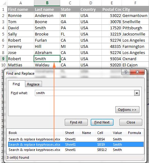
Excel Find — additional options
To fine-tune your search, click Options in the right-hand corner of the Excel Find & Replace dialog, and then do any of the following:
- To search for the specified value in the current worksheet or entire workbook, select Sheet or Workbook in the Within.
- To search from the active cell from left to right (row-by-row), select By Rows in the Search To search from top to bottom (column-by-column), select By Columns.
- To search among certain data type, select Formulas, Values, or Comments in the Look in.
- For a case-sensitive search, check the Match case check.
- To search for cells that contain only the characters you’ve entered in the Find what field, select the Match entire cell contents.
Tip. If you want to find a given value in a range, column or row, select that range, column(s) or row(s) before opening Find and Replace in Excel. For example, to limit your search to a specific column, select that column first, and then open the Find and Replace dialog.
Find cells with specific format in Excel
To find cells with certain formatting, press the Ctrl + F shortcut to open the Find and Replace dialog, click Options, then click the Format… button in the upper right corner, and define your selections in Excel Find Format dialog box. 
If you want to find cells that match a format of some other cell on your worksheet, delete any criteria in the Find what box, click the arrow next to Format, select Choose Format From Cell, and click the cell with the desired formatting. 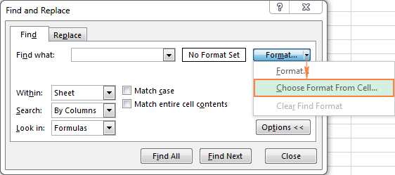
Note. Microsoft Excel saves the formatting options that you specify. If you search for some other data on a worksheet, and Excel fails to find the values that you know are there, clear the formatting options from the previous search. To do this, open the Find and Replace dialog, click the Options button on the Find tab, then click the arrow next to Format.. and select Clear Find Format.
Find cells with formulas in Excel
With Excel’s Find and Replace, you can only search in formulas for a given value, as explained in additional options of Excel Find. To find cells that contain formulas, use the Go to Special feature.
- Select the range of cells where you want to find formulas, or click any cell on the current sheet to search across the entire worksheet.
- Click the arrow next to Find & Select, and then click Go To Special. Alternatively, you can press F5 to open the Go To dialog and click the Special… button in the lower left corner.
- In the Go To Special dialog box, select Formulas, then check the boxes corresponding to the formula results you want to find, and click OK:
- Numbers — find formulas that return numeric values, including dates.
- Text — search for formulas that return text values.
- Logicals — find formulas that return Boolean values of TRUE and FALSE.
- Errors — find cells with formulas that result in errors such as #N/A, #NAME?, #REF!, #VALUE!, #DIV/0!, #NULL!, and #NUM!.


If Microsoft Excel finds any cells that meet your criteria, those cells are highlighted, otherwise a message will be displayed that no such cells have been found.
Tip. To quickly find all cells with formulas, regardless of the formula result, click Find & Select > Formulas.
How to select and highlight all found entries on a sheet
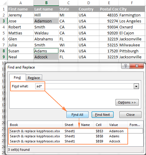
To select all occurrences of a given value on a worksheet, open the Excel Find and Replace dialog, type the search term in the Find What box and click Find All.
Excel will display a list of found entities, and you click on any occurrence in the list (or just click anywhere within the results area to move the focus there), and press the Ctrl + A shortcut. This will select all found occurrences both on the Find and Replace dialog and on the sheet. 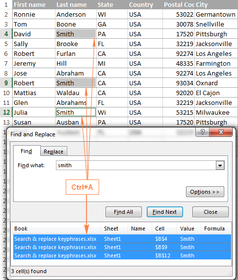
Once the cells are selected, you can highlight them by changing the fill color.
How to use Replace in Excel
Below you will find the step-by-step guidelines on how to use Excel Replace to change one value to another in a selected range of cells, entire worksheet or workbook.
Replace one value with another
To replace certain characters, text or numbers in an Excel sheet, make use of the Replace tab of the Excel Find & Replace dialog. The detailed steps follow below.
- Select the range of cells where you want to replace text or numbers. To replace character(s) across the entire worksheet, click any cell on the active sheet.
- Press the Ctrl + H shortcut to open the Replace tab of the Excel Find and Replace dialog.
Alternatively, go to the Home tab > Editing group and click Find & Select > Replace… 
If you’ve just used the Excel Find feature, then simply switch to the Replace tab.

Tip. If something has gone wrong and you got the result different from what you’d expected, click the Undo button or press Ctrl + Z to restore the original values.
For additional Excel Replace features, click the Options button in the right-hand corner of the Replace tab. They are essentially the same as the Excel Find options we discussed a moment ago.
Replace text or number with nothing
To replace all occurrences of a specific value with nothing, type the characters to search for in the Find what box, leave the Replace with box blank, and click the Replace All button. 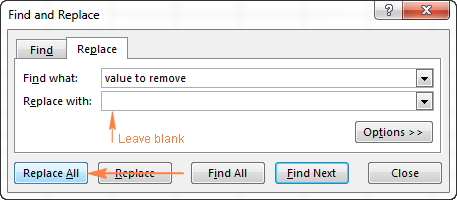
How to find or replace a line break in Excel
To replace a line break with a space or any other separator, enter the line break character in the Find what filed by pressing Ctrl + J . This shortcut is the ASCII control code for character 10 (line break, or line feed).
After pressing Ctrl + J , at first sight the Find what box will look empty, but upon a closer look you will notice a tiny flickering dot like in the screenshot below. Enter the replacement character in the Replace with box, e.g. a space character, and click Replace All. 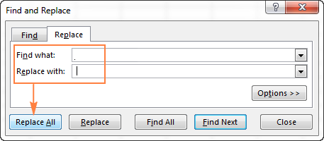
To replace some character with a line break, do the opposite — enter the current character in the Find what box, and the line break ( Ctrl + J ) in Replace with.
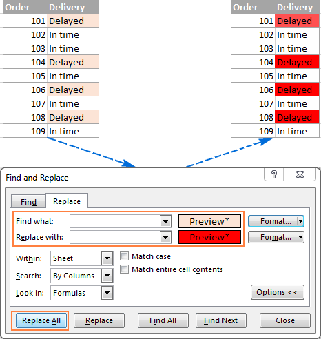
How to change cell formatting on the sheet
In the first part of this tutorial, we discussed how you can find cells with specific formatting using the Excel Find dialog. Excel Replace allows you to take a step further and change the formatting of all cells on the sheet or in the entire workbook.
- Open the Replace tab of Excel’s Find and Replace dialog, and click the Options
- Next to the Find what box, click the arrow of the Format button, select Choose Format From Cell, and click on any cell with the format you want to change.
- Next to the Replace with box, either click the Format… button and set the new format using the Excel Replace Format dialog box; or click the arrow of the Format button, select Choose Format From Cell and click on any cell with the desired format.
- If you want to replace the formatting on the entire workbook, select Workbook in the Within box. If you want to replace formatting on the active sheet only, leave the default selection (Sheet).
- Finally, click the Replace All button and verify the result.
Note. This method changes the formats applied manually, it won’t work for conditionally formatted cells.
Excel Find and Replace with wildcards
The use of wildcard characters in your search criteria can automate many find and replace tasks in Excel:
- Use the asterisk (*) to find any string of characters. For example, sm* finds «smile» and «smell«.
- Use the question mark (?) to find any single character. For instance, gr?y finds «Gray» and «Grey«.
For example, to get a list of names that begin with «ad«, use «ad*» for the search criteria. Also, please keep in mind that with the default options, Excel will search for the criteria anywhere in a cell. In our case, it would return all the cells that have «ad» in any position. To prevent this from happening, click the Options button, and check the Match entire cell contents box. This will force Excel to return only the values beginning with «ad» as shown in the below screenshot.
How to find and replace wildcard characters in Excel
If you need to find actual asterisks or question marks in your Excel worksheet, type the tilde character (
) before them. For example, to find cells that contain asterisks, you would type
* in the Find what box. To find cells that contain question marks, use
? as your search criteria.
This is how you can replace all questions marks (?) on a worksheet with another value (number 1 in this example):
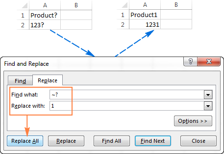
As you see, Excel successfully finds and replaces wildcards both in text and numeric values.
Tip. To find tilde characters on the sheet, type a double tilde (
) in the Find what box.
Shortcuts for find and replace in Excel
If you have been closely following the previous sections of this tutorial, you might have noticed that Excel provides 2 different ways to interact with Find and Replace commands — by clicking the ribbon buttons and by using the keyboard shortcuts.
Below there is a quick summary of what you’ve already learned and a couple more shortcuts that may save you a few more seconds.
- Ctrl+F — Excel Find shortcut that opens the Find tab of the Find & Replace
- Ctrl+H — Excel Replace shortcut that opens the Replace tab of the Find & Replace
- Ctrl+Shift+F4 — find the previous occurrence of the search value.
- Shift+F4 — find the next occurrence of the search value.
- Ctrl+J — find or replace a line break.
Search and replace in all open workbooks
As you have just see, Excel’s Find and Replace provides a lot of useful options. However, it can search only in one workbook at a time. To find and replace in all open workbooks, you can use the Advanced Find and Replace add-in by Ablebits.
The following Advanced Find and Replace features make search in Excel even more powerful:
- Find and Replace in all open workbooks or selected workbooks & worksheets.
- Simultaneous search in values, formulas, hyperlinks and comments.
- Exporting search results to a new workbook in a click.
To run the Advanced Find and Replace add-in, click on its icon on the Excel ribbon, which resides on the Ablebits Utilities tab > Search group. Alternatively, you can press Ctrl + Alt + F , or even configure it to open by the familiar Ctrl + F shortcut. 
The Advanced Find and Replace pane will open, and you do the following:
- Type the characters (text or number) to search for in the Find what
- Select in which workbooks and worksheets you want to search. By default, all sheets in all open workbooks are selected.
- Choose what data type(s) to look in: values, formulas, comments, or hyperlinks. By default, all data types are selected.
Additionally, you have the following options:
- Select the Match case option to look for case-sensitive data.
- Select the Entire cell check box to search for exact and complete match, i.e. find cells that contain only the characters you’ve typed in the Find what

Click the Find All button, and you will see a list of found entries on the Search results tab. And now, you can replace all or selected occurrences with some other value, or export the found cells, rows or columns to a new workbook. 
If you are willing to try the Advanced Find and Replace on your Excel sheets, you are welcome to download an evaluation version below.
I thank you for reading and hope to see you on our blog next week. In our text tutorial, we will dwell on Excel SEARCH and FIND as well as REPLACE and SUBSTITUTE functions, so please keep watching this space.
Источник
На чтение 1 мин
Функция ЗАМЕНИТЬ (REPLACE) в Excel используется для замены части текста одной строки, другим текстом.
Содержание
- Что возвращает функция
- Синтаксис
- Аргументы функции
- Дополнительная информация
- Примеры использования функции ЗАМЕНИТЬ в Excel
Что возвращает функция
Возвращает текстовую строку, в которой часть текста заменена на другой текст.
Синтаксис
=REPLACE(old_text, start_num, num_chars, new_text) — английская версия
=ЗАМЕНИТЬ(стар_текст;начальная_позиция;число_знаков;нов_текст) — русская версия
Аргументы функции
- old_text (стар_текст) — который вы хотите заменить;
- start_num (начальная_позиция) — стартовая позиция (порядковый номер символа), с которой вы хотите осуществить замену текста;
- num_chars (число_знаков) — количество символов, которое вы хотите заменить;
- new_text (нов_текст) — новый текст, которым вы замените текст из аргумента old_text (стар_текст).
Дополнительная информация
Аргументы стартовой позиции и количество символов для замены текста не могут быть отрицательными.
 Больше лайфхаков в нашем Telegram Подписаться
Примеры использования функции ЗАМЕНИТЬ в Excel