
Excel for Microsoft 365 for Mac Excel 2021 for Mac Excel 2019 for Mac Excel 2016 for Mac Excel for Mac 2011 More…Less
If you want to print a sheet that will have many printed pages, you can set options to print the sheet’s headings or titles on every page.
Excel automatically provides headings for columns (A, B, C) and rows (1, 2, 3). You type titles in your sheet that describe the content in rows and columns. In the following illustration, for example, Projected is a row title and 2nd QTR is a column title.
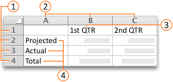
 Row headings
 Column headings
 Column titles
 Row titles
Print row and column headings
-
Click the sheet.
-
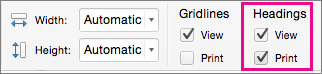
On the Page Layout tab, in the Sheet Options group, select the Print check box under Headings.

-
On the File menu, click Print.
You can see how your sheet will print in the preview pane.
Print row or column titles on every page
-
Click the sheet.
-
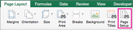
On the Page Layout tab, in the Page Setup group, click Page Setup.
-
Under Print Titles, click in Rows to repeat at top or Columns to repeat at left and select the column or row that contains the titles you want to repeat.
-
Click OK.
-
On the File menu, click Print.
You can see how your sheet will print in the preview pane.
Print row and column headings
-
Click the sheet.
-
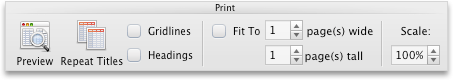
On the Layout tab, under Print, select the Headings check box.
-
On the File menu, click Print.
You can see how your sheet will print before you print it by clicking Preview.
Print row titles on every page
-
Click the sheet.
-
On the Layout tab, under Print, click Repeat Titles.
-
Click in the Columns to repeat at left box, and then on the sheet, select the column that contains the row titles.
Tip: To minimize and expand the Page Setup dialog box so that you can see more of your sheet, click
or next to the box that you clicked in. -
Click OK.
-
On the File menu, click Print.
You can see how your sheet will print before you print it by clicking Preview.
 or
or  next to the box that you clicked in.
Print column titles on every page
-
Click the sheet.
-
On the Layout tab, under Print, click Repeat Titles.
-
Under Print titles, click in the Rows to repeat at top box, and then on the sheet, select the row that contains the column titles.
Tip: To minimize and expand the Page Setup dialog box so that you can see more of your sheet, click
or next to the box that you clicked in. -
Click OK.
-
On the File menu, click Print.
You can see how your sheet will print before you print it by clicking Preview.
See also
Print part of a sheet
Print with landscape orientation
Scale the sheet size for printing
Preview pages before you print
Need more help?
Want more options?
Explore subscription benefits, browse training courses, learn how to secure your device, and more.
Communities help you ask and answer questions, give feedback, and hear from experts with rich knowledge.
Click the sheet. On the Page Layout tab, in the Page Setup group, click Page Setup. Under Print Titles, click in Rows to repeat at top or Columns to repeat at left and select the column or row that contains the titles you want to repeat. Click OK.
Contents
- 1 How do I put a header on every page in Excel?
- 2 How do you make Rows repeat in Excel when scrolling?
- 3 How do I make the first row in Excel a header?
- 4 How do you repeat a header on each page?
- 5 How do I repeat column headings at the bottom of the page in Excel?
- 6 How do I use AutoFill in Excel?
- 7 How do you repeat rows in sheets?
- 8 Where is the header row in Excel?
- 9 What is a row header?
- 10 Why is repeat header row not working?
- 11 What does repeat header rows mean?
- 12 How do you repeat a row at the bottom?
- 13 How do I repeat headers and footers in Excel?
- 14 How do I autofill an entire column in Excel?
- 15 How can I add AutoComplete to an Excel drop down validation?
- 16 How do you repeat columns in sheets?
- 17 How do you make header rows follow when scroll down worksheets?
- 18 How do I make a header row?
- 19 What is banded row in Excel?
- 20 How do I rename column names in Excel?
On the Insert tab, in the Text group, click Header & Footer. Excel displays the worksheet in Page Layout view. To add or edit a header or footer, click the left, center, or right header or footer text box at the top or the bottom of the worksheet page (under Header, or above Footer). Type the new header or footer text.
How do you make Rows repeat in Excel when scrolling?
In the worksheet which you need to repeat rows when scrolling, click View > Freeze Panes. 2. If you just want to repeat the first title row in this worksheet, please select the Freeze Top Row option from the Freeze Panes drop-down list.
With a cell in your table selected, click on the “Format as Table” option in the HOME menu. When the “Format As Table” dialog comes up, select the “My table has headers” checkbox and click the OK button. Select the first row; which should be your header row.
In the table, right-click in the row that you want to repeat, and then click Table Properties. In the Table Properties dialog box, on the Row tab, select the Repeat as header row at the top of each page check box. Select OK.
How do I repeat column headings at the bottom of the page in Excel?
MS Excel does not have a direct way of repeating rows at bottom or repeating columns at right while printing. It has options to only repeat rows or columns at top or left. One of the ways to repeat rows at the bottom of a page is to use a footer on every page.
How do I use AutoFill in Excel?
Click and hold the left mouse button, and drag the plus sign over the cells you want to fill. And the series is filled in for you automatically using the AutoFill feature. Or, say you have information in Excel that isn’t formatted the way you need it to be, such as this list of names.
How do you repeat rows in sheets?
How to Repeat the Top Row on Every Page in Google Sheets
- Open your Google Sheets file.
- Select the View tab at the top of the window.
- Click the Freeze option.
- Choose the 1 row option.
- Select File, then Print.
- Choose Headers & footers.
- Check the Repeat frozen rows option.
Row header or Row heading is the gray-colored column located on the left side of column 1 in the worksheet, which contains the numbers (1, 2, 3, etc.) where it helps out to identify each row in the worksheet.
A row heading identifies a row on a worksheet. Row headings are at the left of each row and are indicated by numbers.
Make sure that your long table is actually a single table. If it is not, then the header row won’t repeat because the table doesn’t really extend beyond a single page. The easiest way to determine if you are working with a single table vs. multiple tables is to click somewhere within the table.
Header row repetition means that the header row(s) of a table will repeat at the top of each page on which the table spans.
How do you repeat a row at the bottom?
Through the Sheet tab of the Page Setup dialog box (display the Page Layout tab of the ribbon and click the small icon at the lower-right of the Sheet Options group), Excel allows you to specify rows to repeat at the top of a printout or columns to repeat at the left of a printout.
How do I repeat headers and footers in Excel?
Click the sheet. On the Page Layout tab, in the Page Setup group, click Page Setup. Under Print Titles, click in Rows to repeat at top or Columns to repeat at left and select the column or row that contains the titles you want to repeat. Click OK.
How do I autofill an entire column in Excel?
Simply do the following:
- Select the cell with the formula and the adjacent cells you want to fill.
- Click Home > Fill, and choose either Down, Right, Up, or Left. Keyboard shortcut: You can also press Ctrl+D to fill the formula down in a column, or Ctrl+R to fill the formula to the right in a row.
How can I add AutoComplete to an Excel drop down validation?
Press Alt + Q keys simultaneously to close the Microsoft Visual Basic Applications window. From now on, when click on a drop down list cell, the drop down list will prompt automatically. You can start to type in the letter to make the corresponding item complete automatically in selected cell.
How do you repeat columns in sheets?
To repeat multiple columns N times, we can use Google Sheets REPT function. REPT is a Text function in Google Doc Spreadsheets which you can use in many ways. Here is one such example. With a custom formula using REPT, JOIN and SPLIT, we can repeat multiple columns or rows N times.
If your header row locates on the top of the worksheet, please click View > Freeze Panes > Freeze Top Rows directly. See screenshot. Now the header row is frozen. And it will follow the worksheet up and down while scrolling the worksheet.
Why create a header row in Excel?
- Organization.
- Navigation.
- Identification.
- Open Excel and the correct spreadsheet.
- Find “Page Layout” and choose “Print titles”
- Click “Rows to repeat at top” and select the header row.
- Choose a header or footer.
- Preview and print your spreadsheet.
What is banded row in Excel?
When using Excel, the term banded rows is referring to the shading of alternating rows in a worksheet. Simply put, you are applying a background color to every other row.
How do I rename column names in Excel?
Select a column, and then select Transform > Rename. You can also double-click the column header. Enter the new name.
How to Repeat Excel Spreadsheet Column Headings at Top of Page
Use this feature if you would like a title row (or rows) to print at the top of every page of your data in Excel.
Note:
If you want column headings to remain at the top of your sheet when scrolling within a spreadsheet, you will need to freeze the top row.
- Click the [Page Layout] tab > In the «Page Setup» group, click [Print Titles].
- Under the [Sheet] tab, in the «Rows to repeat at top» field, click the spreadsheet icon.
- Click and select the row you wish to appear at the top of every page.
- Press the [Enter] key, then click [OK].
- Select File > Print > «Show Print Preview» to see what the printed spreadsheet will look like.
Note:
If the [Print Titles] button is locked (greyed out), it may be because you are currently editing a cell or you have chart selected. If the «Rows to repeat at top» spreadsheet icon is locked, it may be because you have more than one worksheet selected within your workbook. To unlock either button, you can also try clicking [File] > «Print» > «Page Setup.»
Keywords: header, formatting, excel
Share This Post
-
Facebook
-
Twitter
-
LinkedIn
Examining the Data and the Issue
Our data consists of a list of apps and their monthly profit across two years of months.

If we run a Print Preview on the data, we see that the information is split across 4 pages.

The problem is that when viewing any page other than page 1, we are missing row and/or column heading information. This is especially frustrating on page 4 where we have no heading information whatsoever.

We have no idea what app or month any of the profit numbers represent.

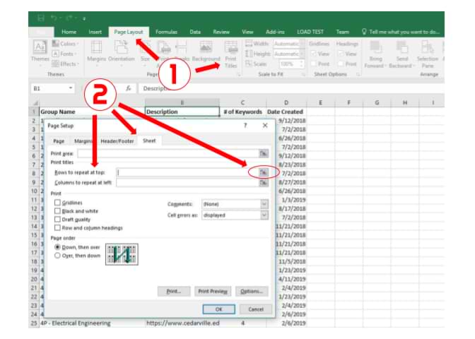
To repeat the row and/or column headings, begin by select Page Layout (tab) -> Print Setup (group) -> Print Titles.

In the Page Setup dialog box, select the Sheet tab. The controls we are interested in are in the section labeled Print Titles.

For our report, we want the list of months to be printed at the top of each page and the app names to be printed on the left of each page.
First, the month headings. In the Page Setup dialog box, click inside the field labeled “Rows to repeat at top”.
Next, click anywhere on the row containing the month headings (row 5). This will place a $5:$5 reference in the option field.

Next, the app headings. In the Page Setup dialog box, click inside the field labeled “Columns to repeat at left”.
Next, click anywhere in the column containing the app headings (column A). This will place a $A:$A reference in the option field.

Click the Print Preview button in the bottom right of the Page Setup dialog box to refresh the preview.
From any page, we remain aware of the precise app and month/year from which the profit is assigned.

One Minor Issue
If we look closely at page 3 we see the unrelated text of column A in the upper-left corner of the printout.

To keep this unrelated information from appearing, we can set out print area to only include the data we need on the printout.
Highlight the area containing the data (cells A4 through Y45) and select Page Layout (tab) -> Print Setup (group) -> Print Area -> Set Print Area.

Returning to Print Preview we can see that the unneeded text of column A has been omitted from the print result.

Keep Track of Page Order with Page Numbers
As with all multi-page printouts, especially those that traverse vertically as well as horizontally, it’s a good idea to include page numbers in either the header or footer of the pages.
The Page Layout view is one way to setup your headers and footers with page-independent information.
Two popular ways to activate the Page Layout view:
- Click the Page Layout view button (middle button) in the lower-right corner of the application window (left of the Zoom slider)

- View (tab) -> Workbook Views (group) -> Page Layout

In the Page Layout view, you can see how your report will appear when cut into individual paper-sized segments.

You also get access to the top margin that contains the header as well as the bottom margin that contains the footer.

The header and footer are broken into three segments.

Activate one of the segments by clicking inside the segment boundaries. This will activate the Header & Footer ribbon.

You can type static text directly in the segments. This is useful for things like report names, contact information, or any text that should always appear.

You can also use any of the document info “stamps” included in the Header & Footer Elements group.

Items of interest include:
- Current page number
- Total number of pages
- Print date
- Print time
- The file’s folder location
- The file’s name
- The sheet’s name
- Images (such as corporate logos)
Any of these elements can be inserted into any of the 3 header or 3 footer segments.
If we want to display the current page number along with the total number of pages, we must build this with a combination of elements and static text.
- Select a segment (ex: center of footer)
- Type the static text “Page “ (include a space after the word “page”)
- Click the Page Numbers element
- Type the static text “ of “ (include a space before and after the word “of”)
- Click the Number of Pages element


QUICK TIP: You can also insert pre-configured headers and footers by selecting the Header or Footer buttons (left side of Header & Footer button).

If you see a selection with multiple entries separated by commas, the commas indicate segment divisions.


Conclusion
As we can see, with a few clicks and a few seconds, we can transform a difficult to read report into something much more useful.
Published on: January 2, 2020
Last modified: February 27, 2023


Leila Gharani
I’m a 5x Microsoft MVP with over 15 years of experience implementing and professionals on Management Information Systems of different sizes and nature.
My background is Masters in Economics, Economist, Consultant, Oracle HFM Accounting Systems Expert, SAP BW Project Manager. My passion is teaching, experimenting and sharing. I am also addicted to learning and enjoy taking online courses on a variety of topics.
Excel now supports millions of rows. It is easy to get lost working with large datasets to figure out the meaning of the values. Repeating header rows can help us with this problem. In this tutorial, we will learn how to keep the top line visible in Excel.
Excel Repeat Header Row when Scrolling
We can repeat header rows in Excel using the Freeze Pane options. If we have one row to freeze, we can use the Freeze Top Row to modify the worksheet so the first row is always visible. In other cases where we have multiple header rows, we can use the Freeze Panes option. This helps us in Excel to always show the top row.
How to Make Column Headers Scroll in Excel Using Freeze Top Row
We use a student information database in this example. Column A, B, and C has the names, IDs and ages.
 Figure 1. The Sample Data Set
To Repeat row when scrolling, we need to:
- Click on cell A1. Drag the selection to cells A1 to A3. These are the labels we want to repeat while scrolling.
- Click on the View tab on the ribbon.
- From here, Click on the arrow next to the Freeze Panes option in the Window group.
- This will open the freezing options. We need to choose to Freeze Top Row.
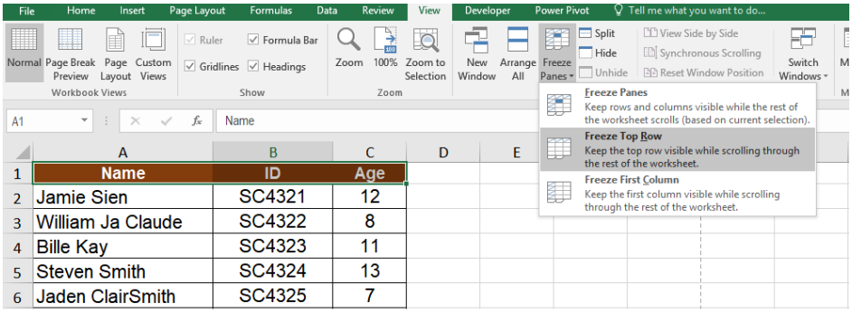 Figure 2. Example of the Freeze Pane Options
This will make the first row always visible in Excel.
 Figure 3. Repeat Header Row When Scrolling with Freeze Top Row
After we Freeze the row, the Freeze Panes option turns into Unfreeze Panes. This is a quick way to unfreeze the row.
 Figure 4. The Unfreeze Panes Option
How to Make a Column Stay in Excel Containing Multiple Header Rows
Sometimes, we may have tables having multiple header rows. These might be a bit different from the usual table structures. But, they help to understand the data clearly. We have to modify the worksheet so the first row is always visible when we scroll the worksheet down. We can achieve that using the Freeze Panes feature.
In this example, we use a student grade database. Column A and B have the details, C has the grades, column D and E contain whether the student has passed or not.
 Figure 5. Data with a Header Containing Two Rows
To freeze the header rows.
- We need to select cell A3.
- Follow steps 1 and 2 from the previous example.
- From here, we need to select the Freeze Panes option. This lets us lock several rows at once.
 Figure 6. Repeat Header Rows with the Freeze Panes Option
Notes
- It is a good habit to unfreeze the rows at first if it does not work.
- When the rows are locked in the table, we will see the Unfreeze Panes option in place of Freeze Panes. It is a good practice to look at the option name at first before attempting to lock or unlock the row.
How to Keep Title Row when Scrolling in Google Sheets
We can repeat header rows when scrolling in Google Sheets using the Freeze option. To lock the first row from the previous example:
- We need to select cells A1 to A3.
- Next, we need to click View.
- From here, we need to click Freeze > 1 Row.
 Figure 7. The Freeze Option in Google Sheets
This will repeat the header row when scrolling in Google Sheets.
 Figure 8. Example of Repeating Header Rows when Scrolling in Google Sheets
We can freeze multiple rows by selecting 2 Rows or Up to current row from the Freeze options.
 Figure 9. Example of repeating 2 rows when scrolling in Google Sheets
Repeating header rows help to work with large datasets without getting lost. The Freeze options help us to repeat header rows in both Excel and Google Sheets. This saves a lot of time and makes working with large datasets comparatively easier.
Instant Connection to an Excel Expert
Most of the time, the problem you will need to solve will be more complex than a simple application of a formula or function. If you want to save hours of research and frustration, try our live Excelchat service! Our Excel Experts are available 24/7 to answer any Excel question you may have. We guarantee a connection within 30 seconds and a customized solution within 20 minutes.