
Find and remove duplicates
Excel for Microsoft 365 Excel 2021 Excel 2019 Excel 2016 Excel 2013 Excel 2010 Excel 2007 Excel Starter 2010 More…Less
Sometimes duplicate data is useful, sometimes it just makes it harder to understand your data. Use conditional formatting to find and highlight duplicate data. That way you can review the duplicates and decide if you want to remove them.
-
Select the cells you want to check for duplicates.
Note: Excel can’t highlight duplicates in the Values area of a PivotTable report.
-
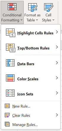
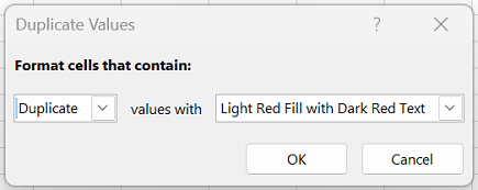
Click Home > Conditional Formatting > Highlight Cells Rules > Duplicate Values.

-
In the box next to values with, pick the formatting you want to apply to the duplicate values, and then click OK.
Remove duplicate values
When you use the Remove Duplicates feature, the duplicate data will be permanently deleted. Before you delete the duplicates, it’s a good idea to copy the original data to another worksheet so you don’t accidentally lose any information.
-
Select the range of cells that has duplicate values you want to remove.
-
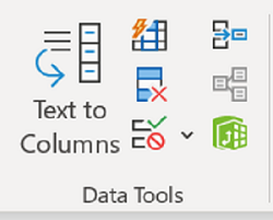
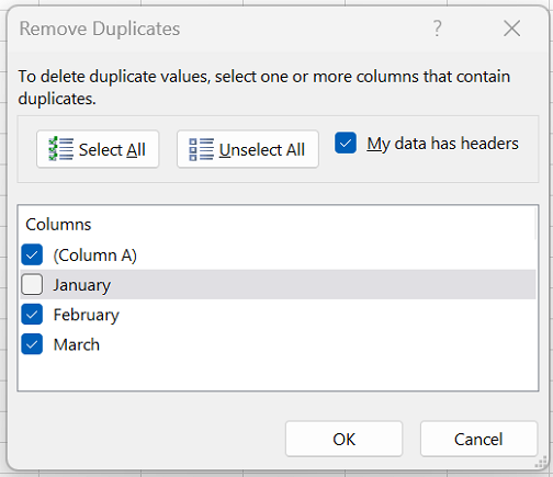
Click Data > Remove Duplicates, and then Under Columns, check or uncheck the columns where you want to remove the duplicates.
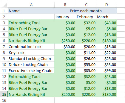
For example, in this worksheet, the January column has price information I want to keep.
So, I unchecked January in the Remove Duplicates box.
-
Click OK.
Note: The counts of duplicate and unique values given after removal may include empty cells, spaces, etc.
Need more help?

Need more help?
Содержание
- Repeat value in excel
- Table of Contents
- How to create an array formula
- Explaining array formula in cell A6
- Step 1 — Count previous values
- Step 2 — Compare array values to list
- Step 3 — Match first FALSE value in array
- Step 4 — Return a value of the cell at the intersection of a particular row and column
- Get the Excel file
- Repeat values in a predetermined series
- Repeat Cell Value N times in Excel
- 1. Repeat Cell Value N Times using VLOOKUP Function
- 2. Repeat Cell Value N Times with VBA Code
- 3. Video: Repeat Cell Value N Times in Excel
- 4. Conclusion
- REPT Function in Excel
- Excel REPT Function
- Syntax
- Examples to use REPT Function in Excel
- Example #1 – Repeat a set of characters
- Example #2 – Repeat a character
- Example #3 – Equalize the length of the numbers
- Example #4 – Create in-cell charts
- Things to Remember
- Recommended Articles
- Premium Excel Course Now Available!
- Build Professional — Unbreakable — Forms in Excel
- 45 Tutorials — 5+ Hours — Downloadable Excel Files
- REPT Function in Excel — Repeat Values
- Syntax
- Example
- Notes
- Question? Ask it in our Excel Forum
- VBA Course — Beginner to Expert
- Subscribe for Weekly Tutorials
- BONUS: subscribe now to download our Top Tutorials Ebook!
Repeat value in excel
This article explains how to repeat specific values based on a table, the table contains the items to be repeated and how many times they will be repeated.
The array formula in cell A6 utilizes the table and repeats the values until the condition is met.
There is also a section below that explains how to repeat values in sequence based on corresponding numbers.
Table of Contents
Array formula in cell A6:
How to create an array formula
- Double press with left mouse button on cell A6 so the prompt appears.
- Copy and paste the array formula above to the cell.
- Press and hold CTRL + SHIFT simultaneously.
- Press Enter once.
- Release all keys.
You can check using the formula bar that you did above steps right, Excel tells you if a cell contains an array formula by surrounding the formula with a beginning and ending curly brackets, like this: <=array_formula>.
Don’t enter these characters yourself they show up automatically if you did the above steps correctly.
Explaining array formula in cell A6
I recommend that you use the built-in «Evaluate Formula» feature in Excel to better understand and troubleshoot formulas, it is a great tool that allows you to see each calculation step.
Go to tab «Formulas» on the ribbon, then press with left mouse button on «Evaluate Formula» button. Press with left mouse button on «Evaluate» button to move to next calculation step, press with left mouse button on «Close» button to dismiss the dialog box.
Step 1 — Count previous values
The COUNTIF function counts values in a cell range based on a condition, however, in this case, I use a growing cell reference that expands when you copy the cell and paste to cells below.
This will make the COUNTIF function count based on multiple conditions, this technique is what makes you required to enter the formula as an array formula.
This way the function keeps track of previous values above the current cell so the correct number of values is returned based on the table.
The first argument is $A$5:A5 which is a cell reference, however, it contains two parts. The first part is an absolute cell reference pointing to A5, you can tell that it is absolute by the $ characters.
It means that the cell reference is locked to cell A5, both the column and row number is, locked, and does not change when you copy the cell to cells below. There are exceptions to this like inserting new rows or columns.
The second part is a relative cell reference and this changes when you copy the cell and paste to cells below which is great because the cell reference expands and takes multiple cells into account.
For example, in cell A6 the cell reference is $A$5:A5, however, in cell A7 the cell reference changes to $A$5:A6 and this makes the formula aware of previous returned values above the current cell.
In cell A6 there are no previous values above, only cell A5 which is empty.
The COUNTIF function returns an array containing the same number of values as the table and each value in the array represents how many times the values in the table have been displayed.
An array uses commas and semicolons to separate values, commas are between columns and semicolons are between rows.
Step 2 — Compare array values to list
This step checks if the values in the array is equal to the numbers in the table, this works because the values in the array correspond to the numbers in the table.
The equal sign compares the returned values from the COUNTIF function with the values in cell range B1:B4 and returns TRUE or FALSE. Note that the cell reference to B1:B4 is absolute. We don’t want it to change when the cell is copied to cells below.
Not a single value meets the criteria in the table in cell A6, that is why all values in the array are FALSE.
Step 3 — Match first FALSE value in array
The MATCH function returns the position of a given value in a cell range or array.
MATCH(lookup_value, lookup_array, [match_type])
The first argument is FALSE, we want to know the position of the first value that has not been repeated the number of times specified in the table.
The second argument is the array we created in step 2 and the third argument is 0 (zero) which means we want an exact match.
Step 4 — Return a value of the cell at the intersection of a particular row and column
The INDEX function returns a value from a cell range or array based on a row and column number. The column number is optional if the cell range is only a single column.
INDEX($A$1:$A$4, MATCH(FALSE, COUNTIF($A$5:A5, $A$1:$A$4)=$B$1:$B$4, 0))
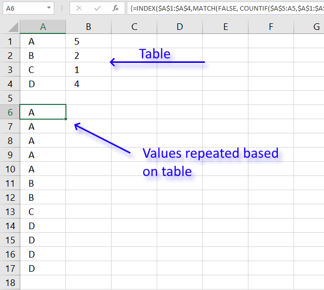
and returns A in cell A6.
Get the Excel file
Repeat values in a predetermined series
This example demonstrates a formula that repeats values in a given sequence and also how many times each value is to be repeated.
Источник
Repeat Cell Value N times in Excel
This post will guide you through two different methods to repeat cell values N times in Excel, including using the VLOOKUP function, and VBA code.
1. Repeat Cell Value N Times using VLOOKUP Function
Assuming that you have a list of data that contain two column and one column is cell value that you want to repeat, and another column contain N number. To repeat cell value N times in Excel, just do the following steps:
Step1: Insert a column to the left of A, so your current A and B columns are now B and C.
Step2: Put 1 in Cell A1.
Step3: Put =A1+C1 in A2 and drag the AutoFill Handle down to Cell A5.
Step4: Put an empty string in B5, by just entering a single quote (‘) in the cell
Step5: Put a number 1 in E1, a number 2 in E2, and copy down as to get 1, 2, …, 14
Step6: Type the following formula based on the VLOOKUP function into the formula box of cell F1 and then drag the AutoFill Handle over other cells to apply this formula.
2. Repeat Cell Value N Times with VBA Code
You can also use the VBA Code to select a range of cells, then select the destination cell and repeat N time for the selected range of cells based on the next cell in the same row. Just do the following steps:
Step1: Press ALT+F11 to open the Visual Basic Editor.
Step2: Click on Insert > Module.
Step3: Paste the following code into the module.
Step4: Press F5 to execute the code. Or press ALT+F8 to open the Macro dialog box. And select the Macro RepeatCellValuesNTimes_excelhow from the Macro list. Click Run button.
Step5: Select the range of cells that you want to repeat the value in, and click OK.
Step6: Select the destination cell where you want to start repeating the value, and click OK.
Step7: The value will be repeated N times in separate cells.
3. Video: Repeat Cell Value N Times in Excel
This video will show you how to repeat cell value N times in Excel using both the VLOOKUP formula and VBA code.
4. Conclusion
These methods have its own benefits and drawbacks, so it’s important to choose the one that best fits your needs. Through those two methods, you’ll be able to easily repeat any cell value N times in Excel.
Источник
REPT Function in Excel


Excel REPT Function
The REPT function is also known as the repeat function in Excel. As the name suggests, this function repeats the provided data according to the given number of times. So, this function takes two arguments: the first is the text that needs to be repeated, and the second is the number of times we want the text to be repeated.
For example,=REPT(“p”,3) returns “ppp.”
Table of contents
Syntax
Below is the REPT formula in Excel.

Arguments
- text= It is a required parameter. It is the text to be repeated.
- number_of_times =It is also a required parameter. It is the number of times the text in parameter-1 is to be repeated. It must be a positive number.
Examples to use REPT Function in Excel
The REPT function is a Worksheet (WS) function. Therefore, the REPT function can be inserted as a part of the formula in a worksheet cell as a WS function. Refer to a couple of examples given below to know more.
Example #1 – Repeat a set of characters
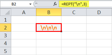
In the above example, REPT(“n,” 3) “n” is said to be repeated 3 times. As a result, cell B2 contains “nnn.”
Example #2 – Repeat a character
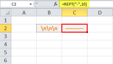
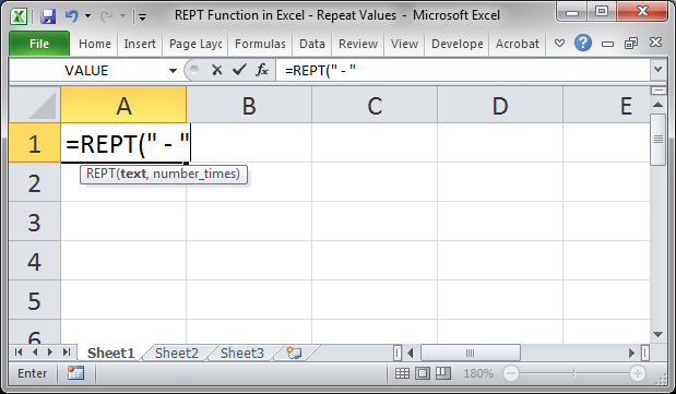
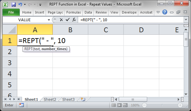
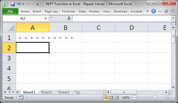
In the above example, REPT (“-,” 10) “-” is said to be repeated 10 times. As a result, cell C1 contains “———-.”
Example #3 – Equalize the length of the numbers
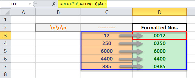
In the above example, column C contains a series of numbers from C3 to C7.
The number of digits each cell contains is different. So, the use case is to make all the numbers of the same length by adding zeros (0) so that the value of the number does not change, but all the numbers become of the same length.
Here, the length defined is 4. That is, all the numbers should be of length 4. The formatted numbers are in column D, starting from D3 to D7. So, the formatted number of C3 is present in D3, C4 in D4, C5 in D5, C6 in D6, C7 in D7, and so on. Each cell from D3 to D7 has a REPT function applied to it.
Here, the REPT function is used to add leading or trailing zeros. First, let us analyze the REPT function written in the formula bar.
As shown in the above REPT formula in Excel, “0” represents a digit/text to be repeated. The second parameter is the frequency with which zero is to be repeated. Here, the length of the number in the C3 cell is deducted from number 4, which will give us the number of zeros to be repeated to format the number in 4-digit format.
E. g: If the length of the number present in C3 is 2, then 4-2=2, which is evaluated to – REPT (“0”,2), meaning repeat 0 twice. Further, the resultant number ends with the original value, which here is 12, and the result is 0012.
Example #4 – Create in-cell charts
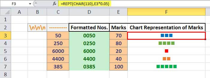
In the above example, column E contains a series of marks obtained out of 100 from E3 to E7. Therefore, it will represent the marks obtained in a graphical format without using the default charts widget in Excel. We can accomplish it by using the REPT function, as explained below.
Here, the REPT formula is =REPT(CHAR(110), E3*0.05).
All characters have an ASCII code, which is understood by the computer. For example, small case ‘n’ has code 110. So, =CHAR (110) in Excel returns ‘n.’ When “Wingdings” font is applied on the same, it becomes a block displayed as – n.
Now, we have got the character to be repeated. Now, we must figure out how many times it is to be repeated. So, the REPT function is applied to calculate the number of blocks: – E3*0.05, meaning one block would represent 1/5th of the value. So, the number of blocks for marks 70 is shown as 3 repeated blocks in the result cell F3.
A similar formula is repeated on the remaining values, from E4 to E7, resulting in 4, 1, 2, and 5 blocks for marks 80, 20, 40, and 100 shown in the result cells F4, F5, F6, F7, respectively.
Things to Remember
- The second parameter of the REPT function must be a positive number.
- If it is 0 (zero), the REPT function returns “” i.e., an empty text.
- If it is not an integer, it is truncated.
- The result of the REPT function cannot be longer than 32,767 characters. Else, the REPT formula returns #VALUE! Error indicating an error with the value.
Recommended Articles
This article is a guide to the REPT Function in Excel. Here, we discuss the REPT formula and how to use it in Excel, along with examples and a downloadable Excel template. You may also look at these useful functions in Excel: –
Источник
Premium Excel Course Now Available!
Build Professional — Unbreakable — Forms in Excel
45 Tutorials — 5+ Hours — Downloadable Excel Files
REPT Function in Excel — Repeat Values
BLACK FRIDAY SALE (65%-80% Off)
Excel Courses Online
Video Lessons Excel Guides
Quickly repeat a value, character, or number within a cell in Excel. This is a neat little function that is easy to use and can help to create some unique elements within the spreadsheet or just perform a simple character repeat.
Syntax
| Argument | Description |
|---|---|
| Text | What you want to repeat, surrounded by double quotation marks. |
| How many times you want to repeat the text. |
Example
- Type =REPT(
- Put the text or characters that you want repeated within double quotation marks.
- Type a comma and then input how many times you want to repeat it.
- Hit Enter and that’s it.

Notes
You can do this with text, numbers, characters, basically anything you can type in-between two quotation marks.
The value in the cell will still be a function, if you want to turn it into the text that you see, use this tutorial to change formulas into their output values in Excel.
Make sure to download the accompanying tutorial to see this function in the worksheet.
Question? Ask it in our Excel Forum
Excel VBA Course — From Beginner to Expert
200+ Video Lessons 50+ Hours of Instruction 200+ Excel Guides
Become a master of VBA and Macros in Excel and learn how to automate all of your tasks in Excel with this online course. (No VBA experience required.)
VBA Course — Beginner to Expert
Subscribe for Weekly Tutorials
BONUS: subscribe now to download our Top Tutorials Ebook!
The link to our top 15 tutorials has been sent to you, check your email to download it!
(If you don’t see the email, check your Spam or Promotions folder and make sure to add us as a contact so you get our emails in the future.)
Excel VBA Course — From Beginner to Expert
200+ Video Lessons
50+ Hours of Video
200+ Excel Guides
Become a master of VBA and Macros in Excel and learn how to automate all of your tasks in Excel with this online course. (No VBA experience required.)
Источник
Author: Oscar Cronquist Article last updated on January 16, 2023
This article explains how to repeat specific values based on a table, the table contains the items to be repeated and how many times they will be repeated.
The array formula in cell A6 utilizes the table and repeats the values until the condition is met.
There is also a section below that explains how to repeat values in sequence based on corresponding numbers.
BatTodor asks:
I failed to find the right article in your blog and therefore I want to ask you in newest post. So I have a table similar to this:
A 5
B 2
C 1
D 4
Is it possible with a formula to generate a list like this:
A
A
A
A
A
B
B
C
D
D
D
D
Thank you in advance!
Array formula in cell A6:
=INDEX($A$1:$A$4, MATCH(FALSE, COUNTIF($A$5:A5, $A$1:$A$4)=$B$1:$B$4, 0))
How to create an array formula
- Double press with left mouse button on cell A6 so the prompt appears.
- Copy and paste the array formula above to the cell.
- Press and hold CTRL + SHIFT simultaneously.
- Press Enter once.
- Release all keys.
You can check using the formula bar that you did above steps right, Excel tells you if a cell contains an array formula by surrounding the formula with a beginning and ending curly brackets, like this: {=array_formula}.
Don’t enter these characters yourself they show up automatically if you did the above steps correctly.
Explaining array formula in cell A6
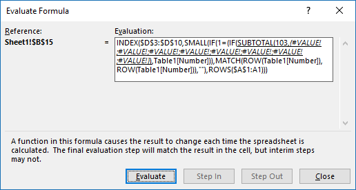
I recommend that you use the built-in «Evaluate Formula» feature in Excel to better understand and troubleshoot formulas, it is a great tool that allows you to see each calculation step.
Go to tab «Formulas» on the ribbon, then press with left mouse button on «Evaluate Formula» button. Press with left mouse button on «Evaluate» button to move to next calculation step, press with left mouse button on «Close» button to dismiss the dialog box.
Step 1 — Count previous values
The COUNTIF function counts values in a cell range based on a condition, however, in this case, I use a growing cell reference that expands when you copy the cell and paste to cells below.
This will make the COUNTIF function count based on multiple conditions, this technique is what makes you required to enter the formula as an array formula.
This way the function keeps track of previous values above the current cell so the correct number of values is returned based on the table.
COUNTIF($A$5:A5,$A$1:$A$4)
COUNTIF(range, criteria)
The first argument is $A$5:A5 which is a cell reference, however, it contains two parts. The first part is an absolute cell reference pointing to A5, you can tell that it is absolute by the $ characters.
It means that the cell reference is locked to cell A5, both the column and row number is, locked, and does not change when you copy the cell to cells below. There are exceptions to this like inserting new rows or columns.
The second part is a relative cell reference and this changes when you copy the cell and paste to cells below which is great because the cell reference expands and takes multiple cells into account.
For example, in cell A6 the cell reference is $A$5:A5, however, in cell A7 the cell reference changes to $A$5:A6 and this makes the formula aware of previous returned values above the current cell.
COUNTIF($A$5:A5,$A$1:$A$4)
becomes
COUNTIF(«»,{«A»;»B»;»C»;»D»})
and returns {0;0;0;0}
In cell A6 there are no previous values above, only cell A5 which is empty.
The COUNTIF function returns an array containing the same number of values as the table and each value in the array represents how many times the values in the table have been displayed.
An array uses commas and semicolons to separate values, commas are between columns and semicolons are between rows.
Step 2 — Compare array values to list
This step checks if the values in the array is equal to the numbers in the table, this works because the values in the array correspond to the numbers in the table.
The equal sign compares the returned values from the COUNTIF function with the values in cell range B1:B4 and returns TRUE or FALSE. Note that the cell reference to B1:B4 is absolute. We don’t want it to change when the cell is copied to cells below.
COUNTIF($A$5:A5,$A$1:$A$4)=$B$1:$B$4
becomes
{0;0;0;0}={5;2;1;4}
and returns {FALSE;FALSE;FALSE;FALSE}
Not a single value meets the criteria in the table in cell A6, that is why all values in the array are FALSE.
Step 3 — Match first FALSE value in array
The MATCH function returns the position of a given value in a cell range or array.
MATCH(lookup_value, lookup_array, [match_type])
The first argument is FALSE, we want to know the position of the first value that has not been repeated the number of times specified in the table.
The second argument is the array we created in step 2 and the third argument is 0 (zero) which means we want an exact match.
MATCH(FALSE, COUNTIF($A$5:A5,$A$1:$A$4)=$B$1:$B$4,0)
becomes
MATCH(FALSE, {FALSE;FALSE;FALSE;FALSE},0)
and returns 1.
Step 4 — Return a value of the cell at the intersection of a particular row and column
The INDEX function returns a value from a cell range or array based on a row and column number. The column number is optional if the cell range is only a single column.
INDEX($A$1:$A$4, MATCH(FALSE, COUNTIF($A$5:A5, $A$1:$A$4)=$B$1:$B$4, 0))
becomes
=INDEX($A$1:$A$4, 1)
and returns A in cell A6.
Repeat values in a predetermined series
This example demonstrates a formula that repeats values in a given sequence and also how many times each value is to be repeated.
Debraj asks:
Hi Oscar,
Great Job.. Is this possible to repeat the range according to criteria in loop.. like below.Z 5
Y 2
X 1
W 4then Z 5 Times, Y 2 Times…. but in series
Z
Y
X
W
Z
Y
W
Z
W
Z
W
ZRegards,
Deb
Array formula in cell A6:
=INDEX($A$1:$A$4, MATCH(MIN(IF(COUNTIF($A$5:A5, $A$1:$A$4)=$B$1:$B$4, «», COUNTIF($A$5:A5, $A$1:$A$4))), IF(COUNTIF($A$5:A5, $A$1:$A$4)=$B$1:$B$4, «», COUNTIF($A$5:A5, $A$1:$A$4)), 0))
Explaining formula in cell A6
Step 1 — Count previous values
COUNTIF($A$5:A5, $A$1:$A$4)=$B$1:$B$4
becomes
{0;0;0;0}=$B$1:$B$4
becomes
{0;0;0;0}={5;2;1;4}
and returns
{FALSE;FALSE;FALSE;FALSE}.
Step 2 — Replace values to be repeated with their count
IF(COUNTIF($A$5:A5, $A$1:$A$4)=$B$1:$B$4, «», COUNTIF($A$5:A5, $A$1:$A$4))
becomes
IF({FALSE; FALSE; FALSE; FALSE}, «», {0;0;0;0})
and returns
{0;0;0;0}.
Step 3 — Find smallest count number
MIN(IF(COUNTIF($A$5:A5, $A$1:$A$4)=$B$1:$B$4, «», COUNTIF($A$5:A5, $A$1:$A$4)))
becomes
MIN({0;0;0;0})
and returns 0 (zero).
Step 4 — Find relative position
MATCH(MIN(IF(COUNTIF($A$5:A5, $A$1:$A$4)=$B$1:$B$4, «», COUNTIF($A$5:A5, $A$1:$A$4))), IF(COUNTIF($A$5:A5, $A$1:$A$4)=$B$1:$B$4, «», COUNTIF($A$5:A5, $A$1:$A$4)), 0)
becomes
MATCH(0, IF(COUNTIF($A$5:A5, $A$1:$A$4)=$B$1:$B$4, «», COUNTIF($A$5:A5, $A$1:$A$4)), 0)
becomes
MATCH(0, {0;0;0;0}, 0)
and returns 1.
Step 5 — Return value based on position
INDEX($A$1:$A$4, MATCH(MIN(IF(COUNTIF($A$5:A5, $A$1:$A$4)=$B$1:$B$4, «», COUNTIF($A$5:A5, $A$1:$A$4))), IF(COUNTIF($A$5:A5, $A$1:$A$4)=$B$1:$B$4, «», COUNTIF($A$5:A5, $A$1:$A$4)), 0))
becomes
INDEX($A$1:$A$4, 1)
and returns «Z» in cell A6.
There are multiple instances that you would require to find the most repeated or maximum occurring Text or Number in your Excel worksheet.
Follow this step-by-step tutorial, to learn how to use these functions to find the most frequently occurring or repeated text or number in Excel.
Also read: Calculating Ratio, Frequency, and Percentage in Excel – Quick and Easy Guide
To count the most frequently occurring text or number in Excel: We do this by using a combination of the INDEX, MODE, and MATCH functions.
Step 1. Enter the data
- Input a relevant data set in your Excel worksheet, in which you want to find the most frequently occurring text or number. Sample data values are shown below in two different columns for checking for text and numbers individually.

Step 2. Insert Index function
- Insert a function in the output cell, by inserting the INDEX function or typing in:
=INDEX(
in the above function bar

- Now, Select all the data cell values by dragging, in which you want to analyze for most repeated values
here in our example, we are performing the operation on Data 1 column. Hence, at first, we are selecting the ‘Data 1’ column. Here, selecting A3:A13

Step 3. Insert Mode function
- After selecting the data cell values, put a comma in the function bar
- After the comma, insert MODE function by typing ,MODE( after the selection
=INDEX(A3:A13, MODE(

Step 4. Insert Match function
- Now, again insert another function in the bar by typing in MATCH(
=INDEX(A3:A13, MODE(MATCH(

Step 5. Putting Values and Final Output
- After inputting of various functions, its time to enter data values,
- Select the same data values of the same column as done in Step 2
=INDEX(A3:A13, MODE(MATCH(A3:A13
- Put a comma(,) and yet again select the same data values.
=INDEX(A3:A13, MODE(MATCH(A3:A13,A3:A13
- Now, input a comma followed by a zero (0).
- Close the bracket three times and hit Enter to apply the formula.

=INDEX(A3:A13, MODE(MATCH(A3:A13,A3:A13,0)))
Now, you will be presented with the final output for the Most Repeated Value, here in the column of ‘Data 1’

We have used the same steps to find the most repeated value in the ‘Data 2’ column for numbers.
Conclusion
That’s It! We hope you learned and enjoyed this lesson on how to find the most repeated text and numbers in your Excel worksheet, stay tuned and we’ll be back soon with another awesome Excel tutorial at QuickExcel!
This Spreadsheet tutorial explains how to repeat a value into n cells in Excel 365 in a most unpredictable way.
If you want to copy rows in an Excel table, please read my post – Excel Formula to Make Duplicates of Every Row N Times.
Coming back to our topic, we can use the SUBSTITUTE function cleverly to repeat a value into n cells in Excel 365.
Why is this required?
Sometimes we may want to print a name n times to use it as a label on packages.
For that, usually, we copy-paste the value into cells in Excel. Then print it. Using a formula may make the task easier.
Why Don’t We Use the REPT (Dedicated) Function for That?
The problem with the REPT function in Excel is it repeats the value, not into n cells! You will get the output in a single cell.
For example, the following formula in cell A1 will return the text appleappleappleappleapple in that cell which is not our desired output.
=REPT("apple",5)I want “apple” in five cells. For that, we may require to split the above result by adding a comma delimiter to it.
=SPLIT(REPT("apple,",5),",")It won’t work! Do you know why?
At the time of writing this article, unfortunately, SPLIT is not available in Excel. But you can use my SPLIT alternative formula as below.
=TRANSPOSE(
   IFERROR(
      FILTERXML(
         "<a><b>"&SUBSTITUTE(REPT("apple,",5),",","</b><b>")&"</b></a>",
         "//b"
      ),"")
)
Note:- If it returns SPILL error, empty four cells to the right-hand side of the formula applied cell.
It is not the only formula-based solution to repeat a value into n cells in Excel 365. Google it. You will see a VLOOKUP approach.
But I think using the SUBSTITUTE for this purpose is a unique and unaddressed solution in Excel 365. Let’s go to that.
Generic Excel 365 Formula:
=SUBSTITUTE(value_to_repeat," ","",SEQUENCE(1,n))Here is an Excel 365 formula example.
- In cell B3, enter “Ben,” which is the name that we want to copy n times.
- In cell C3, enter 5, which is the ‘n’ here.
- As per the above syntax, we can use the following SUBSTITUTE and SEQUENCE combination to repeat the value “Ben” into 5 (n) cells.
=SUBSTITUTE(B3," ","",SEQUENCE(1,C3))
You may ask why I have kept mum about SEQUENCE.
It’s because the SEQUENCE is not a must here as it just returns an array of sequence numbers.
You can replace that with {1,2,3,4,5}.
=SUBSTITUTE(B3," ","",{1,2,3,4,5})But we will stick with SEQUENCE for flexibility.
How to Repeat Multiple Values into N Cells in Excel 365
Assume you have a list of names in cell range B3:B8. How to repeat those multiple values into n cells in Excel 365?
Here is the catch!
If n is the same for all the names to repeat, you can use the below array formula.
=SUBSTITUTE(B3:B8," ","",SEQUENCE(1,C3))
If not, copy the following D3 formula down.
=SUBSTITUTE(B3," ","",SEQUENCE(1,C3))
Here n is different for each text.