
Repeat specific rows or columns on every printed page
Excel for Microsoft 365 Excel for Microsoft 365 for Mac Excel 2021 Excel 2021 for Mac Excel 2019 Excel 2019 for Mac Excel 2016 Excel 2016 for Mac Excel 2013 Excel 2010 Excel 2007 Excel for Mac 2011 Excel Starter 2010 More…Less
If a worksheet spans more than one printed page, you can label data by adding row and column headings that will appear on each print page. These labels are also known as print titles.
Follow these steps to add Print Titles to a worksheet:
-
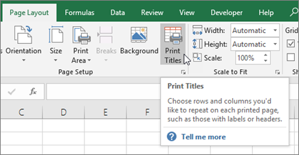
On the worksheet that you want to print, in the Page Layout tab, click Print Titles , in the Page Setup group.

Note: The Print Titles command will appear dimmed if you are in cell editing mode, if a chart is selected on the same worksheet, or if you don’t have a printer installed. For more information about installing a printer, see finding and installing printer drivers for Windows Vista. Please note that Microsoft has discontinued support for Windows XP; check your printer manufacturer’s Web site for continued driver support.
-
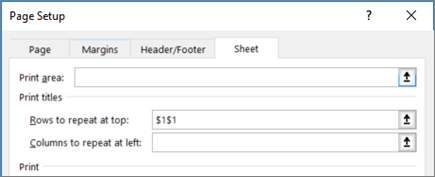
On the Sheet tab, under Print titles, do one—or both—of the following:
-
In the Rows to repeat at top box, enter the reference of the rows that contain the column labels.
-
In the Columns to repeat at left box, enter the reference of the columns that contain the row labels.
For example, if you want to print column labels at the top of every printed page, you could type $1:$1 in the Rows to repeat at top box.
Tip: You can also click the Collapse Popup Window buttons
at the right end of the Rows to repeat at top and Columns to repeat at left boxes, and then select the title rows or columns that you want to repeat in the worksheet. After you finish selecting the title rows or columns, click the Collapse Dialog button again to return to the dialog box.Note: If you have more than one worksheet selected, the Rows to repeat at top and Columns to repeat at left boxes are not available in the Page Setup dialog box. To cancel a selection of multiple worksheets, click any unselected worksheet. If no unselected sheet is visible, right-click the tab of a selected sheet, and then click Ungroup Sheets on the shortcut menu.
 at the right end of the Rows to repeat at top and Columns to repeat at left boxes, and then select the title rows or columns that you want to repeat in the worksheet. After you finish selecting the title rows or columns, click the Collapse Dialog button
 Need more help?
Click the sheet. On the Page Layout tab, in the Page Setup group, click Page Setup. Under Print Titles, click in Rows to repeat at top or Columns to repeat at left and select the column or row that contains the titles you want to repeat. Click OK.
Contents
- 1 How do I put a header on every page in Excel?
- 2 How do you make Rows repeat in Excel when scrolling?
- 3 How do I make the first row in Excel a header?
- 4 How do you repeat a header on each page?
- 5 How do I repeat column headings at the bottom of the page in Excel?
- 6 How do I use AutoFill in Excel?
- 7 How do you repeat rows in sheets?
- 8 Where is the header row in Excel?
- 9 What is a row header?
- 10 Why is repeat header row not working?
- 11 What does repeat header rows mean?
- 12 How do you repeat a row at the bottom?
- 13 How do I repeat headers and footers in Excel?
- 14 How do I autofill an entire column in Excel?
- 15 How can I add AutoComplete to an Excel drop down validation?
- 16 How do you repeat columns in sheets?
- 17 How do you make header rows follow when scroll down worksheets?
- 18 How do I make a header row?
- 19 What is banded row in Excel?
- 20 How do I rename column names in Excel?
On the Insert tab, in the Text group, click Header & Footer. Excel displays the worksheet in Page Layout view. To add or edit a header or footer, click the left, center, or right header or footer text box at the top or the bottom of the worksheet page (under Header, or above Footer). Type the new header or footer text.
How do you make Rows repeat in Excel when scrolling?
In the worksheet which you need to repeat rows when scrolling, click View > Freeze Panes. 2. If you just want to repeat the first title row in this worksheet, please select the Freeze Top Row option from the Freeze Panes drop-down list.
With a cell in your table selected, click on the “Format as Table” option in the HOME menu. When the “Format As Table” dialog comes up, select the “My table has headers” checkbox and click the OK button. Select the first row; which should be your header row.
In the table, right-click in the row that you want to repeat, and then click Table Properties. In the Table Properties dialog box, on the Row tab, select the Repeat as header row at the top of each page check box. Select OK.
How do I repeat column headings at the bottom of the page in Excel?
MS Excel does not have a direct way of repeating rows at bottom or repeating columns at right while printing. It has options to only repeat rows or columns at top or left. One of the ways to repeat rows at the bottom of a page is to use a footer on every page.
How do I use AutoFill in Excel?
Click and hold the left mouse button, and drag the plus sign over the cells you want to fill. And the series is filled in for you automatically using the AutoFill feature. Or, say you have information in Excel that isn’t formatted the way you need it to be, such as this list of names.
How do you repeat rows in sheets?
How to Repeat the Top Row on Every Page in Google Sheets
- Open your Google Sheets file.
- Select the View tab at the top of the window.
- Click the Freeze option.
- Choose the 1 row option.
- Select File, then Print.
- Choose Headers & footers.
- Check the Repeat frozen rows option.
Row header or Row heading is the gray-colored column located on the left side of column 1 in the worksheet, which contains the numbers (1, 2, 3, etc.) where it helps out to identify each row in the worksheet.
A row heading identifies a row on a worksheet. Row headings are at the left of each row and are indicated by numbers.
Make sure that your long table is actually a single table. If it is not, then the header row won’t repeat because the table doesn’t really extend beyond a single page. The easiest way to determine if you are working with a single table vs. multiple tables is to click somewhere within the table.
Header row repetition means that the header row(s) of a table will repeat at the top of each page on which the table spans.
How do you repeat a row at the bottom?
Through the Sheet tab of the Page Setup dialog box (display the Page Layout tab of the ribbon and click the small icon at the lower-right of the Sheet Options group), Excel allows you to specify rows to repeat at the top of a printout or columns to repeat at the left of a printout.
How do I repeat headers and footers in Excel?
Click the sheet. On the Page Layout tab, in the Page Setup group, click Page Setup. Under Print Titles, click in Rows to repeat at top or Columns to repeat at left and select the column or row that contains the titles you want to repeat. Click OK.
How do I autofill an entire column in Excel?
Simply do the following:
- Select the cell with the formula and the adjacent cells you want to fill.
- Click Home > Fill, and choose either Down, Right, Up, or Left. Keyboard shortcut: You can also press Ctrl+D to fill the formula down in a column, or Ctrl+R to fill the formula to the right in a row.
How can I add AutoComplete to an Excel drop down validation?
Press Alt + Q keys simultaneously to close the Microsoft Visual Basic Applications window. From now on, when click on a drop down list cell, the drop down list will prompt automatically. You can start to type in the letter to make the corresponding item complete automatically in selected cell.
How do you repeat columns in sheets?
To repeat multiple columns N times, we can use Google Sheets REPT function. REPT is a Text function in Google Doc Spreadsheets which you can use in many ways. Here is one such example. With a custom formula using REPT, JOIN and SPLIT, we can repeat multiple columns or rows N times.
If your header row locates on the top of the worksheet, please click View > Freeze Panes > Freeze Top Rows directly. See screenshot. Now the header row is frozen. And it will follow the worksheet up and down while scrolling the worksheet.
Why create a header row in Excel?
- Organization.
- Navigation.
- Identification.
- Open Excel and the correct spreadsheet.
- Find “Page Layout” and choose “Print titles”
- Click “Rows to repeat at top” and select the header row.
- Choose a header or footer.
- Preview and print your spreadsheet.
What is banded row in Excel?
When using Excel, the term banded rows is referring to the shading of alternating rows in a worksheet. Simply put, you are applying a background color to every other row.
How do I rename column names in Excel?
Select a column, and then select Transform > Rename. You can also double-click the column header. Enter the new name.
As a user, it’s easy to get lost when tracking the meaning of values. What’s more, Excel Printouts don’t have row numbers or column letters. Learning how to create a header row in excel is the ultimate solution to save you hours of work.
Usually, working with multiple pages can be confusing since they have no labels. Consequently, you are left wondering what each row represents in your spreadsheet.
In this guide, you will learn how to add an excel header row by printing or freezing header rows. So, you needn’t get lost anymore when tracking the values of multiple pages.
Creating Header Rows in Excel
Let’s dive into different methods to achieve creating header rows in Microsoft excel.
Method 1: Repeat Header Row across Multiple Spreadsheets by Printing
Assuming you want to print an excel document that spans different pages. However, on printing, you get the shock of your life that only one page has column titles. Relax. Change the settings in the Page Set-up to repeat the top header row in excel for every page.
Here’s how to repeat header row in Excel:
- First, open the Excel worksheet that needs printing.
- Navigate to the Page Layout Menu.
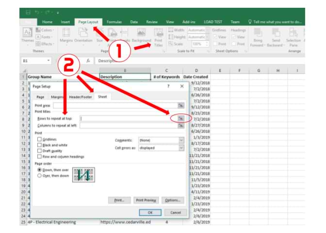
- In the Page Set-Up group, now click on Print Titles.
- The Print title command is inactive or dim if you are editing a cell. What’s more, selecting a chart in the same worksheet also dims this command.
- Alternatively, click on the Page Set-up arrow button below the Print Titles.
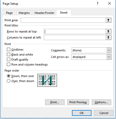
- Click on the Sheet tab from the Page Setup dialogue box.

- Under the print titles section, identify the Rows to repeat at the top section
- Ensure that you select only one workbook to repeat the headers. Otherwise, if you have several worksheets, the Rows to repeat at top and Columns to repeat at left section are invisible or greyed out.
- Click in the Rows to repeat at the top section
- Now, click on the excel header row in your spreadsheet that you want to repeat
- The Rows to repeat at top field formula is generated as shown belowAlternatively,
- Click on the Collapse Dialog icon next to the Rows to repeat at the top section.
Now, this action minimizes the page setup window, and you can resume to the worksheet. - Select the header rows that you want to repeat using the black cursor with one click
- After that, click the Collapse Dialog icon or ENTER to return to the Page Setup dialogue box.
- Click on the Collapse Dialog icon next to the Rows to repeat at the top section.
The selected rows are now displayed in the Rows to repeat at the top field, as shown below.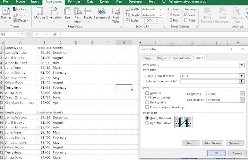
- Now, click on the Print Preview at the bottom of the Page Setup dialogue box.
- If you are happy with the results, click OK.
The header rows will be repeated on all pages of your worksheet when you print as shown in the images below.

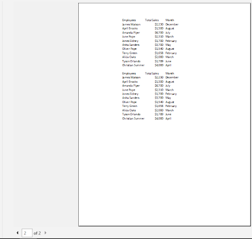
Good job! Now you are an expert on how to repeat header rows in excel.
Method 2: Freezing Excel Header Row
You can create header rows by freezing them. That way, the row headers stay in place as you scroll down the rest of the spreadsheet.
- First, open your desired spreadsheet
- Next, click the View tab and select Freeze Panes
- Click on Freeze Top from the drop-down menu
Automatically, the top row, which is the row headings, is frozen as indicated by the grey gridlines. When you scroll down or up, the header rows remain in place.
Alternatively,
- Open your excel spreadsheet
- Click on the row below your header rows
- Navigate to the View tab
- Click on Freeze Panes
- From the drop-down menu, select Freeze Panes
Excel automatically locks the header row by displaying a grey line on the gridlines. That way, your row headers remain visible in the entire spreadsheet.
Method 3: Format your Spreadsheet as a Table with Header Rows
Creating header rows reduces confusion when trying to figure out what each row represents. To format your sheet as a table with row headings, here’s what you need to do:
- First, select all the data in your spreadsheet
- Next, click on the Home Tab
- Navigate to Format as Table ribbon. Select your desired style, either light, medium, or dark.
- The Format As Table dialogue box appears
- Now, confirm whether the cells represent the right data for your table
- Make sure that you tick My table has headers checkbox
- Click OK.

You have successfully created a table that contains header rows. As a result, it is easy to handle data efficiently without getting confused or losing sight of valuable information.
How to Disable Excel Table Headers
Now that you have formatted your spreadsheet as a table with header rows, it’s possible to disable them. Here’s how:
- First, open your spreadsheet.
- Next, click on the Design tab on the toolbar.
- Uncheck Header Row box under the Table Styles Option
This process turns off the visibility of row headers on your spreadsheet.
A spreadsheet that lacks header rows is bound to create confusion. What’s more, it leaves you second-guessing values and reduces data efficiency. Nevertheless, you can create excel header rows by repeating header, freezing, or formatting as tables when handling valuable data. Click here to learn how to merge cells in excel.
How to Repeat Excel Spreadsheet Column Headings at Top of Page
Use this feature if you would like a title row (or rows) to print at the top of every page of your data in Excel.
Note:
If you want column headings to remain at the top of your sheet when scrolling within a spreadsheet, you will need to freeze the top row.
- Click the [Page Layout] tab > In the «Page Setup» group, click [Print Titles].
- Under the [Sheet] tab, in the «Rows to repeat at top» field, click the spreadsheet icon.
- Click and select the row you wish to appear at the top of every page.
- Press the [Enter] key, then click [OK].
- Select File > Print > «Show Print Preview» to see what the printed spreadsheet will look like.
Note:
If the [Print Titles] button is locked (greyed out), it may be because you are currently editing a cell or you have chart selected. If the «Rows to repeat at top» spreadsheet icon is locked, it may be because you have more than one worksheet selected within your workbook. To unlock either button, you can also try clicking [File] > «Print» > «Page Setup.»
Keywords: header, formatting, excel
Share This Post
-
Facebook
-
Twitter
-
LinkedIn
Excel now supports millions of rows. It is easy to get lost working with large datasets to figure out the meaning of the values. Repeating header rows can help us with this problem. In this tutorial, we will learn how to keep the top line visible in Excel.
Excel Repeat Header Row when Scrolling
We can repeat header rows in Excel using the Freeze Pane options. If we have one row to freeze, we can use the Freeze Top Row to modify the worksheet so the first row is always visible. In other cases where we have multiple header rows, we can use the Freeze Panes option. This helps us in Excel to always show the top row.
How to Make Column Headers Scroll in Excel Using Freeze Top Row
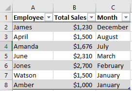
We use a student information database in this example. Column A, B, and C has the names, IDs and ages.
 Figure 1. The Sample Data Set
To Repeat row when scrolling, we need to:
- Click on cell A1. Drag the selection to cells A1 to A3. These are the labels we want to repeat while scrolling.
- Click on the View tab on the ribbon.
- From here, Click on the arrow next to the Freeze Panes option in the Window group.
- This will open the freezing options. We need to choose to Freeze Top Row.
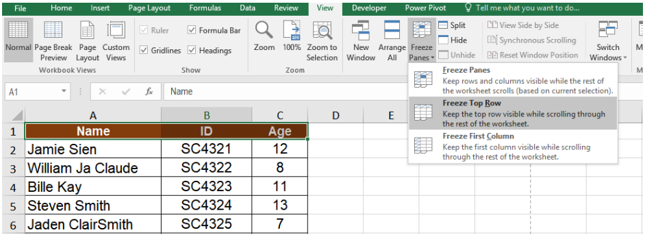 Figure 2. Example of the Freeze Pane Options
This will make the first row always visible in Excel.
 Figure 3. Repeat Header Row When Scrolling with Freeze Top Row
After we Freeze the row, the Freeze Panes option turns into Unfreeze Panes. This is a quick way to unfreeze the row.
 Figure 4. The Unfreeze Panes Option
How to Make a Column Stay in Excel Containing Multiple Header Rows
Sometimes, we may have tables having multiple header rows. These might be a bit different from the usual table structures. But, they help to understand the data clearly. We have to modify the worksheet so the first row is always visible when we scroll the worksheet down. We can achieve that using the Freeze Panes feature.
In this example, we use a student grade database. Column A and B have the details, C has the grades, column D and E contain whether the student has passed or not.
 Figure 5. Data with a Header Containing Two Rows
To freeze the header rows.
- We need to select cell A3.
- Follow steps 1 and 2 from the previous example.
- From here, we need to select the Freeze Panes option. This lets us lock several rows at once.
 Figure 6. Repeat Header Rows with the Freeze Panes Option
Notes
- It is a good habit to unfreeze the rows at first if it does not work.
- When the rows are locked in the table, we will see the Unfreeze Panes option in place of Freeze Panes. It is a good practice to look at the option name at first before attempting to lock or unlock the row.
How to Keep Title Row when Scrolling in Google Sheets
We can repeat header rows when scrolling in Google Sheets using the Freeze option. To lock the first row from the previous example:
- We need to select cells A1 to A3.
- Next, we need to click View.
- From here, we need to click Freeze > 1 Row.
 Figure 7. The Freeze Option in Google Sheets
This will repeat the header row when scrolling in Google Sheets.
 Figure 8. Example of Repeating Header Rows when Scrolling in Google Sheets
We can freeze multiple rows by selecting 2 Rows or Up to current row from the Freeze options.
 Figure 9. Example of repeating 2 rows when scrolling in Google Sheets
Repeating header rows help to work with large datasets without getting lost. The Freeze options help us to repeat header rows in both Excel and Google Sheets. This saves a lot of time and makes working with large datasets comparatively easier.
Instant Connection to an Excel Expert
Most of the time, the problem you will need to solve will be more complex than a simple application of a formula or function. If you want to save hours of research and frustration, try our live Excelchat service! Our Excel Experts are available 24/7 to answer any Excel question you may have. We guarantee a connection within 30 seconds and a customized solution within 20 minutes.